Experimental Lognormal Modeling of Harmonics Power of Switched-Mode Power Supplies

Abstract

Switched-mode power supplies (SMPSs) are an important component in many electrical systems. As a highly non-linear device, an unavoidable side-effect of SMPS operation is its high harmonics power. One of the ways to model the harmonic power consumption profile is in terms of a random process. This paper addresses random process modeling with a corresponding probability density function (PDF), auto-covariance function (ACF) and spectral coherence. The consumed harmonics power was evaluated under different load conditions and is based on experimental results of current consumption from SMPSs. The analysis shows that harmonics power may be modeled by a lognormal distribution that is time-domain uncorrelated, and that has spectral-domain correlation modeled by a Gaussian radial basis function. Extensive discussion on the modeling results is also provided. Moreover, random simulation approach based on the modeling results was proposed.

1. Introduction

The quality of electrical power supply is now a major issue worldwide, making harmonic analysis an essential element in power system planning and design. Modern electronic power equipment is a significant source of harmonic distortion that degrades the power quality. Power system harmonic modeling and analysis is hence an important prerequisite for providing high-quality operation of a power network [1,2,3]. Switched-mode power supplies (SMPSs) are dominating modern devices for AC–DC conversion in consumer electronics. In SMPSs, a control system drives analog energy switching. As a result, even when a constant DC load current is sought, the consumed current amplitude exhibits significant variability of tens of percents, as illustrated in Figure 1.

Numerous harmonics modeling techniques were proposed. For example, nonlinear frequency domain characterization approach of harmonic behavior may be applied [4]. One of these techniques is the frequency transfer matrix technique (also termed as frequency coupling matrix), in which non-linear relations are established [5]. Another is the X-parameters technique, used split into “large” and “small” components [6]. Finally, Volterra models extend a linear transfer function into nonlinear one [7]. A further modern approach is based on self-regressive nonlinear artificial neural network with exogenous input (NARX neural network) technique [8,9].

The main strength of the mentioned techniques is their repeatability of the harmonics modeling in the same conditions. Nevertheless, these techniques do not cover the statistical nature of harmonics signals. Moreover, modeling a single device can produce different results than a group of devices due to statistical variability. To overcome this limitation, the statistical harmonics analysis was proposed. In this approach, the statistical properties of harmonics behavior are analyzed, either based on the theoretical analysis of electrical circuit properties [10,11,12] or by experimental characterization. The experiment characterization may be based on parametric probabilistic modeling, such as Gaussian mixture model (GMM) [13], or non-parametric modeling, such as kernel density estimation (KDE) [14,15].

The goal of this paper is to statistically characterize current variability based on experimental measurements. The current signal is modeled by a random process that is characterized by a corresponding metrics, such as probability density function (PDF), auto-covariance function (ACF) and spectral coherence. The main contribution of the paper is modeling PDF by multivariate lognormal distribution with the appropriate ACF and spectral coherence modeling. The proposed statistical modeling provides broader signal characterization that is possibly useful in the fields of the simulation of electrical network loads [16], cyber-security [17], digital forensics [18], device identification [19], dynamic behavior investigation [20], and others.

One of the challenges of experimental harmonics signal analysis is the issue of spectral estimation. As fast Fourier transform (FFT) resolution is typically insufficient for this task, numerous methods were proposed for enhanced spectral analysis of harmonics signals. Electrical networks and power electronics systems are of particular interest. In [21,22], the applicability of Prony and min-norm harmonic retrieval methods was evaluated. Chen et al. [23] applied a Kalman filter for this task. Medina et al. [24] reviewed network-based approaches for harmonic analysis. In [25], sparse signal decomposition is used to improve FFT performance. Kabalci et al. [26] proposed harmonic analysis based on a modified artificial bee colony (MABC) algorithm. In [27], an adaptive variational mode decomposition method is used. Balouji et al. [28] applied deep learning (DL) techniques for harmonic analysis. These methods reflect the trade-off between accuracy, required signal time-length and computational complexity. Though this paper, maximum likelihood harmonics estimation [29] was applied. One of the main strengths of this method is its convenient reversibility between spectral and time-domain presentations that makes performance validation and signal modeling easier.

The rest of the paper is organized as follows. First, the essential theory is provided in Section 2. The experimental setup is presented in Section 3. Analysis of the experimental measurements is given in Section 4 followed by a discussion in Section 5. Section 6 concludes.

2. Theory

2.1. Analysis Approach

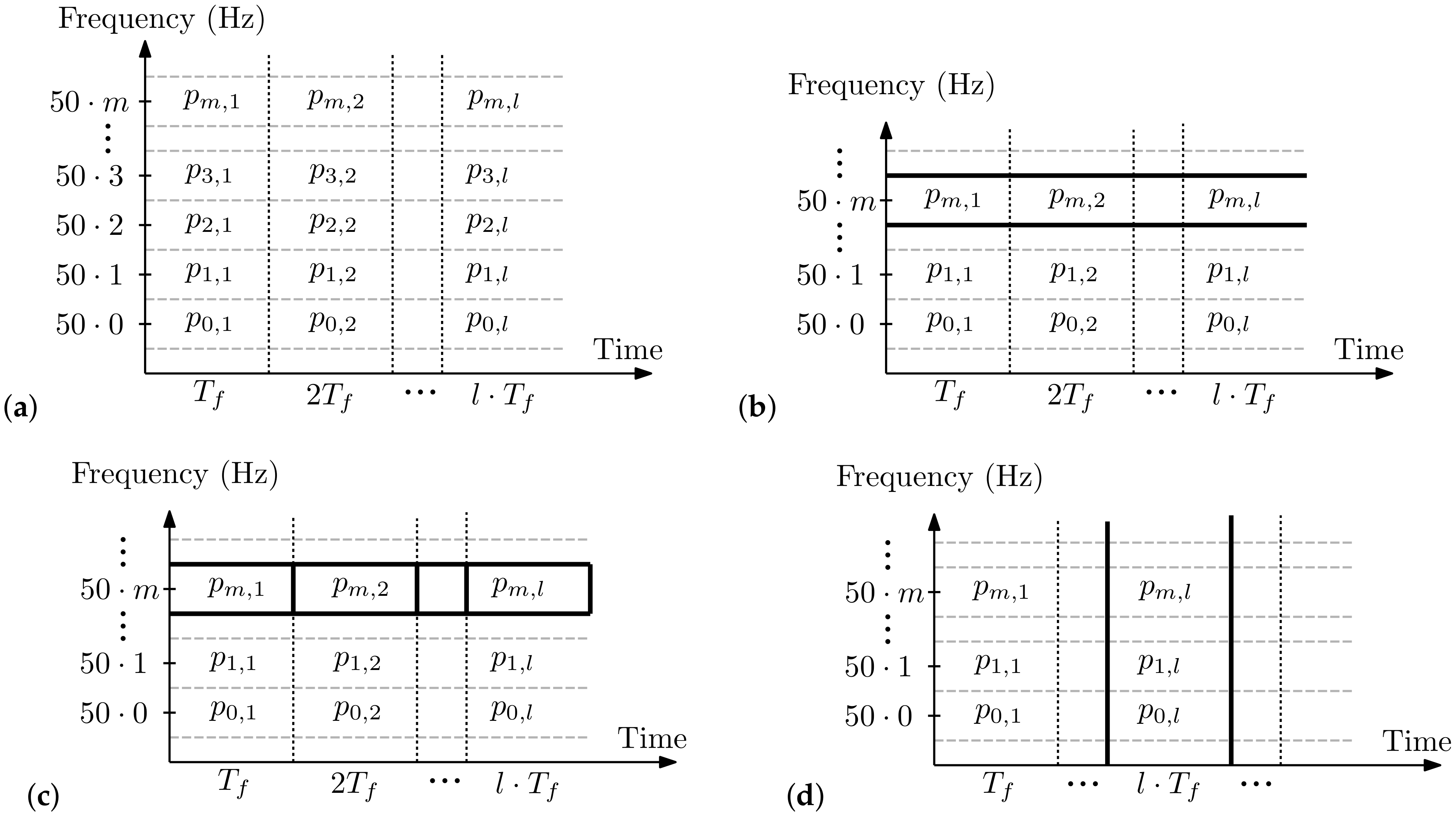
The goal of the analysis herein is to capture the changes in the harmonics signal simultaneously in both the spectral- and the time-domain. The proposed approach for this task is similar to the one applied for the short-time Fourier transform (also termed spectrogram) [30]. In this approach, the sampled signal is divided into constant-length frames of length $T_f$ with each frame independently used for harmonic analysis.

In the following, the statistical analysis approach is summarized:

• The power values of m-th harmonic at the frequency of $f_m=50·m$ [Hz] of the l-th frame, $p_{m,l}$, were evaluated by the method outlined in Section 2.2 (Figure 2a).
• The statistics of m-th harmonics power values were evaluated across all the frames as visualized in Figure 2b. The results for each harmonic were modeled by a lognormal distribution that is outlined in Section 2.3.
• The inter-harmonic relations between different frames for the same harmonics were evaluated as visualized in (Figure 2c). The evaluation was performed by an auto-covariance function (ACF), as outlined in Section 2.4.
• The analysis of intra-harmonic relations between different harmonics in the same frame were evaluated as visualized in (Figure 2c). The evaluation was based on a coherence theory outlined in Section 2.5.

2.2. Harmonics Model

In order to provide accurate spectrum estimation results, maximum likelihood harmonics estimation [29] was applied (Section 2.2.1). The most essential details on the method are provided below, and its reversibility and tractability are further discussed in Section 2.2.2.

2.2.1. Parameter Estimation

The sampled signal is divided into L frames with N samples in each frame. Each frame of a signal is modeled by the harmonics model that is formulated by a Fourier series as

$$y\left[n\right]=b_{c0}+\sum _{m=1}^M\left(b_{cm}cos\left({\omega }_{0}mn\right)+b_{sm}sin\left({\omega }_{0}mn\right)\right)+w\left[n\right],$$

(1)

where the coefficients ${\left\{b_{cm}\right\}}_{m=0}^M$ and ${\left\{b_{sm}\right\}}_{m=1}^M$ carry information on the intensity and phase of the first M harmonics of the signal, ${\omega }_0=2\pi f_0/f_s$ is the angular electrical network frequency, $f_s$ is the sampling frequency, $n=0,\dots ,N-1$ denotes time and $w\left[n\right]$ is the residual noise.

In order to simplify the presentation, Equation (1) may be rewritten as a linear relation in matrix form as

$$\mathbf{y}=\mathbf{A}\left({\omega }_0\right)\mathbf{b}+\mathbf{w},$$

(2)

where

• $\mathbf{y}$ is an $N\times 1$ vector of signal samples;
• $\mathbf{A}\left({\omega }_0\right)$ is an $N\times (2M+1)$ matrix whose n-th row is

  $$\left[1,cos\left({\omega }_{0}n\right),\dots ,cos\left({\omega }_{0}Mn\right),sin\left({\omega }_{0}n\right),\dots ,sin\left({\omega }_{0}Mn\right)\right];$$
• $\mathbf{b}$ is the corresponding coefficients vector of the form

  $$\mathbf{b}={[b_{c0},b_{c1},\dots ,b_{cM},b_{s1},\dots ,b_{sM}]}^T;$$
• $\mathbf{w}$ is the vector of noise samples.

Given the value of ${\omega }_0$, the estimation of $\mathbf{b}$ is given by a least-squares solution of the form [29]:

$$\widehat{\mathbf{b}}={\left[{\mathbf{A}}^T\left({\omega }_0\right)\mathbf{A}\left({\omega }_0\right)\right]}^{-1}{\mathbf{A}}^T\left({\omega }_0\right)\mathbf{y}.$$

(3)

The corresponding estimated power value of the m-th harmonic of the l-th frame, ${\widehat{p}}_{m,l}$, is straightforwardly found by

$${\widehat{p}}_m=\left\{\begin{array}{cc}{\widehat{b}}_{c0}^2\hfill & m=0\hfill \\ {\widehat{b}}_{cm}^2+{\widehat{a}}_{sm}^2\hfill & m\ne 0\hfill \end{array}\right.,$$

(4)

with the frame index omitted for brevity. This estimation procedure is repeated for each frame. Note, the theoretical estimation accuracy as derived by the Cramer–Rao lower bound (CRLB) under the assumption of white Gaussian noise is inverse proportional to the frame length, ∼$1/N$ [29].

In order to suppress side-lobe effects, a window of length N has to be applied on the signal $\mathbf{y}$. In this research, the Hann window [31] was chosen due to is reasonable main-lobe width and steep side-band attenuation.

2.2.2. Estimation Accuracy Evaluation

The estimated signal $\widehat{\mathbf{y}}$ may be reconstructed from the harmonics coefficients by the relation

$$\widehat{\mathbf{y}}=\mathbf{A}\left({\omega }_0\right)\widehat{\mathbf{b}},$$

(5)

and the estimated residual error signal is given by

$$\widehat{\mathbf{e}}=\mathbf{y}-\widehat{\mathbf{y}},$$

(6)

with the resulting SNR defined as the ratio of signal power divided by the residual signal power,

$$\mathrm{SNR}=\frac{{〈\widehat{\mathbf{y}}〉}^2}{{〈\widehat{\mathbf{e}}〉}^2},$$

(7)

which can be seen to be a measure of the estimation and/or reconstruction accuracy.

2.3. Lognormal Distribution

A lognormal distribution is often applied to model various natural phenomena, such as the fading behavior of radio-frequency (RF) and optical channels [32,33]. In the context of this paper, we apply the decibel-based parametrization following the convention in ([32], Chapter 2). In this convention, a lognormal distribution is defined as the Gaussian distribution of decibel values of interest ($x_{dB}=20{log}_{10}\left(x\right)$ for amplitude, $x_{dB}=10{log}_{10}\left(x\right)$ for power), with the probability density function (PDF)

$$p\left(x_{dB}\right)=\frac{1}{{\sigma }_{dB}\sqrt{2\pi }}exp(-\frac{{\left[x_{dB}-{\mu }_{dB}\right]}^2}{2{\sigma }_{dB}^2}),$$

(8)

where ${\mu }_{dB}$ and ${\sigma }_{dB}^2$ are the mean and variance of $x_{dB}$, respectively. The multivariate lognormal distribution is the extension of the univariate distribution with a covariance matrix $\Sigma$. In this paper, a lognormal distribution is applied for modeling the distribution of the m-th harmonics frequency slice (Figure 2).

2.4. Auto-Covariance Function (ACF)

The goal of the ACF is to quantify the linear dependency between time-domain samples. The normalized ACF, $C_x\left[k\right]$, is defined as the correlation coefficient between two samples of a random signal separated by k samples. In the context of this paper, the normalized ACF was applied to identify the statistical linear dependency of the same harmonic m between k-spaced frames. The ACF of the m-th harmonic was evaluated by [34]

$$C_{x_m}\left[k\right]=\frac{{\sum }_l\left(p_{m,l+k}-{\overline{p}}_m\right)\left(p_{m,l}-{\overline{p}}_m\right)}{{\sum }_l{\left(p_{m,l}-{\overline{p}}_m\right)}^2},$$

(9)

where

$${\overline{p}}_m=\frac{1}{L}\sum _l{p}_{m,l}$$

(10)

stands for power averaging of the m-th harmonic frequency slice over all frames.

2.5. Spectral Coherence

The spectral coherence describes the linear correlation coefficient between frequency components of a signal. In the context of this paper, this principle was extended to statistically characterize the correlation coefficient between different harmonics in the same time frame. The coherence between two frames $m_1$ and $m_2$ for lth harmonic was evaluated as a correlation coefficient between L-dimensional measurement vectors, $p_{m_1,l}$ and $p_{m_2,l}$, with $l=1,\dots ,L$ [35]:

$$R[m_1,m_2]=\frac{{\sum }_l\left(p_{m_1,l}-{\overline{p}}_{m_1}\right)\left(p_{m_1,2}-{\overline{p}}_{m_2}\right)}{{\sum }_l{\left(p_{m_1,l}-{\overline{p}}_{m_1}\right)}^2{\sum }_l{\left(p_{m_2,l}-{\overline{p}}_{m_2}\right)}^2},$$

(11)

where ${\overline{p}}_m$ is defined in Equation (10). When all correlation coefficients are of interest, they may be organized in a covariance matrix of size $M\times M$.

3. Experiment

3.1. Electrical Setup

The electrical setup is presented in Figure 3. The SMPS to be tested was connected to an electrical network with the consumed current measured by an ammeter (NI 9277), sampled, and logged for further off-line analysis. The DC Load (Array 3710) provides a different load current for the SMPS.

During the experiments three power supplies were evaluated:

• HP 0950-4082 with a nominal voltage of 32 V and maximum current of 940 mA;
• DVE DSA-40CA-19 with a nominal voltage of 19 V and maximum current of 1.58 A;
• SAKAL SAW012120100 with a nominal voltage of 12 V and maximum current of 1 A.

In the following, only the results for the first SMPS are presented. The results for the two other SMPSs are quite similar and are presented in the Supplementary Materials.

3.2. Analysis Configuration

Each power supply was analyzed for 10 different levels of load current ranging between unloaded level and approximate maximal current level; these levels were controlled by the DC Load. Sampling was performed at a 50 kHz frequency with 24-bit resolution. Sampling frequency was arbitrarily set to the maximum value provided by the applied equipment, as higher frequency results in higher accuracy, as outlined above in Section 2.2. Sufficient sampling resolution is required to overcome the high dynamic range difference between 50 Hz and higher frequency harmonics. The applied sampling resolution was provided by the used equipment. The frame length was set to the single 20 ms period of a 50 Hz signal, that is, 1000 samples. The applied value was set to conveniently evaluate the inter-period statistics.

4. Experimental Results

4.1. Distribution Modeling

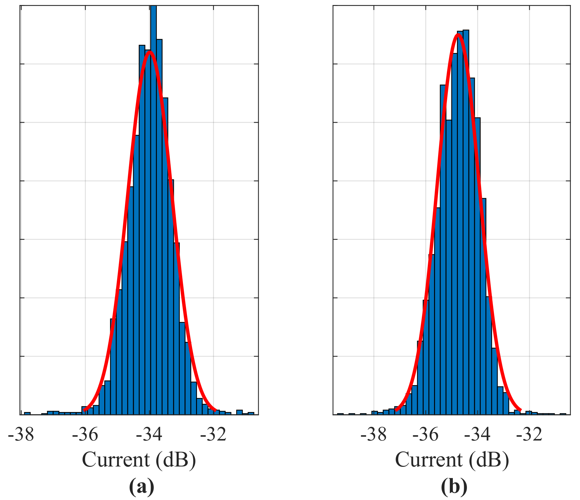
The goal of this section is to validate the lognormal distribution assumption (Section 2.3). The validation is based on the goodness-of-fit principle when the empirical PDF is compared with the theoretical one. A histogram method is used as an empirical density estimator. An example of a histogram with a Gaussian distribution fit is presented in Figure 4 and illustrates the resemblance between the empirical results and the theory.

In order to demonstrate the relations between the empirical results and the theory for different harmonics and different DC load levels, a collection of histogram fits for three different load levels and four different harmonics is presented in Figure 5. Again, the results show a significant resemblance between the empirical histograms result and the theoretic PDF of lognormal distribution for all the presented harmonics and load levels.

The characterization parameters of the lognormal distribution are ${\mu }_{dB}$ and ${\sigma }_{dB}$ that are related to the average harmonics power and the power variability. An analysis of ${\mu }_{dB}$ and ${\sigma }_{dB}$ values as a function of frequency for different load levels is presented in Figure 6. As expected, for higher frequencies, the average harmonics power is lower and the variability is higher.

The further load-dependence of the harmonics powers on the DC load current is presented by a box-plot in Figure 7. While following the results in the Figure 6 above, the results show that lower-frequency harmonics power tends to be significantly influenced by DC load current. In contrast, higher-frequency harmonics show significantly lesser consistent dependence on DC load current.

4.2. ACF Modeling

The goal of ACF evaluation is to quantify the linear statistical inter-frame relation between harmonics as defined in Section 2.4 above. The numerical evaluation of the ACF was performed as defined in Equation (9). The presented results (Figure 8) are for three different harmonics frequencies $f_m=50·m$ [Hz] with $m=1,3,5$. Three different current load levels (300 mA, 500 mA, and 700 mA) are presented.

It is common to use ACF level of 0.5 as a borderline limit between linearly dependent and independent conditions [32]. Through the evaluation, for all of the measurements, the ACF level is below 0.5. Moreover, this result holds even for consecutive frames. Therefore, the harmonics powers may be modeled, as an approximation, to be linearly independent (also termed as uncorrelated) between different frames.

4.3. Coherence Modeling

The correlation of intra-frame harmonics coefficients (Section 2.5) is visualized in Figure 9. The covariance matrices are presented in Figure 9a and show that three to five of the closest spaced harmonics are highly correlated with a significant drop-out for higher frequency spacing. An illustration of a coherence function is presented in Figure 9b, where the y-axis values are correlation coefficients as a function of a harmonics frequency. The results show significant linear statistical dependence between closely-spaced harmonics inside the same frame.

Following the presented experimental results, the proposed modeling of the coherence function (Equation (11)) is based on the Gaussian radial basic function (RBF) of the form [36]

$$R[m_1,m_2]\approx exp\left[-\frac{{\parallel m_1-m_2\parallel }^2}{b}\right].$$

(12)

This approximated modeling is suitable for a sufficiently small difference between harmonics, $\parallel m_1-m_2\parallel \lesssim 15$. The scale parameter b has to be evaluated from the measurements. An illustration of the proposed approximation is presented in Figure 9b. The corresponding b values for the presented plots are ≈83 for 50 Hz harmonic and ≈92 for 600 Hz harmonic.

5. Discussion

5.1. Estimation Accuracy

The harmonics estimation accuracy was evaluated by a comparison between the signal $\widehat{\mathbf{y}}$ (Equation (5)) reconstructed from the harmonics coefficients and the original experimental signal $\mathbf{y}$. An example of such a comparison is presented in Figure 10 for a $M=100$ harmonics and shows significant resemblance between the signals. The corresponding accuracy was quantified by SNR (Equation (7)) that measures 41.4 dB for the presented signals.

During the harmonics power evaluation, all of the resulting values were quantified by SNR. The majority of the estimated SNR values were between 39 dB and 44 dB, with a few outliers. Such values may be considered as a high outcome for an estimation procedure. Moreover, this result also shows negligible influence of inter-harmonics modulation.

5.2. Simulation

Following the assumption of time-domain independence (Section 4.2), the covariance matrix approximation (Section 4.3) and the reconstruction accuracy presented in the previous section, the harmonics signal may be modeled and simulated by a multivariate lognormal distribution. The corresponding lognormal distribution parameters (Section 2.3) are means of the distribution that are presented in Figure 6a, the values of the diagonal of the covariance matrix are presented in Figure 6b and the remaining values may be evaluated by Equation (12).

5.3. Limitations—High Load

An important applicability limitation aspect of this approach is shown for the particular modeling of even harmonics at high current load close to the upper limit current of the SMPS. For instance, see the example (Figure 11) of even harmonics for a 900 mA (out of maximum 940 mA) DC load current, where the proposed modeling is less accurate.

6. Summary and Conclusions

The main goal of this study was to model the harmonics power of a SMPS by a stationary random process using experimental data. The modeling includes stationary characterization by PDF and time-domain and frequency domain harmonics relations characterization by ACF and coherence function. The main conclusion points are:

• The lognormal distribution modeling may be applied for characterization and simulation of SMPS harmonics current consumption.
• The time-domain harmonics relation may be assumed as linearly independent.
• The frequency domain modeling may be incorporated by applying the corresponding covariance for multivariate lognormal distribution.
• The proposed method offers a new approach for random simulation the current consumption of SMPSs based on statistical harmonics modeling.

The most important limitation of this study is the number of the experimentally characterized devices. Further work is required to examine, characterize, and model the transient changes in consumed current for deferent DC load levels.

References

- Kalair, A.; Abas, N.; Kalair, A.; Saleem, Z.; Khan, N. Review of harmonic analysis, modeling and mitigation techniques. Renew. Sustain. Energy Rev. 2017, 78, 1152–1187. [Google Scholar] [CrossRef]
- Sinvula, R.; Abo-Al-Ez, K.M.; Kahn, M.T. Harmonic Source Detection Methods: A Systematic Literature Review. IEEE Access 2019, 7, 74283–74299. [Google Scholar] [CrossRef]
- Yanchenko, S.; Costa, F.B.; Strunz, K. A Simulation Tool for Accurate and Fast Assessment of Harmonic Propagation in Modern Residential Grids. IEEE Trans. Power Deliv. 2021, 36, 2118–2128. [Google Scholar] [CrossRef]
- Faifer, M.; Laurano, C.; Ottoboni, R.; Toscani, S.; Zanoni, M. Frequency-Domain Nonlinear Modeling Approaches for Power Systems Components—A Comparison. Energies 2020, 13, 2609. [Google Scholar] [CrossRef]
- Caicedo, J.; Romero, A.; Zini, H. Frequency domain modeling of nonlinear loads, considering harmonic interaction. In Proceedings of the 2017 IEEE Workshop on Power Electronics and Power Quality Applications (PEPQA), Bogota, Colombia, 31 May–2 June 2017; pp. 1–6. [Google Scholar]
- Uhl, R.; Mirz, M.; Vandeplas, T.; Barford, L.; Monti, A. Non-linear behavioral X-Parameters model of single-phase rectifier in the frequency domain. In Proceedings of the IECON 2016-42nd Annual Conference of the IEEE Industrial Electronics Society, Florence, Italy, 23–26 October 2016; pp. 6292–6297. [Google Scholar]
- Faifer, M.; Laurano, C.; Ottoboni, R.; Toscani, S.; Zanoni, M.; Crotti, G.; Giordano, D.; Barbieri, L.; Gondola, M.; Mazza, P. Overcoming Frequency Response Measurements of Voltage Transformers: An Approach Based on Quasi-Sinusoidal Volterra Models. IEEE Trans. Instrum. Meas. 2019, 68, 2800–2807. [Google Scholar] [CrossRef]
- Hatata, A.; Eladawy, M. Prediction of the true harmonic current contribution of nonlinear loads using NARX neural network. Alex. Eng. J. 2018, 57, 1509–1518. [Google Scholar] [CrossRef]
- Jumilla-Corral, A.A.; Perez-Tello, C.; Campbell-Ramírez, H.E.; Medrano-Hurtado, Z.Y.; Mayorga-Ortiz, P.; Avitia, R.L. Modeling of Harmonic Current in Electrical Grids with Photovoltaic Power Integration Using a Nonlinear Autoregressive with External Input Neural Networks. Energies 2021, 14, 4015. [Google Scholar] [CrossRef]
- Staats, P.; Grady, W.; Arapostathis, A.; Thallam, R. A statistical analysis of the effect of electric vehicle battery charging on distribution system harmonic voltages. IEEE Trans. Power Deliv. 1998, 13, 640–646. [Google Scholar] [CrossRef]
- Baghzouz, Y.; Burch, R.; Capasso, A.; Cavallini, A.; Emanuel, A.; Halpin, M.; Imece, A.; Ludbrook, A.; Montanari, G.; Olejniczak, K.; et al. Time-varying harmonics. I. Characterizing measured data. IEEE Trans. Power Deliv. 1998, 13, 938–944. [Google Scholar] [CrossRef]
- Silva, M.M.; Gonzalez, M.L.; Uturbey, W.; Carrano, E.G.; Silva, S.R. Evaluating harmonic voltage distortion in load-variating unbalanced networks using Monte Carlo simulations. IET Gener. Transm. Distrib. 2015, 9, 855–865. [Google Scholar] [CrossRef]
- Tang, Z.; Shu, Q.; Xu, F.; Jiang, Y. Novelty method for the utility harmonic impedance estimation based on Gaussian mixed model. IET Gener. Transm. Distrib. 2020, 14, 2573–2580. [Google Scholar] [CrossRef]
- Nasrfard-Jahromi, F.; Mohammadi, M. Probabilistic harmonic load flow using an improved kernel density estimator. Int. J. Electr. Power Energy Syst. 2016, 78, 292–298. [Google Scholar] [CrossRef]
- Jarkovoi, M.; Kutt, L.; Iqbal, M.N. Probabilistic bivariate modeling of harmonic current. In Proceedings of the 2020 19th International Conference on Harmonics and Quality of Power (ICHQP), Dubai, United Arab Emirates, 6–7 July 2020. [Google Scholar] [CrossRef]
- Moradi, A.; Yaghoobi, J.; Alduraibi, A.; Zare, F.; Kumar, D.; Sharma, R. Modelling and prediction of current harmonics generated by power converters in distribution networks. IET Gener. Transm. Distrib. 2021, 15, 2191–2202. [Google Scholar] [CrossRef]
- Guri, M.; Zadov, B.; Bykhovsky, D.; Elovici, Y. PowerHammer: Exfiltrating Data From Air-Gapped Computers Through Power Lines. IEEE Trans. Inf. Forensics Secur. 2020, 15, 1879–1890. [Google Scholar] [CrossRef]
- Bykhovsky, D. Recording device identification by ENF harmonics power analysis. Forensic Sci. Int. 2020, 307, 110100. [Google Scholar] [CrossRef] [PubMed]
- Ghosh, S.; Chatterjee, A.; Chatterjee, D. Improved non-intrusive identification technique of electrical appliances for a smart residential system. IET Gener. Transm. Distrib. 2019, 13, 695–702. [Google Scholar] [CrossRef]
- Zhang, J.; Ji, X.; Chi, Y.; Chen, Y.c.; Wang, B.; Xu, W. OutletSpy: Cross-outlet application inference via power factor correction signal. In Proceedings of the 14th ACM Conference on Security and Privacy in Wireless and Mobile Networks, Abu Dhabi, United Arab Emirates, 28 June–2 July 2021; pp. 181–191. [Google Scholar]
- Leonowicz, Z.; Lobos, T.; Rezmer, J. Advanced spectrum estimation methods for signal analysis in power electronics. IEEE Trans. Ind. Electron. 2003, 50, 514–519. [Google Scholar] [CrossRef]
- Lobos, T.; Leonowicz, Z.; Rezmer, J.; Schegner, P. High-Resolution Spectrum-Estimation Methods for Signal Analysis in Power Systems. IEEE Trans. Instrum. Meas. 2006, 55, 219–225. [Google Scholar] [CrossRef] [Green Version]
- Chen, C.; Chang, G.; Hong, R.; Li, H. Extended Real Model of Kalman Filter for Time-Varying Harmonics Estimation. IEEE Trans. Power Deliv. 2010, 25, 17–26. [Google Scholar] [CrossRef]
- Medina, A.; Segundo-Ramirez, J.; Ribeiro, P.; Xu, W.; Lian, K.; Chang, G.; Dinavahi, V.; Watson, N. Harmonic analysis in frequency and time domain. IEEE Trans. Power Deliv. 2013, 28, 1813–1821. [Google Scholar] [CrossRef]
- Chen, L.; Zheng, D.; Chen, S.; Han, B. Method Based on Sparse Signal Decomposition for Harmonic and Inter-harmonic Analysis of Power System. J. Electr. Eng. Technol. 2017, 12, 559–568. [Google Scholar] [CrossRef] [Green Version]
- Kabalci, Y.; Kockanat, S.; Kabalci, E. A modified ABC algorithm approach for power system harmonic estimation problems. Electr. Power Syst. Res. 2018, 154, 160–173. [Google Scholar] [CrossRef]
- Cai, G.; Wang, L.; Yang, D.; Sun, Z.; Wang, B. Harmonic Detection for Power Grids Using Adaptive Variational Mode Decomposition. Energies 2019, 12, 232. [Google Scholar] [CrossRef] [Green Version]
- Balouji, E.; Backstrom, K.; McKelvey, T.; Salor, O. Deep-Learning-Based Harmonics and Interharmonics Predetection Designed for Compensating Significantly Time-Varying EAF Currents. IEEE Trans. Ind. Appl. 2020, 56, 3250–3260. [Google Scholar] [CrossRef]
- Kay, S. Fundamentals of Statistical Signal Processing, Volume I: Estimation Theory; Prentice Hall: Hoboken, NJ, USA, 1993. [Google Scholar]
- Allen, J. Short term spectral analysis, synthesis, and modification by discrete Fourier transform. IEEE Trans. Acoust. Speech Signal Process. 1977, 25, 235–238. [Google Scholar] [CrossRef]
- Blackman, R.B.; Tukey, J.W. The measurement of power spectra from the point of view of communications engineering—Part I. Bell Syst. Tech. J. 1958, 37, 185–282. [Google Scholar] [CrossRef]
- Goldsmith, A. Wireless Communications; Cambridge University Press: Cambridge, UK, 2005. [Google Scholar]
- Bykhovsky, D. Free-space optical channel simulator for weak-turbulence conditions. Appl. Opt. 2015, 54, 9055–9059. [Google Scholar] [CrossRef] [PubMed]
- Kay, S. Intuitive Probability and Random Processes Using MATLAB; Springer: Berlin/Heidelberg, Germany, 2005. [Google Scholar]
- Gardner, W.A. A unifying view of coherence in signal processing. Signal Process. 1992, 29, 113–140. [Google Scholar] [CrossRef]
- Karimi, N.; Kazem, S.; Ahmadian, D.; Adibi, H.; Ballestra, L. On a generalized Gaussian radial basis function: Analysis and applications. Eng. Anal. Bound. Elem. 2020, 112, 46–57. [Google Scholar] [CrossRef]
Figure 1.
Illustration of a random SMPS current for a constant load.
Figure 2.
The analysis of a harmonics signal is based on the spectrogram concept, with power of l-th frame and m-th harmonic: (a) harmonics value for each time-frame; (b) statistics of m-th harmonic for all frames; (c) inter-harmonics relation; (d) intra-harmonics relation.
Figure 3.
Schematic presentation of the experimental setup.
Figure 4.
An example of the fluctuations of harmonics power (Equation (4)) at 800 mA load modeled by a lognormal distribution; the distribution is in dB units fitted with the Gaussian PDF for (a) 750 Hz harmonic and (b) 850Hz harmonic.
Figure 5.
Histogram fits of lognormal distribution for different harmonics and different DC load levels.
Figure 6.
Lognormal distribution parameters as a function of frequency for different load levels: (a) and (b) .
Figure 7.
Box-plot of the levels of the different harmonics power as a function of DC load current.
Figure 8.
ACF of harmonics power for different frequencies.
Figure 9.
Correlation of harmonics coefficients. (a) Covariance matrix visualization. (b) Selected harmonics with Gaussian radial function fit.
Figure 10.
An example of the reconstructed signal compared to the original signal.
Figure 11.
Even harmonics at high load sometimes cannot be lognormal modeled. An example of 900 mA load: (a) 100 Hz harmonic; (b)150 Hz harmonic.
Publisher’s Note: MDPI stays neutral with regard to jurisdictional claims in published maps and institutional affiliations. |
© 2022 by the author. Licensee MDPI, Basel, Switzerland. This article is an open access article distributed under the terms and conditions of the Creative Commons Attribution (CC BY) license (https://creativecommons.org/licenses/by/4.0/).
Share and Cite
MDPI and ACS Style
Bykhovsky, D. Experimental Lognormal Modeling of Harmonics Power of Switched-Mode Power Supplies. Energies 2022, 15, 653. https://doi.org/10.3390/en15020653
AMA Style
Bykhovsky D. Experimental Lognormal Modeling of Harmonics Power of Switched-Mode Power Supplies. Energies. 2022; 15(2):653. https://doi.org/10.3390/en15020653
Chicago/Turabian StyleBykhovsky, Dima. 2022. "Experimental Lognormal Modeling of Harmonics Power of Switched-Mode Power Supplies" Energies 15, no. 2: 653. https://doi.org/10.3390/en15020653
Note that from the first issue of 2016, this journal uses article numbers instead of page numbers. See further details here.