Article

Analysis of Air Pollution around a CHP Plant: Real Measurements vs. Computer Simulations

by
Robert Cichowicz
* and
Maciej Dobrzański
Faculty of Civil Engineering, Architecture and Environmental Engineering, Lodz University of Technology, Al. Politechniki 6, 90-924 Lodz, Poland
*
Author to whom correspondence should be addressed.
Energies 2022, 15(2), 553; https://doi.org/10.3390/en15020553
Submission received: 25 November 2021 / Revised: 6 January 2022 / Accepted: 10 January 2022 / Published: 13 January 2022

Abstract

:
This study examines the concentrations of air pollution in the vicinity of a combined heat and power plant (CHP) and a communication route, using computer modeling of pollutant dispersion and spatial analysis based on real measurements in the city of Łódź, Poland, Europe. The research takes into account the concentrations of particulate matter (PM10, PM2.5, PM1.0) and gaseous pollutants (SO2 and VOC) in winter and summer. The spatial distribution of pollutants is discussed, including the presence of areas with increased accumulations of pollutants. Because atmospheric air has no natural boundaries, when analyzing any location, not only local sources of pollution, but also background pollution, should be analyzed. A clear difference was observed between the concentrations of pollutants in the summer and winter seasons, with significantly higher concentrations in the winter (heating) period. The impacts of road transport, individual heating systems, and combined heat and power plants were also assessed. Computer calculations confirmed that road transport accounted for the largest share of both PM and SO2 emissions. The CHP plant was responsible for the smallest percentage of dust emissions and was the next largest producer of SO2 emissions. The share of the total emissions from the individual sources were compared with the results of detailed field tests. The numerical analysis of selected pollution sources in combination with the field analysis shows that the identified pollution sources included in the analysis represent only a part of the total observed pollutant concentrations (suggesting that other background sources account for the rest).

Graphical Abstract

1. Introduction

According to data from the European Commission’s Joint Research Center (JRS) [1], as much as 75% of the world’s population lives in urban agglomerations. In Europe, the urbanization rate was 72% in 2015 [1]. Therefore, the state of air quality in large urban agglomerations is a matter of key concern. According to a European Environment Agency (EEA) report from 2020 [2], the most frequently analyzed pollutants are PM10, PM2.5, and SO2. This is because large populations are exposed to these pollutants at concentrations higher than recommended by the EU and WHO. According to an EEA report [2], as much as 48% of the population living in urban agglomerations is exposed to concentrations of PM10 above the acceptable level of 20 µg/m3 (average annual concentration) set by the WHO in 2005 [3], and 15% of the urban population in Europe is exposed to concentrations of PM10 above the EU standard of 40 µg/m3 (average annual concentration of PM10) [4]. Moreover, 74% of the urban population is exposed to average annual concentrations of PM2.5 above the permissible level of 10 µg/m3 established by the WHO, and 19% of people are exposed to an average daily concentration of SO2 above the recommended limit of 20 µg/m3. Using less restrictive EU standards, only 4% of the European population is exposed to levels of PM2.5 beyond the permissible concentration of 25 µg/m3 and less than 1% of the European population is exposed to SO2 at levels above the recommended limit of 125 µg/m3 (24-h limit). However, in 2021, the WHO [5] updated its statements regarding permissible levels of pollutants. For PM10 and PM2.5, the permissible annual average concentrations were reduced by 25% and 50%, respectively, to 15 µg/m3 and 5 µg/m3. In the case of SO2, the permissible level was increased by 100% from 20 µg/m3 to 40 µg/m3 (average daily SO2 concentration), but this is still well below the limit permitted by the EU.
The main emitters of pollutants are the energy industry [6,7], agriculture, individual heating systems [8], and road transport [9,10]. According to the EEA [2], 41% of PM10 emissions are produced by secondary energy consumers (the commercial and public sectors, as well as private households), 10% by road transport, and 3% by the energy industry. The energy industry is responsible for as much as 47% of the emissions of gaseous pollutants, including SO2. Other industries are responsible for 33% of gaseous pollutants, while households together with the service sector and trade sector contribute 15%. This information is based on statistical data collected by air quality monitoring systems situated in all European Union member states and varies between nations. The monitoring system consists of stationary ground stations that measure pollutant concentrations in a manual daily system and an automatic continuous system [11]. Due to the low density of air quality monitoring stations, the data they collect cannot be used for a detailed analysis of the impact of individual pollution sources on local air quality. For example, in Poland there are about 0.00062 stations/km2 (in 2017, the number of PM10 measurement stations was 194). In Europe overall, the figure is about 0.00060 stations/km2 (there were 2551 PM10 measurement stations in 2017) [12]. For this reason, air quality tests carried out with mobile measurement devices [13] or using numerical programs for calculating/simulating pollutant dispersion in a selected local area are very important. Mobile measuring equipment, such as unmanned aerial vehicles, can be used to transport measuring devices [14,15] or small stationary devices [16]. Numerical programs available include Aero 2010, Emitor, OPA03 [17], AERMOD [18], ENVI-met, and Austal 2000 [19,20].
In this study, we analyzed various anthropogenic sources of pollutants in a selected area, using numerical calculations and real measurements.

2. Methodology

2.1. Analyzed Area

The analysis was focused on an urban area in the city of Łódź. Łódź is the third largest city in Poland (central-eastern Europe) in terms of the number of inhabitants (population density: 2292.2 people/km2, population: 672,185, area: 293.2 km2). The area comprises a thoroughfare running from the west to the east along Pojezierska Street, on the intersection between Aleja Włókniarzy and Zgierska Street (Figure 1).
Figure 2 shows the selected fragment of the street (no. 1) is about 1.5 km long and runs through areas of different types and purposes. We distinguish between shopping areas with large-area stores (no. 2), green areas and parks (no. 3), single-family housing areas (no. 4), multi-family developments (no. 5) and industrial areas (no. 6). The gross development index in the area ranges from 0.5 to 1.0. The analyzed street plays an important role as a road transport route connecting two main streets in the city in the east–west system. It is both a local access route to residential and industrial areas and a transit route through the city. According to [21], the average traffic volume on this road section for every 15 min is between 500 and 750 vehicles (between 2000 and 3000 vehicles per hour). In the close vicinity, there is one of the two main heat and power plants in the city, called EC-3 (Figure 2). The EC-3 combustion installation includes 9 boilers: five coal-fired steam boilers, one steam boiler fired with light fuel oil, and three water boilers fired with heavy oil. The total thermal capacity is 804 MW, and the electrical capacity is 205.85 MW [22].

2.2. Methodology of Analysis

We used both actual measurements and numerical calculations of the dispersion of emissions from selected pollution sources. Based on analysis of the research area, three probable sources of air pollution were selected: EC3 heat and power plants fired with hard coal, light, and heavy fuel oil; road transport, and individual heating systems. The actual measurements were performed in the first quarter of the year, in the period from January to March 2021 (this is the winter heating season in central and eastern Europe), and in the third quarter of the year, from June to August 2021 (the summer period in Poland). Mobile measuring equipment was used, consisting of measuring and sampling devices installed on an unmanned aerial vehicle (UAV) and on a transport platform (TP). The use of the UAV allowed for measurements at heights from 5 m to 50 m above the ground. The TP was used for measurements at a height of about 2 m above the ground. The measuring apparatus was equipped with a laser-scattered (LS) sensor, which was used to measure PM10, PM2.5, and PM1.0 (10,000 particles per second). It was also equipped with ElectroChemical (EC) sensors to measure H2S (3 ppb–1 ppm), O2 (0.20–100%), VOCs (Ethanol, Iso-Butane, 0–500 ppm, sensor type: MOS) and SO2 (0.5–2000 ppm). Validation of the measurement data of particulate matter was performed on the basis of data from an accredited measuring station VIEP (the method equivalent to the reference method), while the gaseous pollutants were validated in relation to the VEGA-GC microchromatograph (equipped with a thermal conductivity detector TCD, minimum concentration of 500 ppb (0.005 ppm)). Numerical analyses of pollutant dispersion were carried out using the ArcGis [23] program, which was used to produce a graphical presentation of the actual measurement data, and the OPA03 program by Eko-Soft [24], which was used to simulate the concentrations of pollutants from selected pollution sources. Interpolation in ArcGis was carried out using the Empirical Bayesian Kriging 3D method. Both software programs are described in detail in [14,25]. The calculations performed in the OPA03 program are based on the legal acts in force in Poland [26] and the European Union [4]. The OPA03 software is based on the proprietary algorithm of the EKO-Soft company, in accordance with the methodology described in the Polish law [26]. Data on the wind rose in the analyzed period, emitter parameters (such as the number of chimneys and their height, speed of exhaust gases, mass concentration of pollutants emitted, average hourly number of vehicles, and type of fuel) were added to the program. Details for individual pollutant emitters are presented further in the article.
The input data for the calculation of pollutant emissions from the EC-3 CHP plant were provided for scientific purposes by Veolia Energia Łódź and are the actual measurements of emissions from the CHP plant taken during the analyzed period. According to annual data, the maximum recorded emissions of PM10, PM2.5, and SO2 were 2.667 kg/h, 1.143 kg/h, and 128.81 kg/h, respectively. In accordance with the methodology presented in [27], the average volume of traffic measured during field measurements was adopted for the analysis. Different vehicle types and fuels were considered. According to [28], gasoline-powered passenger cars account for 55% of all vehicles using the analyzed communication artery, diesel-powered cars accounted for 30%, and LPG gas-powered cars for 15%. Vans were divided between those with diesel engines (75%) and those with gasoline engines (25%). Tractors and buses were 100% diesel, and 100% of motorcycles had gasoline engines (detailed data on pollutant emissions are provided later in this paper). Finally, we considered individual heating systems in single-family houses located in the immediate and close vicinity of the studied area. Individual heating systems are used for domestic hot water in summer and for heating in winter. It was assumed in the calculations that 70% of the buildings used hard coal as fuels, and 30% used natural gas.
In the numerical analysis in the OPA03 software, the simulation can be performed with or without the background level of pollution in the air. The background level of pollutions is understood as the concentration of pollutants in the air without the analyzed pollutant emitter. Background levels of pollution were not included in the numerical analyses, to illustrate the individual impact of pollution sources on the dispersion of air pollutants. A common level of 2 m above ground level was adopted for the analysis. Particulate matter pollutants PM10, PM2.5, and PM1.0 were included in the field measurements, as well as gaseous SO2 and VOCs. For the purposes of comparison, the numerical analysis was based on PM10 and SO2 emissions.

2.3. Meteorological Conditions

Characteristic data for the winter (1st quarter of the year) and summer (3rd quarter of the year) periods in central Poland were selected for the analysis. The winter period was from January to March, which is the so-called the heating period because the outside air temperatures oscillate predominantly around 0 °C. For this reason, it was decided to choose two representative measurement series, A and B, for which the average air temperature was about 6 °C with a relative humidity of about 76% (Table 1). In the summer period, from June to August, average air temperatures above 18 °C predominate. Therefore, it was decided to choose two series, C and D, in which the average temperature was higher than 20 °C.
In the analysis of the dispersion of pollutants, another important parameter is the speed and direction of the wind. In the city of Łódź in 2021, winds from the west W (11%) and west–north WSW, and SW (9%) directions were prevailing, with wind speeds ranging from 0 m/s to 7.5 m/s (Figure 3). In the winter period from January to March, the average wind speed was 2.92 m/s (11% W). In the summer period from June to August, the average wind speed was 15% lower, amounting to 2.47 m/s (9% WSW).

3. Results

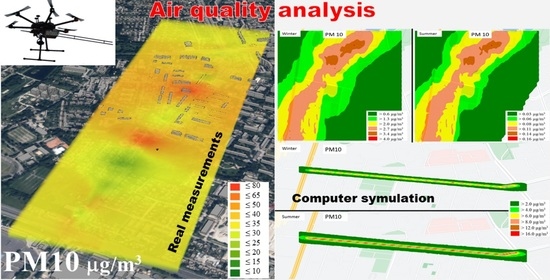
Based on the results of the field measurements, 3D maps were drawn using ArcGis software of the dispersion of pollution in the analyzed area. This form of 3D spatial analysis is an innovative approach, so the results are not comparable with the literature data. Due to the fact that dust pollution has similar field dispersion characteristics [14], PM10 pollution was selected for the graphic presentation. Figure 4 shows the results of PM10 dispersion for series A and B in the winter period, together with a longitudinal and vertical cross-section for series B to show changes in the altitude of the pollution.
The selected series of representative measurements for the winter period show a variable concentration of PM10. In series A, the average concentration of PM10 was 21.80 µg/m3 and the maximum concentration was 42.40 µg/m3. According to the air quality index adopted in Poland [30], the air quality of series A is classed as “Good” (limit of PM10 20.1–50.0 µg/m3). The spatial analysis shows that the entire area of analysis was characterized by an even concentration of PM10. In comparison, series B showed double the concentrations of PM pollutants. The mean concentration of PM10 was 54.80 µg/m3 and the maximum 77.60 µg/m3. According to the air quality index in relation to PM10, the air quality of series B is “Moderate” (50.1–80.0 µg/m3). In series A, the concentration of PM10 did not exceed the level of 50 µg/m3 allowed by EU standards, whereas in series B the EU limit was exceeded in many places by 55%. The increased concentration of particulate matter in series B can be explained by the fact that the average wind speed was less than half that in the series A. Tall buildings, with heights of 15–30 m, also contributed to the accumulation of pollution in the analyzed area. In series B, there are spaces with lower and higher PM10 concentrations. Elevated levels of PM10 > 60 µg/m3 (red in Figure 4) occur at street crossings and in more densely built-up areas. Lower PM10 concentrations (green in Figure 4) relative to the mean value occur in the highest part of the analyzed area. This is probably related to the stronger ventilation. From the vertical cross-section view of the 3D dispersion, it can be concluded that concentrations above 40 µg/m3 occur mainly close to the ground surface. At the intersections, the concentration of PM10 increases with height, which is probably related to the upward movement of pollutants and car exhaust fumes.
The concentrations of PM10 in series C and D in the summer period (Figure 5) were up to four times lower compared to the winter period. The mean concentrations of PM10 in series C and D were 8.20 µg/m3 and 12.10 µg/m3, respectively. In contrast to the winter period, during the summer period the concentration of PM10 was similar in the whole analyzed area. There were no areas with concentrations of particulate matter above the average value. Only in series D, during a period of high temperatures and low humidity, were PM10 concentrations observed exceeding 30 µg/m3, as can be seen in the upper left area of Figure 5. The source was earthworks at a construction site. To sum up, during the summer period the permissible level PM10 of 50 µg/m3 was not exceeded [4]. In the summer, the use of fuel for heating purposes in individual heating systems is reduced and the average speed of road transport increases. This contributes to lower emissions of particulate matter. To facilitate comparison of the 3D dispersion maps, further analysis of the air quality parameters was limited to two of the selected representative measurement series in order to facilitate the graphical reception and comparison of the results.
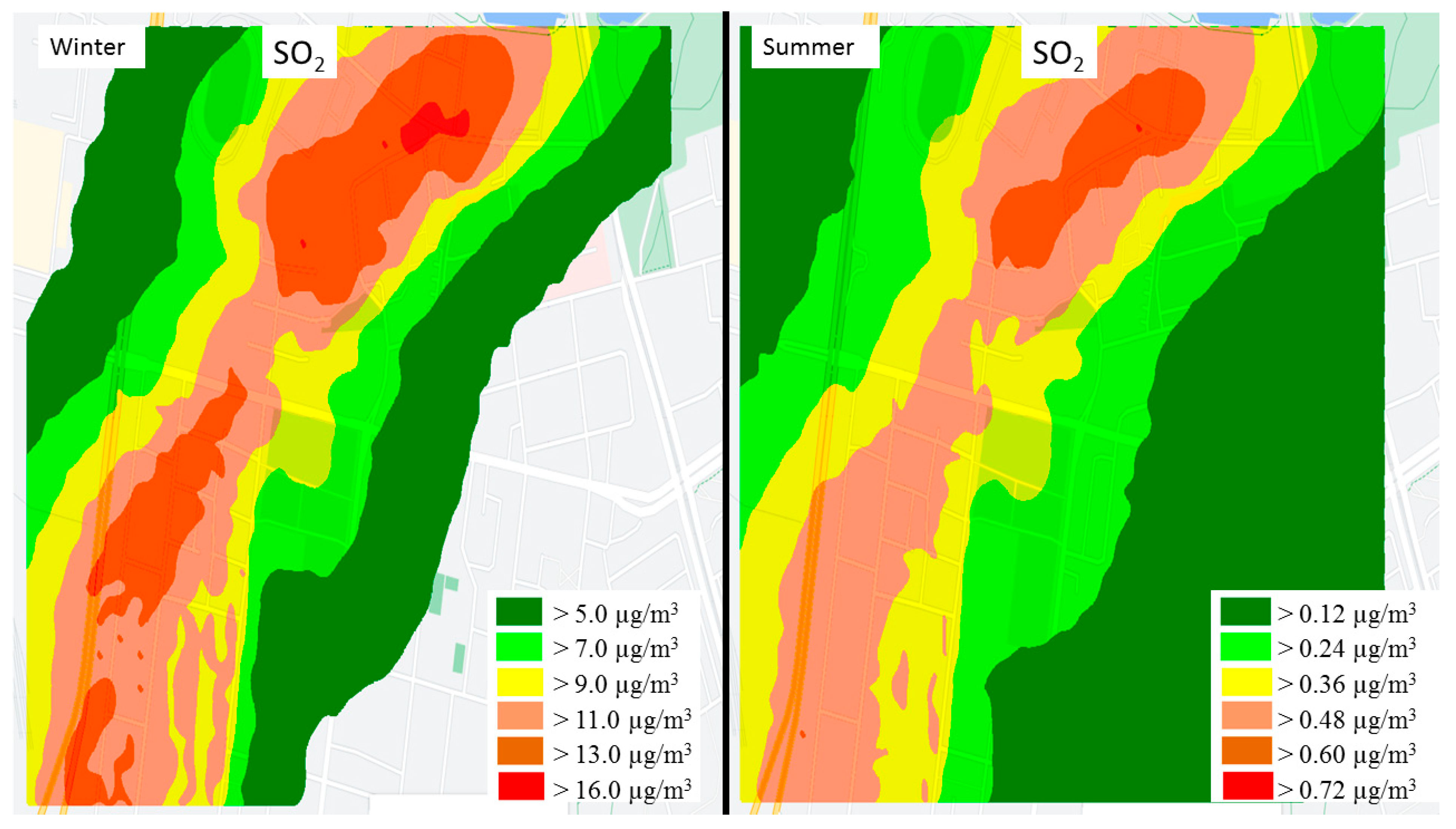
The emissions of pollutants selected in this study are mostly related to the combustion of fossil fuels. Therefore, SO2, which is another of the products of the combustion of fuels used in motor vehicles, was also included in the analysis. In series A of the winter period, the concentration of SO2 varied from 0.006 ppm to 0.346 ppm, i.e., from 20 µg/m3 to 970 µg/m3. Spatial analysis (Figure 6) showed the presence of an area with a high concentration of SO2 above 0.24 ppm (>670 µg/m3) at the sites of traffic jams before the eastern intersection. It may also be due to SO2 being transported downwind from industrial emitters such as EC3. The second place with a high concentration of SO2 was at the extreme western intersection. Concentrations of SO2 below 0.16 ppm (<450 µg/m3) were recorded only at a height of more than 30 m above ground level, in an area of low-rise single-family housing. This was probably due to the stronger ventilation in the area. According to the cross-section of the 3D dispersion map, the highest SO2 concentrations above 0.24 ppm were measured at ground level. With increasing heights above ground level, the concentration of SO2 decreased up to threefold. This suggests that the main sources of SO2 were car exhaust fumes and exhaust fumes from individual heating systems (single-family buildings). According to the EU, 15% of SO2 emissions are caused by individual heating systems [2]. Across the entire area, at a height of 2 m the permissible level of SO2 (350 µg/m3) according to EU standards [4] was exceeded by about 20–277%.
In the summer period, the SO2 concentration decreased significantly, and was up to three times lower compared to the winter period. In series C (Figure 6), the concentration of SO2 ranged from 0.001 ppm to 0.122 ppm (max 320 µg/m3). Similar to the winter period, the spatial distribution showed the presence of areas with increased SO2 concentrations at the intersections and the sites of traffic congestion. However, according to the cross-section of the pollution dispersion map, in summer the highest concentration of SO2 was not at ground level, as it was in winter. This can be explained by the fact that there was no thermal inversion in the summer period. This prevented the accumulation of pollutants and enabled faster mixing (dilution) in the atmospheric air. The concentration of SO2 was lowest at the highest point of the area of analysis and in the open space behind the crossing from the eastern side. This was probably related to the fact that these are zones of increased ventilation [31].
Finally, we considered the concentrations of Volatile Organic Compounds (Figure 7). In the winter and summer periods, the average VOCs concentration was about 20 µg/m3 (0.005 ppm). However, in the winter period the VOCs concentration reached 0.09–0.12 ppm (310–420 µg/m3), i.e., 53% higher than the maximum VOCs concentration in the summer period (0.023–0.079 ppm). This can be explained by a higher degree of photochemical reactions in the summer period, which reduce the concentration of VOCs. The cross-section of the pollution dispersion map for the winter months shows that the highest concentrations of VOCs were recorded close to the ground surface. As the altitude increased, the VOCs concentration quickly decreased to levels below 0.005 ppm (20 µg/m3). In summer, the highest concentrations of VOCs pollution occurred in the area around Pojezierska Street and towards the western intersection, where the heat and power plant is located. Xu et al. similarly identified a heat and power plant as the main origin of VOCs [32].
Table 2 presents the results of actual measurements from the representative series (A–D) taken during the 3 months of research in the winter and summer periods. The data show that in the winter period the concentration of particulate matter was almost four times higher relative to the average value than in the summer period. The concentration of SO2 was three times higher in the winter than in the summer. The average VOCs concentration remained at a similar level, regardless of the season.
The next part of the analysis used numerical software to calculate the dispersion of selected pollutants in relation to their probable sources of emissions.
The area of interest includes a heat and power plant with a chimney 120 m tall, from which emissions are released. Data were obtained from Veolia Energia Łódź, comprising a collective measurement of emissions (kg/h) from the chimney after desulphurization and dedusting of flue gases from five boilers. As can be seen in Table 3, the emissions were mostly composed of SO2 (despite the exhaust gas treatment systems). This suggests that the EC-3 CHP plant may be responsible for the high concentrations of SO2 found in our analysis.
Based on the parameters of the emitter and the amounts of pollutants, OPA03 software was used to simulate the dispersion of emissions from the EC-3 CHP plant. The results are shown in Figure 8, Figure 9, Figure 10, Figure 11 and Figure 12. According to the simulation, in winter, the maximum concentration of PM10 emitted from EC-3 was 0.21 µg/m3 (Figure 8).
In summer, the maximum concentration of PM10 according to our simulation was 0.42 µg/m3, i.e., twice as high as in the winter period. This can be explained by the exhaust velocity from the chimney in the summer period, which at 5.24 m/s was three times lower than in the winter period (16.2 m/s). A slower exhaust outlet in the summer period allows for faster precipitation of pollutants, and this results in a higher concentration of dust pollutants in the vicinity of the heat and power plant. However, in both the winter and summer periods the concentration of PM10 caused by the emission from EC-3 did not exceed 0.5 µg/m3 at a height of 2 m, which is less than 1% of the permissible value (50 µg/m3).
The analysis shows that SO2 was emitted from the CHP plant at a higher concentration than PM10 (Figure 9). In the winter period, the highest one-hour concentration according to the simulation was 20.35 µg/m3. This value occurred in the immediate vicinity of EC-3, covering the entire area of the analyzed street. At a distance of about 2 km from the CHP plant, the concentration of SO2 decreased to between 15 µg/m3 and 20 µg/m3. At a distance of about 6 km, it fell to below 15 µg/m3. In the summer period, the scope of the EC-3′s environmental impact area was reduced by about 16%, which translated into a higher concentration than 25 µg/m3 of SO2 within a 1 km radius of EC-3. Based on computer simulations, Lee et al. [7] also observed higher SO2 concentrations in the summer period, which were also explained by the lower outlet velocity in the summer period compared to the winter period. This resulted in a greater accumulation of pollution in the immediate vicinity of the heat and power plant.
The permissible maximum one-hour concentration of SO2 in the air is 350 µg/m3 [4]. The emissions of SO2 from the combined heat and power plant amounted to only 8.9% of the limit value in the summer period and to 5.8% in the winter period.
According to traffic volume studies carried out during the air quality measurements, an average of 983 vehicles per hour traveled between the west and the east intersections in the winter period, at an average speed of 32 km/h. In the summer period, the intensity increased by 14% to 1118 vehicles per hour. The average vehicle speed increased to approximately 39 km/h. The analyzed street was used mainly by passenger cars, which accounted for 89% (summer period) and 91% (winter period) of the total number of vehicles. Light trucks accounted for 8% or 7% of the traffic in each period, trucks for 2% or 1%, and public buses for 1%. These results were used to create a numerical simulation in the OPA03 program of the dispersion of linear pollutants (Figure 10 and Figure 11). Comparing the simulations of PM10 dispersion in the summer and winter periods (Figure 10), it can be observed that in the summer period there were higher concentrations of PM10 emissions. In the winter period, the maximum one-hour concentration was 12 µg/m3, whereas in the summer period it was 17.7 µg/m3. This was related to a 14% higher number of vehicles in the summer season, with a simultaneous increase in speed of only 7 km/h compared to the winter period. According to the simulation, the emissions from vehicle traffic had a small range of influence, as they were limited mainly to the immediate area of the street. This was due to the densely built-up area and the presence of tree stands (15–30 m tall trees). As Long et al. observed [27], local rough terrain has an impact on local meteorological conditions, especially in terms of wind direction and speed. Highly rough terrain contributes to protection against low windspeed and reduced airing, reducing the accumulation of pollutants. According to the simulation, the maximum concentration of PM10 was 35.4% of the permissible average daily concentration of 50 µg/m3 [4].
The spatial distribution of SO2 (Figure 11) according to the simulation was similar to the data for particulate matter. It was concentrated mainly in the road area and a small area of the surroundings (about 40 m). According to the simulations, the highest concentrations of SO2 occurred within the lanes of the road, reaching 43.5 µg/m3 in winter and 52.3 µg/m3 in summer. In the area of the pedestrian sidewalks, the one-hour concentration decreased to below 15 µg/m3. Road traffic emissions were at 12.4% of the maximum permissible level of 350 µg/m3 stipulated by the EU [4] in winter and 14.9% of the maximum in summer.
In the immediate vicinity of the analyzed street, there are about 170 single-family houses with individual heating systems (70% coal fired and 30% natural gas). Based on detailed data in the literature on this source of emissions [33], presented in Table 4, calculations were made in the OPA03 program for point emitters located using the map of the analyzed area (Figure 2).
There was a visible difference between the summer and winter periods in terms of the concentrations of PM10 and SO2 (Figure 12 and Figure 13). Therefore, different scales were used in the figures to present the results. During the summer period, the PM10 concentration (hourly maximum) (Figure 12) fluctuated between 0.03 µg/m3 and 0.161 µg/m3, because the heating systems were used mainly for the purpose of preparing domestic hot water. In the winter period, the concentration of PM10 emitted from individual heating systems was higher than the highest value calculated in the summer period, ranging from 0.6 µg/m3 to 4.0 µg/m3. This can be explained by the increased combustion of fuels for the production of thermal energy to heat the buildings in winter. Kaczmarczyk et al. [8] and Specjał et al. [34] made similar observations.
The concentration of SO2 in the summer was more than 10 times lower than in the winter period, when there is increased production of heat energy. According to the results presented in Figure 13, in the summer period the maximum hourly SO2 concentration varied in the range of 0.12–0.72 µg/m3, whereas in the winter period it was in the range of 5.0–16.0 µg/m3. The maximum value calculated in the summer period was 0.2% of the permissible value, and in the winter period it was 4.6% of the permissible value (350 µg/m3).
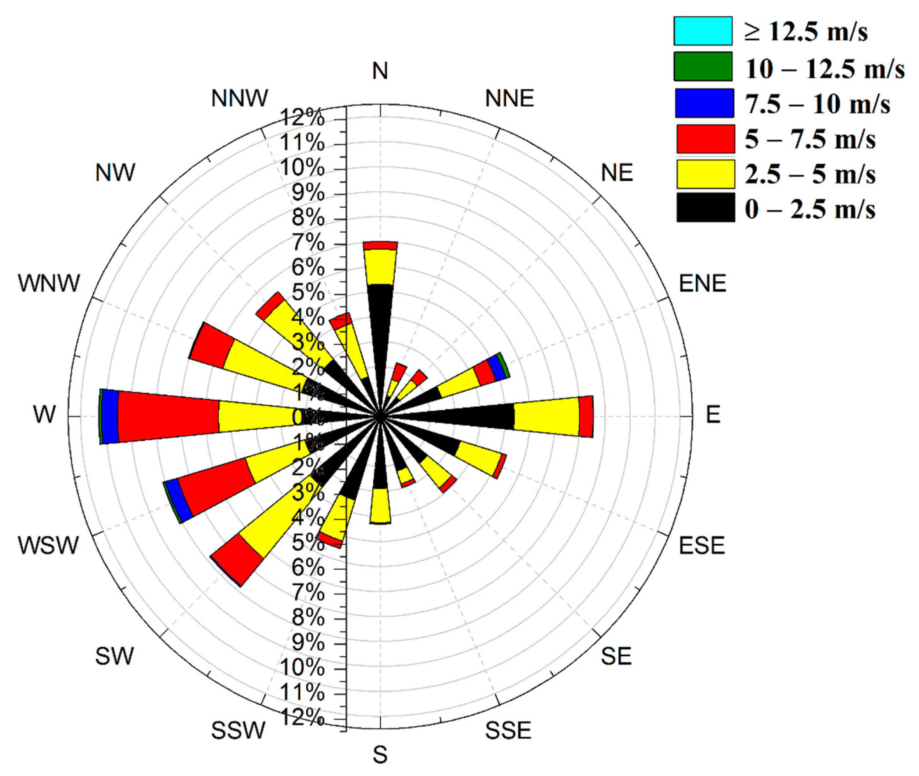
The pollution from individual heating systems depended strongly on local factors, especially the wind direction. The highest concentrations of PM10 and SO2 recorded in the axis of the location of the emitters, as the pollutants moved mainly in the direction of the WSW wind, which is dominant in the area. As a result, the emissions from individual heat sources did not affect the whole area of the analyzed street, but only the part in the direction of the wind.

4. Conclusions

In this study, we have compared the results of simulations performed using numerical software with data from actual field measurements. Maps were created of the distributions of air pollution in the vicinity of a heat and power plant and a communication route. For the numerical simulations, we assumed the highest concentrations of emissions from the selected pollution sources. According to the simulations, in the winter and summer periods, the maximum concentrations of PM10 were 16.22 µg/m3 and 18.29 µg/m3, respectively. According to our actual measurements, the maximum hourly concentration was in winter about 58.8 µg/m3 and in summer 23.5 µg/m3. The difference between the results of the simulation and the actual concentration of PM10 indicates the possibility of an additional source of dust pollution not included in the study, or the influence of background pollutants transported by the wind. There may also have been calculation errors associated with our method.
According to the simulation data shown in Figure 14, road transport accounted for the largest percentages of total PM10 emissions, at around 74% in winter and 96.9% in summer. The CHP was responsible for the smallest share of PM10 emissions, amounting to 1.3% or 2.3% of the total emissions according to the numerical calculations. This was related to the legal restrictions on dust emissions from power plants and the use of modern flue gas cleaning systems. The total maximum concentrations of SO2 according to the numerical calculations were 81.0 µg/m3 in winter and 84.0 µg/m3 in summer. The concentration of SO2 according to the actual measurements was about 350% higher than in the simulation for the winter period and about 140% higher than in the simulation for the summer period. Similar differences between real measurements and the results of simulations were reported by [7]. As in the case of PM10, it can be explained by the high concentrations of pollutants transported by the air close to the ground surface, especially in winter during so-called thermal inversion. This causes the phenomenon of smog in the winter (poor air quality), as demonstrated by Wielgosiński et al. [35]. The vertical cross-sections through the dispersion maps of pollutants in winter (Figure 4, Figure 6 and Figure 7) showed the highest concentrations close to the ground level (approx. 2 m).
According to the calculations performed by the OPA03 program (Figure 14), most emissions of SO2 were caused by road transport, which was responsible for 53.8% and 62.2% of the total maximum concentrations in winter and summer, respectively. Road transport has a particularly strong impact on air quality in densely populated areas [36], where vehicles generate much higher concentrations of pollutants due to slow traffic and high vehicle aggregation with little airflow [37]. This is especially important in Poland where, according to comparative studies, the air quality is worse than in other European Union countries [38]. According to data from the European Union [2] and Poland [28], road transport is one of the main sources of PM and gas emissions. Individual heating systems were responsible for the smallest share of SO2 emissions, amounting to 21.1% in winter and 0.8% of total emissions in summer. Similarly, Kaczmarczyk et al. [8] reported that individual heating systems were primarily responsible for the emission of particulate matter, especially when hard coal was used as fuel. Comparing the results from numerical calculations with the actual measurements shows the importance of using mobile measuring devices in air quality analyses, because simulations do not take into account all potential sources of air pollution or the correct level of background pollution. The presented research methodology can be implemented in any urban area, with a particular focus on local scale analysis.

Author Contributions

Conceptualization, R.C. and M.D.; methodology, R.C., M.D.; software, M.D., R.C.; writing—original draft, R.C., M.D.; review and editing, R.C. All authors have read and agreed to the published version of the manuscript.

Funding

This study was conducted as part of the research project entitled “Spatial analysis of air pollution changes in the Lodz agglomeration (in Polish: Analiza przestrzenna zmian stanu zanieczyszczenia powietrza w aglomeracji łódzkiej)”, which was co-financed approx. 80% by the Provincial Fund for Environmental Protection and Water Management in Łódź (in Polish: Wojewódzki Fundusz Ochrony Środowiska i Gospodarki Wodnej w Łodzi).

Institutional Review Board Statement

Not applicable

Informed Consent Statement

Not applicable.

Data Availability Statement

Data available on request.

Conflicts of Interest

The authors declare no conflict of interest.

References

  1. European Commission’s Joint Research Centre (JRS). Available online: https://ghsl.jrc.ec.europa.eu/ (accessed on 12 September 2021).
  2. Air Quality in Europe—2020 Report. Available online: https://www.eea.europa.eu/publications/air-quality-in-europe-2020-report (accessed on 12 September 2021).
  3. World Health Organization. WHO Air Quality Guidelines for Particulate Matter, Ozone, Nitrogen Dioxide and Sulfur Dioxide. Global Update 2005; Summary of Risk Assessment; World Health Organization: Geneva, Switzerland, 2005; Available online: https://www.euro.who.int/en/health-topics/environment-and-health/air-quality/publications/pre2009/air-quality-guidelines.-global-update-2005.-particulate-matter,-ozone,-nitrogen-dioxide-and-sulfur-dioxide (accessed on 2 June 2021).
  4. Legal Act of the European Union: Directive 2008/50/EC of the European Parliament and of the Council of 21 May 2008 on Ambient Air Quality and Cleaner Air for Europe OJ L 152; (BG, ES, CS, DA, DE, ET, EL, EN, FR, IT, LV, LT, HU, MT, NL, PL, PT, RO, SK, SL, FI, SV) Special edition in Croatian: 11 June 2008; 2008; Volume 29, Chapter 15, pp. 169–212. Available online: http://data.europa.eu/eli/dir/2008/50/oj (accessed on 2 August 2021).
  5. World Health Organization. WHO Global Air Quality Guidelines: Particulate Matter (PM2.5 and PM10), Ozone, Nitrogen Dioxide, Sulfur Dioxide and Carbon Monoxide; World Health Organization: Geneva, Switzerland, 2021; Available online: https://apps.who.int/iris/handle/10665/345329 (accessed on 12 September 2021).
  6. Meng, M.; Zhou, J. Has air pollution emission level in the Beijing–Tianjin–Hebei region peaked? A panel data analysis. Ecol. Indic. 2020, 119, 106875. [Google Scholar] [CrossRef] [PubMed]
  7. Lee, H.; Yoo, J.; Kang, M.; Kang, J.; Jung, J.; Oh, K. Evaluation of concentrations and source contribution of PM 10 and SO 2 emitted from industrial complexes in Ulsan, Korea: Interfacing of the WRF–CALPUFF modeling tools. Atmos. Pollut. Res. 2014, 5, 664–676. [Google Scholar] [CrossRef] [Green Version]
  8. Kaczmarczyk, M.; Sowiżdżał, A.; Tomaszewska, B. Energetic and Environmental Aspects of Individual Heat Generation for Sustainable Development at a Local Scale—A Case Study from Poland. Energies 2020, 13, 454. [Google Scholar] [CrossRef] [Green Version]
  9. Batterman, S.; Ganguly, R.; Isakov, V.; Burke, J.; Arunachalam, S.; Snyder, M.; Robins, T.; Lewis, T. Dispersion Modeling of Traffic-Related Air Pollutant Exposures and Health Effects among Children with Asthma in Detroit, Michigan. Transp. Res. Rec. J. Transp. Res. Board 2014, 2452, 105–113. [Google Scholar] [CrossRef] [PubMed] [Green Version]
  10. Tsai, D.H.; Wang, J.L.; Chuang, K.J.; Chan, C.C. Traffic-related air pollution and cardiovascular mortality in central Taiwan. Sci. Total Environ. 2010, 408, 1818–1823. [Google Scholar] [CrossRef] [PubMed]
  11. Kuklinska, K.; Wolska, L.; Namiesnik, J. Air quality policy in the U.S. and the EU—A review. Atmos. Pollut. Res. 2015, 6, 129–137. [Google Scholar] [CrossRef]
  12. Air Quality e-Reporting. Available online: https://www.eea.europa.eu/data-and-maps/data/aqereporting-9 (accessed on 12 September 2021).
  13. Bossche, J.; Peters, J.; Verwaeren, J.; Botteldooren, D.; Theunis, J.; Baets, B. Mobile monitoring for mapping spatial variation in urban air quality: Development and validation of a methodology based on an extensive dataset. Atmos. Environ. 2015, 105, 148–161. [Google Scholar] [CrossRef] [Green Version]
  14. Cichowicz, R.; Dobrzański, M. 3D Spatial Analysis of Particulate Matter (PM10, PM2.5 and PM1.0) and Gaseous Pollutants (H2S, SO2 and VOC) in Urban Areas Surrounding a Large Heat and Power Plant. Energies 2021, 14, 4070. [Google Scholar] [CrossRef]
  15. Jumaah, H.J.; Kalantar, B.; Halin, A.A.; Mansor, S.; Ueda, N.; Jumaah, S.J. Development of UAV-Based PM2.5 Monitoring System. Drones 2021, 5, 60. [Google Scholar] [CrossRef]
  16. Kim, H.; Tae, S.; Zheng, P.; Kang, G.; Lee, H. Development of IoT-Based Particulate Matter Monitoring System for Construction Sites. Int. J. Environ. Res. Public Health 2021, 18, 11510. [Google Scholar] [CrossRef]
  17. Łatuszyńska, M.; Strulak-Wójcikiewicz, R. A model for assessing the environmental impact of transport. Oper. Res. Decis. 2013, 23, 67–80. [Google Scholar] [CrossRef]
  18. Abu-Allaban, M.; Abu-Qdais, H. Impact Assessment of Ambient Air Quality by Cement Industry: A Case Study in Jordan. Aerosol Air Qual. Res. 2011, 11, 802–810. [Google Scholar] [CrossRef]
  19. Paas, B.; Schneider, C. A comparison of model performance between ENVI-met and Austal2000 for particulate matter. Atmos. Environ. 2016, 145, 392–404. [Google Scholar] [CrossRef]
  20. Atamaleki, A.; Zarandi, S.M.; Fakhri, Y.; Mehrizi, E.A.; Hesam, G.; Faramarzi, M.; Darbandi, M. Estimation of air pollutants emission (PM10, CO, SO2 and NOx) during development of the industry using AUSTAL 2000 model: A new method for sustainable development. MethodsX 2019, 6, 1581–1590. [Google Scholar] [CrossRef]
  21. Kowalski, M.; Wiśniewski, S. Natężenie ruchu a zagospodarowanie Łodzi—zarys problematyki w świetle danych z Obszarowego Systemu Sterowania Ruchem. Pr. Kom. Geogr. Komun. PTG 2017, 20, 20–36. [Google Scholar] [CrossRef] [Green Version]
  22. Technical Data of the EC-3 Heat and Power Plant. Available online: https://energiadlalodzi.pl/dane-kluczowe/dane-techniczne/ (accessed on 2 August 2021).
  23. ArcGis Software for Creating Dispersion Maps. Available online: https://www.arcgis.com/index.html (accessed on 2 August 2021).
  24. Calculation Software for Pollutant Concentration Analysis. Available online: http://www.eko-soft.com.pl/sysopa.htm (accessed on 2 June 2021).
  25. Cichowicz, R.; Dobrzański, M. Modeling Pollutant Emissions: Influence of Two Heat and Power Plants on Urban Air Quality. Energies 2021, 14, 5218. [Google Scholar] [CrossRef]
  26. Polish Legal Act. Rozporządzenie Ministra Środowiska z Dnia 26 Stycznia 2010 r. w Sprawie Wartości Odniesienia dla Niektórych Substancji w Powietrzu. Available online: http://isap.sejm.gov.pl/isap.nsf/DocDetails.xsp?id=wdu20100160087 (accessed on 2 June 2021).
  27. Long, P.; Enjian, Y.; Yang, Y. Impact analysis of traffic-related air pollution based on real-time traffic and basic meteorological information. J. Environ. Manag. 2016, 183, 510–520. [Google Scholar] [CrossRef]
  28. Centrum Badań i Edukacji Statystycznej GUS. Development of the Methodology and Estimation of the External Costs of Air Pollution Emitted from Road Transport at National Level; Final report; Centrum Badań i Edukacji Statystycznej GUS: Warszawa, Poland, 2018. Available online: http://stat.gov.pl (accessed on 12 August 2021).
  29. Meteorological Data. Available online: https://danepubliczne.imgw.pl/ (accessed on 12 September 2021).
  30. Polish Air Quality Index. Available online: https://powietrze.gios.gov.pl/pjp/current (accessed on 12 August 2021).
  31. Badach, J.; Voordeckers, D.; Nyka, L.; Van Acker, M. A framework for Air Quality Management Zones—Useful GIS-based tool for urban planning: Case studies in Antwerp and Gdańsk. Build. Environ. 2020, 174, 106743. [Google Scholar] [CrossRef]
  32. Xu, Y.; Yu, H.; Yan, Y.; Peng, L.; Li, R.; Wang, C.; Li, Z. Emission Characteristics of Volatile Organic Compounds from Typical Coal Utilization Sources: A Case Study in Shanxi of Northern China. Aerosol Air Qual. Res. 2021, 21, 210050. [Google Scholar] [CrossRef]
  33. Instytut Chemicznej Przeróbki Węgla. Wskaźniki Emisji Zanieczyszczeń Powietrza Emitowanych z Indywidualnych Źródeł Ciepła—Raport. Available online: http://czysteogrzewanie.pl/wp-content/uploads/2013/02/Wska%C5%BAniki-emisji-zanieczyszcze%C5%84-powietrza-emitowanych-z-indywidualnych-%C5%BAr%C3%B3de%C5%82-ciep%C5%82a-Raport.pdf (accessed on 12 September 2021).
  34. Specjał, A.; Lipczyńska, A.; Hurnik, M.; Król, M.; Palmowska, A.; Popiołek, Z. Case Study of Thermal Diagnostics of Single-Family House in Temperate Climate. Energies 2019, 12, 4549. [Google Scholar] [CrossRef] [Green Version]
  35. Wielgosiński, G.; Czerwinska, J.; Namiecińska, O.; Cichowicz, R. Smog episodes in the Lodz agglomeration in the years 2014–2017. In The E3S Web of Conferences; EDP Sciences: Ulysse, France, 2018; p. 01039. [Google Scholar] [CrossRef] [Green Version]
  36. Amirjamshidi, G.; Mostafa, T.S.; Misra, A.; Roorda, M.J. Integrated model for microsimulating vehicle emissions, pollutant dispersion and population expo-sure. Transp. Res. Part D Transp. Environ. 2013, 18, 16–24. [Google Scholar] [CrossRef]
  37. Yao, E.; Song, Y. Study on eco-route planning algorithm and environmental impact assessment. J. Intell. Transp. Syst. Technol. Plan. Oper. 2013, 17, 42–53. [Google Scholar] [CrossRef]
  38. Cichowicz, R.; Wielgosiński, G. Analysis of Variations in Air Pollution Fields in Selected Cities in Poland and Germany. Ecol. Chem. Eng. 2018, 25, 217–227. [Google Scholar] [CrossRef] [Green Version]
Figure 1. Location of the research area in the city of Łódź in Poland, Europe (photo background source: Google Earth Pro).
Energies 15 00553 g001
Figure 2. Map of the main areas affecting air quality: 1—analyzed area from the west intersection “I” to the east intersection “II”; 2—area of large-format stores; 3—green areas; 4—single-family houses; 5—multi-family houses; 6—industrial areas: warehouse, offices, small handicraft industries, and EC3 heat and power plant (photo background source: Google Earth Pro).
Energies 15 00553 g002
Figure 3. Wind rose for the city of Łódź in 2021 (own study based on data from source [29]).
Energies 15 00553 g003
Figure 4. Spatial distribution of PM10 concentrations during the winter season in series A and B.
Energies 15 00553 g004
Figure 5. Spatial distribution of PM10 concentrations during the summer season in series C and D.
Energies 15 00553 g005
Figure 6. Spatial distribution of SO2 concentrations during the winter season in series A and during the summer season in series C.
Energies 15 00553 g006
Figure 7. Spatial distribution of VOCs concentrations during the winter season in series A and during the summer season in series D.
Energies 15 00553 g007
Figure 8. Dispersion diagram of the maximum 1-h concentrations of PM10 emitted in the summer and winter periods from EC-3.
Energies 15 00553 g008
Figure 9. Dispersion diagram of the maximum 1-h concentrations of SO2 emitted in the summer and winter periods from EC-3.
Energies 15 00553 g009
Figure 10. Dispersion diagram of the maximum 1-h concentrations of PM10 emitted in the summer and winter periods from road traffic.
Energies 15 00553 g010
Figure 11. Dispersion diagram of the maximum 1-h SO2 concentration in the summer and winter periods from road traffic.
Energies 15 00553 g011
Figure 12. Dispersion diagram of the maximum 1-h PM10 concentrations of emissions from individual heating systems in the summer and winter periods.
Energies 15 00553 g012
Figure 13. Dispersion diagram of the maximum 1-h SO2 concentrations of emissions from individual heating systems in the summer and winter periods.
Energies 15 00553 g013
Figure 14. Percentage share of selected air pollution sources in the total maximum hourly concentrations of air pollutants in the summer and winter periods, based on numerical calculations.
Energies 15 00553 g014
Table 1. Meteorological data for representative measurement series during the winter and summer periods (source: [29]).
SeriesDate
Y.M.D
Temperature
[2 m Above Ground]
Relative Humidity
[2 m Above Ground]
Wind Speed
[10 m Above Ground]
Wind Direction
°C%m/s°
MinMeanMaxMinMeanMaxMinMeanMaxMean
A22 January 20213.269.466789112.84191
B25 February 2021−1.4717.439759711.33207
C24 June 202117.22228.3618110012.15190
D7 July 202118.42531.440658912.87167
Table 2. Measured concentrations of pollutants in a representative measurement series during the winter and summer periods in 2021.
WinterSummer
SeriesABCD
Date22 January 202125 February 202124 June 20217 July 2021
PM10
μg/m3
max42.3877.5416.0032.00
mean21.7954.808.2312.08
min11.2841.693.308.60
PM2.5
μg/m3
max36.6065.4015.0030.00
mean14.9838.625.2210.77
min4.8023.102.707.40
PM1
μg/m3
max36.5065.4010.0019.20
mean13.9837.593.709.12
min3.8022.101.106.40
VOCs
ppm
max0.0900.1220.0230.079
mean0.00490.005980.0050.022
min0.0010.0010.0010.001
SO2
ppm
max0.3460.2690.1640.122
mean0.2480.1310.0590.075
min0.0060.0080.0010.001
Table 3. Maximum hourly emissions of pollutants for the EC-3 CHP plant (own calculations based on data from Veolia Energia Łódź).
EmitterMaximum Hourly Emission [kg/h]
H120PM10PM2.5SO2
2.6671.143128.81
Table 4. Hourly emissions of pollutants from individual heating systems (source: [33]).
Source of HeatHourly Emission [g/GJ]
5-years-old or older boiler, automatically powered by fine coalPM10SO2
91.00343.00
Natural gas fired boiler0.300.40
Publisher’s Note: MDPI stays neutral with regard to jurisdictional claims in published maps and institutional affiliations.

