Differential Analysis of Fault Currents in a Power Distribution Feeder Using abc, αβ0, and dq0 Reference Frames

Abstract

This paper proposes a methodology to monitor the instantaneous value of the current and its derivative in the abc, αβ0, and dq0 reference frames to act in the detection of fault current in medium-voltage distribution systems. The method employed to calculate the derivative was Euler’s, with processing sampling rates of 10, 50, 100, and 200 μs. Using the MATLAB/Simulink platform, fault situations were analyzed on a real feeder of approximately 1.1132 km in length, fed by an 11.4 kV source, composed of 26 unbalanced loads and modeled as constant power. The simulation results show that the detection occurred in the different fault situations implemented in the feeder and that the detection speed is related to the value of the processing sampling rate (PSR) used. Considering all fault situations and regardless of the PSR value used, the total average detection time was 49 µs. Besides that, the joint action of the detection system with the Thyristor Controlled Series Capacitor (TCSC) limited the fault current in each situation. The average detection time for each fault situation analyzed was below the typical time for a recloser to act, regardless of the reference adopted for the analysis.

1. Introduction

Approximately 1 billion people worldwide currently live without access to electricity, and it is estimated that by 2030 about 780 million will remain in this condition. In recent years, this situation has improved mainly due to the development of technologies that have allowed access and participation in new forms of energy generation in the world electrical matrix. The old paradigm of access to energy through the expansion of the existing electrical system—centralized generation—has been overcome. Considering the recent increase of the energy demand, a new form of energy generation known as distributed generation (DG) is strongly recommended. DG allows the consumers to generate their own energy, with the possibility of injecting the surplus generated into the concessionaire’s network [1].

The growing presence of this type of generation in power systems requires a high level of protection to be able to detect and isolate failures that may occur in the different operation modes of the DG, in the least possible time while maintaining selectivity. This growth means that traditional systems, with centralized generation, tend to transform from radial unidirectional power flow networks into active networks in which the power flow can run in multiple directions, causing the short currents to change in value and direction [2]. Thus, to avoid loss of selectivity, the settings of the protection devices must be frequently checked as the installation of new DG units increases [3]. In addition to the loss of selectivity, the performance of the overcurrent relay, the coordination between fuse and recloser, and the operation in island mode, caused by the presence of the DG, can impact the distribution networks protection systems [4,5]. Alternative proposals are suggested to try to mitigate these impacts collaborating with the efficiency of protection systems: change of protection devices or adjustments; disconnection of the generation distributed during the faults; creating balance between the different technologies of DG; use of adaptive protection; use of intelligent transformers; using the fault current limiter (FCL) [5].

Among the alternatives listed, the use of an FCL is shown as one of the most efficient options in reducing the effects caused by the presence of the DG in the protection of distribution systems. Basically, it is a device formed by an impedance inserted in series with the circuit that is intended to limit the current and its value varies according to the current that circulates through the circuit. In normal conditions, the impedance value is approximately zero. If a fault is detected, it increases sharply in order to limit the short-circuit current. Once the fault is over, the impedance value returns to the normal condition [6].

The FCL eliminates the selectivity problem caused by the connection of new DG units without the need to readjust or replace the protection elements already installed. Moreover, the use of FCL results in an increase in the reliability and safety of the system, improvement in the transient stability, mitigation of voltage sags at the common coupling point, improvement of the system’s capacity, and increase in the integration of DG in the distribution [7,8,9].

Regarding the desirable electrical characteristics of an FCL, the following stand out: low impedance under nominal system operating conditions; limitation of the first peak of the transient fault current; limitation of the stationary fault current; no action under sufficiently small fault currents; capacity for many maintenance-free operations; high reliability and long service life; no overvoltages arising from current limitation; fast and automatic return to the low-impedance state after the fault interruption; and low energy dissipation during the limiting action [9,10].

Among the main technologies currently used in the manufacture of FCL, specialized literature highlights the high-temperature superconducting fault current limiters, resonant fault current limiters, and solid-state fault limiters [10,11]. Depending on the type of technology used, the fault current will behave differently. The analysis of the limiter performance with a superconductor must consider thermal models and the type of material used as well. Regarding the resonant limiter, it has a high limiting action since the first cycles in which the fault occurs gradually limit the current until reaching the maximum value defined in the project. The solid-state current limiter (SSFCL) has a constant limiting action from the second cycle on which the fault is detected, but before detection, the current value is greater than the maximum specified current [7,12].

The SSFCL is a device that uses the switching of high-power semiconductors to interrupt the fault current before it reaches its maximum value. It maintains the network protection system coordination and can be installed in microgrids or in feeders with renewable sources. Faster semiconductor devices with a higher blocking voltage are required for this [8,13].

According to the scientific literature [14], Ueda was the pioneer in the development of the first SSFCL to be used in a distribution system. The arrangement consisted of gate turn-off thyristors (GTOs), current-limiting impedance, voltage limiting, and a fault current detector element. Each unit of the prototype tested had as voltage and current characteristics, respectively, 2 kV_RMS and 400 A_RMS. To be tested in a 6.6 kV distribution substation, it was necessary to associate units in series. The time between fault detection and its interruption was 40 µs.

Traditional protection devices use the fundamental phasors of the current and voltage signals to monitor the behavior of electrical systems. This procedure suffers a delay caused by data windowing, a characteristic of the algorithms used in phasor extraction [15]. As a result, research has been initiated to develop fast protection devices based on processing instantaneous quantities and to avoid phasor estimation procedures. Great scientific and industrial contributions, directed toward the development of time domain protection devices, took place in the 1980s. Hardware limitations, speed of response of algorithms, and the control of processed quantities in the time domain have been obstacles that have slowed the development of the area of fast protections. Significant contributions in this area have resumed since the 2000s [16].

Thus, research has been developed with the aim of improving a technology in the time domain that uses the instantaneous value of current and/or voltage, with no need for phasor calculation. As a result, the activation time of the protection devices is between 1 and 4 ms, which is difficult to achieve with phasor-based relays.

A method that is based on the analytical model of distribution systems and that uses effective values of current and voltage fundamental components referring to transients obtained at substations was proposed by [17]. Tests were performed using MATLAB/Simulink software to simulate the missing system, and it showed high accuracy.

A protection function based on the analysis of incremental quantities is presented in [18]. Using current and voltage signals obtained in the pre-fault condition and incremental current and voltage quantities, operating and restraining voltages in the protection range are estimated. By comparing these values, it is possible to determine whether the fault is internal or external to the considered protection zone. In an attempt to reduce the effects that the high-frequency components have on the algorithm, average values of operating magnitude are counted and considered for the relay actuation. Hence, average actuation times close to 12 ms are observed.

In order to promote faster actuation times and make the algorithm safer and more robust, [19] proposed a protection function that uses Clarke transform together with a frequency response compensation filter of the capacitive potential transformers.

Some functions intended for transmission line protection in the time domain, based on the use of incremental quantities and traveling wave theory, are proposed by [20]. Among these functions, the following stand out: directional power functions based on traveling waves and incremental quantities, distance function founded on the analysis of incremental quantities, and a function based on traveling wave theory.

The first transmission line protection device to employ only time-domain functions, based on incremental quantities and traveling wave theories, was presented by [21]. They displayed the main constructive details of the hardware and showed its operation in real fault situations and through simulations. Performance analysis is done by comparison with traditional phase-based protection devices. In all the tests performed, the device in the time domain was faster than traditional devices, showing an operation time of less than or equal to 20 ms.

Due to the emergence of new ultra-high-speed protection devices based on incremental quantities and traveling waves, configuration adjustments are required. Most often, these adjustments are related to the levels of incremental quantities and propagation times of the traveling waves. Then, for the setup to be done properly, it is necessary to know how to calculate incremental currents and voltages and how to estimate and measure the propagation times of the traveling waves [22].

A communications-based protection scheme that uses incremental-quantity directional elements and traveling waves to make decisions to shut down a transmission line, where voltage transformers with a coupling capacitor provide voltage signals to these elements is presented in [23]. Incremental-quantity directional elements operated in the range of 1055 to 8750 ms, with an average operating time of 2966 ms. The traveling-wave-based directional elements operated in the range of 105 µs and the slowest one was at 138 µs, with an average operating time of 116 µs. The details of the commissioning of two ultra-high-speed protection relays in the time domain from the pilot project developed in India are presented in [24]. They are installed on a hybrid line, 220 kV, 89 km long, and use incremental quantities of voltage and current, which are the differences between an instantaneous current sample and a sample from a previous cycle. Incremental quantities contain purely fault voltage and current, excluding any charge information. These signals are filtered in a low-pass filter, and then applied to directional and distance elements.

The high participation of DG in power systems, especially in distribution, has detrimental effects on the quality of power, causing losses for consumers and utilities.

In [25] a modified multi-class support vector machines (MMC-SVMs) technique is proposed to detect and identify faults, using the real-time RMS voltage values of each bar of the distribution system. These values are grouped into two dataset matrices: matrix showing no fault conditions; matrix associated with the fault conditions.

A method to detect and classify faults in distribution networks with the presence of DG is presented in [26]. Its main idea is to consider the operation modes of distributed generators in the analysis of fault characteristics using the Fortescue approach. In addition, SoftMax regression is employed to minimize the negative effects of transients on fault classification.

The authors of [27] present a fault detection method that uses a summarized matrix of the characteristics of the power system, RMS voltage information provided by the Hilbert transform, harmonic information obtained by the discrete Fourier transform, and a detection method based on the Hilbert–Huang transform. A typical 10.5 kV radial distribution network with three feeders is used to demonstrate, through simulations, the performance of the proposed fault detection method compared to several classical methods.

To limit the short-circuit current in a 500 kV AC main, an FCL based on a high-coupled split reactor (HCSR), namely, HCSR-FCL is proposed in [28]. The device is controlled in real time through a detection algorithm based on the squared ratio of the three-phase current, with two data windows as detection criteria. The simulation results showed that the fault detection time was below 1 ms.

In reference [29], a harmonic mitigation method to improve power quality in distribution systems is presented. It basically consists of the use of single-tuned harmonic filters (STFs), to minimize total harmonic distortion (THD) and power loss and improve the voltage profile considering different restrictions to meet the IEEE 519 standard. The Water Cycle algorithm (WCA) is used to determine the quantity, characteristics, and the installation location of STFs.

A method for fault detection in distribution systems with the presence of non-linear loads is presented in [30]. The phase angle of the third harmonic is obtained using the Stockwell transform and then compared to a self-adaptive threshold. An index based on the cumulative error generated by this comparison is employed to monitor the status of each phase.

Considering that the fault detection systems, especially the algorithms, used by the manufacturers of protection devices, are not open, that is, in the public domain, the development of the protection area is hindered. Thus, the focus of this study is to propose and analyze a system that works with instantaneous values of the current and its derivative to act quickly in detecting fault current in medium-voltage distribution systems.

The main contributions of this paper can be summarized as follows:

−

simplicity of the methodology;

−

monitoring in the time domain of the behavior of the instantaneous value of the current and its derivative, allowing an increase in the detection speed;

−

demonstration that the simultaneous monitoring of the current in three different references frames working together makes faster fault detection possible in many situations. The complementary action of the references in the detection of the fault causes the activation of the protection device to be made by a control signal issued by the reference that detects the fault first.

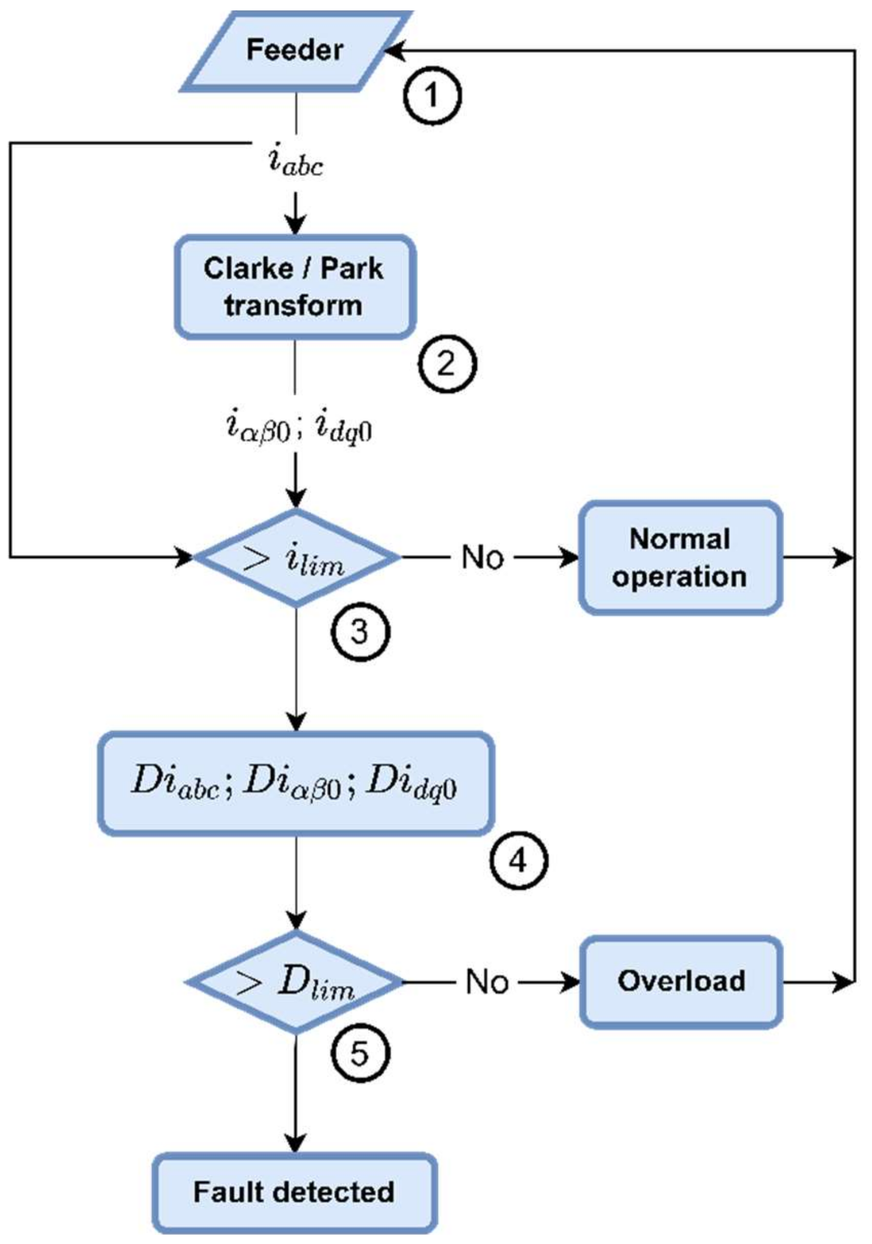
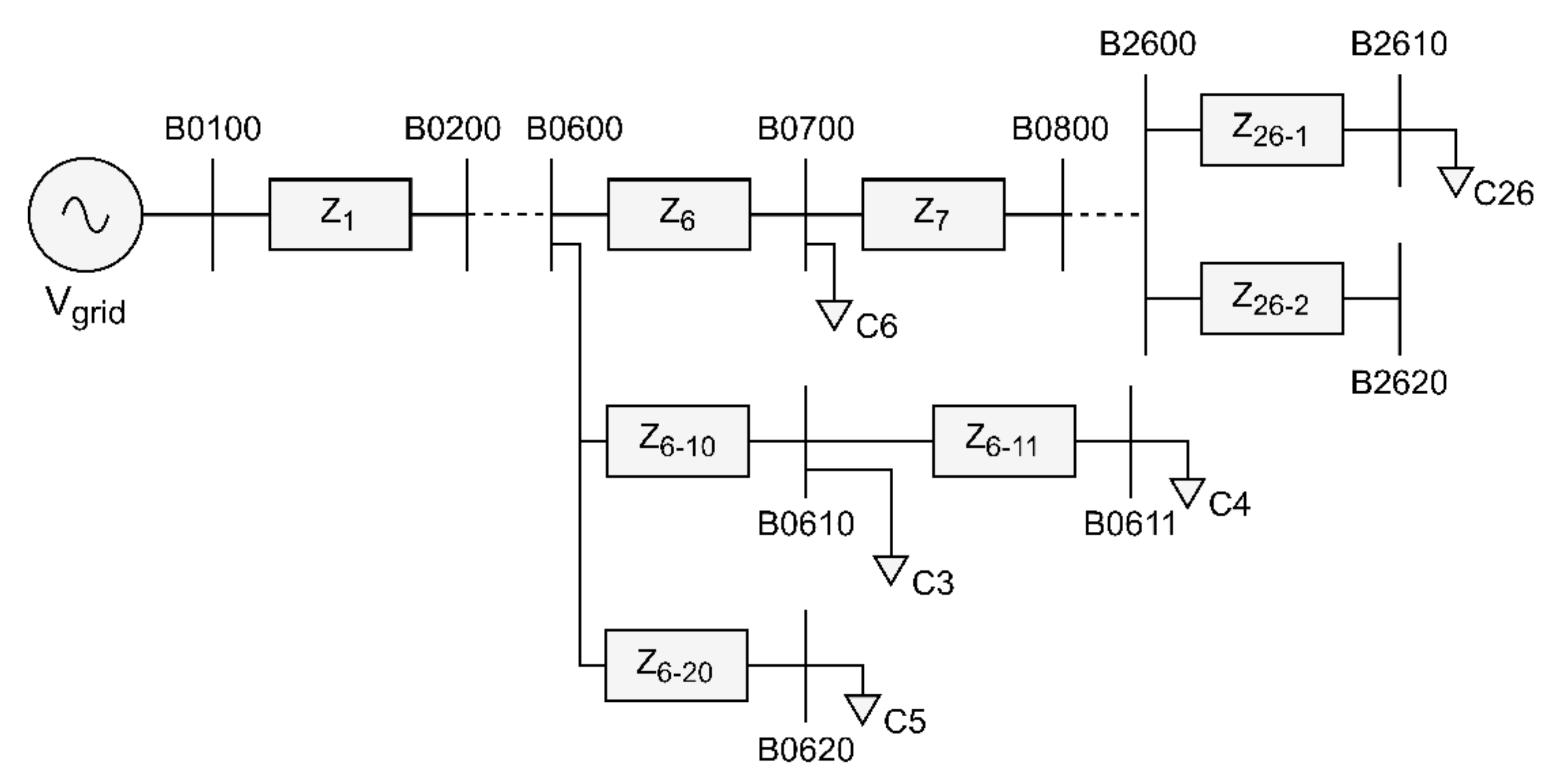
The structure of the paper is as follows: Section 2 presents the signal-processing-based fault detection techniques used in power systems; Section 3 presents the proposed fault current detection algorithm in the time domain; Section 4 presents a case study on a feeder belonging to a medium-voltage distribution system of a real network in the state of Espírito Santo, Brazil; Section 5 presents the simulation results obtained in abc, αβ0, and dq0 references, for different fault conditions and processing sampling rates; Section 6 presents a discussion; finally, Section 7 presents the conclusions.

2. A Fault Detection Techniques Based on Digital Signal Processing Used in Power Systems

2.1. Mathematical Morphology

A protection scheme using the initial current traveling wave and mathematical morphology (MM) is presented in [31]. This scheme provides an ultra-fast response and can be adapted to various system operating modes, topologies, and fault and load conditions. Only low-bandwidth communication is required to achieve high-speed operation and a proper discrimination level in mesh networks. A fault detection and location scheme in a microgrid is proposed in [32], using MM and recursive least squares (RLS). In the fault detection/classification step, an expansion and median erosion filter is applied to the microgrid current signal. In the fault location step, using a differential equation obtained from the equivalent microgrid model, the RLS method is employed to estimate the fault location. MM is used to act on current signals to extract a differential characteristics vector that will be used in an intelligent differential protection scheme for a microgrid system [33].

2.2. Hilbert–Huang Transform

A differential protection scheme for the analysis of a non-stationary signal was proposed, using the Hilbert–Huang transform (HHT) [34]. HHT was used in the study of faults in transmission lines and their distribution and in microgrids [33]. An HHT associated with an approach based on machine learning (ML) was utilized specifically in the identification of faults in microgrids. The process starts with measuring the current at different locations and later applied the empirical detection method for calculation unlike the differential characteristics of intrinsic functions. These characteristics are then applied to the HHT as inputs to the ML model for fault identification and classification.

2.3. The Wavelet Transform

The wavelet transform (WT) allows the transient analysis of current and voltage signals through the decomposition and parameterization of these signals. Discrete (DWT) and continuous (CWT) wavelet transforms are used to decompose current and voltage signals, making known their characteristics in various frequency ranges [35]. This signal decomposition is a process in which a filter bank decomposes signals into multi-level coefficients and one-level approximation coefficients. The proposed detection and classification method uses the positive sequence components of the current measured at the common coupling point (PCC) to calculate the WT coefficients [36]. The method’s proposal is to find an optimal wavelet function that, combined with WT functions selected by particle examination optimization, can be used to detect transient signal failures. An approach that combines wavelet functions and ML for fault classification in microgrids is shown in [37].

2.4. The S Transform

The S transform (ST) allowing the joint representation of time–frequency with frequency-dependent resolution, using a scalable, mobile Gaussian window is shown in [35]. This representation shows the spectral characteristics of the current and voltage signals, allowing the detection and interpretation of transients. The ST was used in the pre-processing of current signals from a distribution feeder with microgrids to obtain system characteristics that later served as input conditions for a computational tool, based on the tree decision (TD) and fuzzy logic (FL), used to detect and classify faults [38]. A differential protection technique was proposed in [39], in which the feeder currents are measured at both ends and then pre-processed with the ST to generate time and frequency contours. Then, spectral energies in the time–frequency domain are calculated and later used to detect the fault condition.

2.5. The Fast Fourier Transform

The fast Fourier transform (FFT) is based on the considerable difference in its coefficients during symmetric fault conditions. A discrete Fourier transform (DFT)-based fault characteristic extractor was proposed to obtain amplitude, phase, and frequency information from current and voltage signals [38]. This information was used to determine each feeder’s status in the power system. An algorithm, combined with a directional element, was used to adjust a relay considering the microgrid operating modes [40]. The presented method used full-cycle DFT and half-cycle DFT (HCDFT) to remove the direct current component and harmonics to estimate the phasor elements [35]. HCDFT was used to calculate fundamental and harmonic phasors for fault type classification. The fundamental components of the current and voltage signals were determined by the full-cycle FFT. The authors of [41] proposed a method using the phasor and current sequence components as inputs to a FCL module for fault detection and classification.

2.6. Park and Clarke Transforms

In many three-phase signal applications, it is convenient to carry out a coordinate change from the stationary system abc to a system that simplifies mathematical models, such as the αβ0 frame or the dq0 frame. These changes are made through mathematical transformations known as Clarke transform and Park transform.

A technique that uses Park vector trajectory (PVT) is presented in [42], together with the HHT to analyze transients in the load current in the occurrence of a fault in the common coupling point. In fault events, there is a deformation of the PVT when compared to its shape under electrical power system normal conditions. Through the application of Park and WT, a technique for fault detection in microgrids was presented [43]. The proposal is to transform three-phase current or voltage signals into dq0 components to analyze their behavior during transient situations of the power system, in order to recognize patterns that help in recognizing a fault. Then, by filtering one of the dq0 components through the WT and isolating the frequencies of the band of interest, faults can be detected using the finite difference between the filtered signal samples. We found a detection method using Clarke transform, and ST was found to portray the characteristics of current and voltage signals in fault events [44]. These characteristics are used to achieve the detection, location, and characterization of faults. According to [45], this technique can be applied in situations where the microgrid topology is variable. Clarke transform is used to find a methodology for the analytical solution of asymmetric transients [46]. This requires specific theoretical work, as the direct application of the Clarke transform does not produce the diagonalization of the system matrices. Closed analytical solutions are obtained through the representation and interpretation of α, β, and 0 modal circuits obtained from the asymmetry of the phases.

2.6.1. Clarke Transformation

The Clark transformation (αβ0) transforms a current, represented in the abc system, to a system with three quadrature signals, where the αβ signals are sinusoidal and the other signal corresponds to the zero sequence. Thus, we move from a three-phase system to an equivalent two-phase system, with imaginary axis in β and real axis α orthogonal [47]. The transformation can be represented by the following matrix equation:

$$\left[i_{\alpha \beta 0}\right]=\left[T_{\alpha \beta 0}\right]·\left[i_{abc }\right]$$

(1)

The transformation matrix is given by [47]

$$\left[T_{\alpha \beta 0}\right]=\sqrt{\frac{2}{3}}\left[\begin{array}{ccc}1& \raisebox{1ex}{$-1$}\!\left/ \!\raisebox{-1ex}{$2$}\right.& \raisebox{1ex}{$-1$}\!\left/ \!\raisebox{-1ex}{$2$}\right.\\ 0& \raisebox{1ex}{$\sqrt{3}$}\!\left/ \!\raisebox{-1ex}{$2$}\right.& \raisebox{1ex}{$-\sqrt{3}$}\!\left/ \!\raisebox{-1ex}{$2$}\right.\\ \raisebox{1ex}{$\sqrt{2}$}\!\left/ \!\raisebox{-1ex}{$2$}\right.& \raisebox{1ex}{$\sqrt{2}$}\!\left/ \!\raisebox{-1ex}{$2$}\right.& \raisebox{1ex}{$\sqrt{2}$}\!\left/ \!\raisebox{-1ex}{$2$}\right.\end{array}\right]$$

(2)

Then, the signal can be represented in the αβ0 system as follows:

$$\left[\begin{array}{c}{i}_{\alpha }\\ i_{\beta }\\ i_0\end{array}\right]=\sqrt{\frac{2}{3}}\left[\begin{array}{ccc}1& \raisebox{1ex}{$-1$}\!\left/ \!\raisebox{-1ex}{$2$}\right.& \raisebox{1ex}{$-1$}\!\left/ \!\raisebox{-1ex}{$2$}\right.\\ 0& \raisebox{1ex}{$\sqrt{3}$}\!\left/ \!\raisebox{-1ex}{$2$}\right.& \raisebox{1ex}{$-\sqrt{3}$}\!\left/ \!\raisebox{-1ex}{$2$}\right.\\ \raisebox{1ex}{$\sqrt{2}$}\!\left/ \!\raisebox{-1ex}{$2$}\right.& \raisebox{1ex}{$\sqrt{2}$}\!\left/ \!\raisebox{-1ex}{$2$}\right.& \raisebox{1ex}{$\sqrt{2}$}\!\left/ \!\raisebox{-1ex}{$2$}\right.\end{array}\right].\left[\begin{array}{c}{i}_a\\ i_b\\ i_c\end{array}\right]$$

(3)

After applying the transform to the currents of a three-phase abc system, we have to ensure that

$$i_a{}^2+i_b{}^2+i_c{}^2=i_{\alpha }{}^2+i_{\beta }{}^2+i_0{}^2$$

(4)

In a balanced abc system, the component $i_{\alpha }$ is in phase with phase a of the abc reference, the $i_{\beta }$ component is in quadrature with $i_{\alpha }$ and $i_0=0$. Thus, the modulus resulting from the sum of $i_{\alpha }$ and $i_{\beta }$ is calculated using $\sqrt{i_{\alpha }{}^2+i_{\beta }{}^2}$ and is a constant value.

2.6.2. Park Transformation

As the processing of sinusoidal signals is more complex than that of constant signals, Park transformation (dq0) represents currents that were transformed from the abc system in a synchronous vector system [48]. The transformation can be written as follows:

$$\left[i_{dq0 }\right]=\left[T_{dq0 }\right]·\left[i_{abc}\right]$$

(5)

The direct transformation from the abc system to the dq0 is performed using the matrix below [48]:

$$\left[T_{dq0 }\right]=\sqrt{\frac{2}{3}} \left[\begin{array}{ccc}\cos \theta & \cos \left(\theta -\raisebox{1ex}{$2\pi $}\!\left/ \!\raisebox{-1ex}{$3$}\right.\right)& \cos \left(\theta +\raisebox{1ex}{$2\pi $}\!\left/ \!\raisebox{-1ex}{$3$}\right.\right)\\ -\sin \theta & -\sin \left(\theta -\raisebox{1ex}{$2\pi $}\!\left/ \!\raisebox{-1ex}{$3$}\right.\right)& -\sin \left(\theta +\raisebox{1ex}{$2\pi $}\!\left/ \!\raisebox{-1ex}{$3$}\right.\right)\\ \raisebox{1ex}{$\sqrt{2}$}\!\left/ \!\raisebox{-1ex}{$2$}\right.& \raisebox{1ex}{$\sqrt{2}$}\!\left/ \!\raisebox{-1ex}{$2$}\right.& \raisebox{1ex}{$\sqrt{2}$}\!\left/ \!\raisebox{-1ex}{$2$}\right.\end{array}\right]$$

(6)

Thus, the signal components in the dq0 system are calculated as follows:

$$\left[\begin{array}{c}{i}_d\\ i_q\\ i_0\end{array}\right]=\sqrt{\frac{2}{3}} \left[\begin{array}{ccc}\cos \theta & \cos \left(\theta -\raisebox{1ex}{$2\pi $}\!\left/ \!\raisebox{-1ex}{$3$}\right.\right)& \cos \left(\theta +\raisebox{1ex}{$2\pi $}\!\left/ \!\raisebox{-1ex}{$3$}\right.\right)\\ -\sin \theta & -\sin \left(\theta -\raisebox{1ex}{$2\pi $}\!\left/ \!\raisebox{-1ex}{$3$}\right.\right)& -\sin \left(\theta +\raisebox{1ex}{$2\pi $}\!\left/ \!\raisebox{-1ex}{$3$}\right.\right)\\ \raisebox{1ex}{$\sqrt{2}$}\!\left/ \!\raisebox{-1ex}{$2$}\right.& \raisebox{1ex}{$\sqrt{2}$}\!\left/ \!\raisebox{-1ex}{$2$}\right.& \raisebox{1ex}{$\sqrt{2}$}\!\left/ \!\raisebox{-1ex}{$2$}\right.\end{array}\right].\left[\begin{array}{c}{i}_a\\ i_b\\ i_c\end{array}\right]$$

(7)

Currents in the abc and dq0 systems are listed as follows:

$$i_a{}^2+i_b{}^2+i_c{}^2=i_d{}^2+i_q{}^2+i_0{}^2$$

(8)

In balanced three-phase systems, the d component is null, and the q component remains constant and equal to the peak value of the current abc.

3. The Proposed Fault Current Detection

Figure 1 presents a flowchart of the methodology used in this work to detect faults in a distribution system. The proposed methodology consists of the following steps:

−

Step 1: Measure the instantaneous currents in the stationary reference abc, at the location where the protection device that will receive the signal from the fault detector will be installed.

−

Step 2: Transform the measured currents to the αβ0 and dq0 references. This can be done with the help of Equations (3) and (7).

−

Step 3: Compare the currents represented in all references with the limit current ($i_{lim})$, obtained from Equation (9), defined for each reference. This limit considers the normal operating system condition, maximum rated current of the feeder $\left(i_m\right),$ and the permissible overcharge percentage $\left({\Delta }_{over}\right)$, if any, according to the transient behavior of the load.

$$i_{\lim }=i_m\left(1+\frac{{\Delta }_{over}}{100}\right)$$

(9)

−

Step 4: Calculate the derivative of the current at each reference, obtained from Equation (10) [49], using Euler’s method. This is done by subtracting the current measured value $\left[i_{\left(n-1\right)}\right]$, from its corresponding later value $\left[i_{\left(n\right)}\right]$, obtained according to the adopted processing sampling rate (PSR).

$$D=\frac{\left[i_{\left(n\right)}-i_{\left(n-1\right)}\right]}{PSR}$$

(10)

−

Step 5: Compare the derivative in each reference with its corresponding limit derivative ($D_{lim})$, obtained from Equation (11) [49].

$$D_{lim}=\frac{\left[i_{lim}-i_{\left(n\right)}\right]}{PSR}$$

(11)

4. Case Study

Figure 2 shows the single-line diagram of the studied system. It consists of a feeder of approximately 1.132 km in length, fed by an ideal 11.4 kV source, belonging to the medium-voltage distribution system of a real network in the state of Espírito Santo, Brazil, composed of 26 unbalanced loads installed along the feeder and modeled as constant power. The buses of the system are numbered sequentially starting with B0100.

In each section of the feeder, different impedances were employed according to the characteristic of each cable and length of the section, given in

Table 1. Characteristics of each feeder section.

Zn	Buses	Length (m)	INominal (A)	R1 (Ω/m)	X1 (Ω/m)	R0 (Ω/m)	X0 (Ω/m)
Z1	B0100–B0200	205.77	560	0.000891	0.00107	0.006302	0.002036
Z2	B0200–B0300	16.49	314	0.000197	0.000252	0.000693	0.001275
Z3	B0300–B0400	21.54	314	0.000197	0.000252	0.000693	0.001275
Z4	B0400–B0500	13.34	314	0.000197	0.000252	0.000693	0.001275
Z5	B0500–B0600	54.06	314	0.000591	0.000756	0.002079	0.003825
Z6	B0600–B0700	15.23	314	0.000197	0.000252	0.000693	0.001275
Z7	B0700–B0800	34.18	314	0.000197	0.000252	0.000693	0.001275
Z8	B0800–B0900	37.34	314	0.000197	0.000252	0.000693	0.001275
Z9	B0900–B1000	2.24	500	0.000190	0.000406	0.000693	0.001275
Z10	B1000–B1100	56.65	314	0.000394	0.000504	0.001386	0.002550
Z11	B1100–B1200	48.39	314	0.000394	0.000504	0.001386	0.002550
Z12	B1200–B1300	64.26	314	0.000394	0.000504	0.001386	0.002550
Z13	B1300–B1400	23.77	314	0.000197	0.000252	0.000693	0.001275
Z14	B1400–B1500	43.87	500	0.000380	0.000812	0.001386	0.002550
Z15	B1500–B1600	23.24	500	0.000190	0.000406	0.000693	0.001275
Z16	B1600–B1700	37.80	500	0.000190	0.000406	0.000693	0.001275
Z17	B1700–B1800	34.21	500	0.000190	0.000406	0.000693	0.001275
Z18	B1800–B1900	36.24	500	0.000190	0.000406	0.000693	0.001275
Z19	B1900–B2000	27.80	500	0.000190	0.000406	0.000693	0.001275
Z20	B2000–B2100	35.61	500	0.000190	0.000406	0.000693	0.001275
Z21	B2100–B2200	82.41	500	0.000570	0.001218	0.002079	0.003825
Z22	B2200–B2300	20.05	500	0.000190	0.000406	0.000693	0.001275
Z23	B2300–B2400	50.49	500	0.000380	0.000812	0.001386	0.002550
Z24	B2400–B2500	83.76	500	0.000570	0.001218	0.002079	0.003825
Z25	B2500–B2600	31.58	500	0.000190	0.000406	0.000693	0.001275
Z26-1	B2600–B2610	32.23	500	0.000190	0.000406	0.000693	0.001275

.

Appendix A presents information about the impedances of the branches connected to the feeder in Figure 2.

Table 2. Characteristics of the charges connected along the feeder.

		Phase A		Phase B		Phase C
Charge	Bus	P (kW)	Q (kVAr)	P (kW)	Q (kVAr)	P (kW)	Q (kVAr)
C1	B0300	24.38	10.38	24.78	10.55	25.17	10.72
C2	B0500	10.51	4.48	23.23	9.89	22.72	9.67
C3	B0610	39.01	16.62	44.06	18.77	39.72	16.92
C4	B0611	26.42	11.25	24.39	10.39	24.26	10.33
C5	B0620	17.96	7.65	17.23	7.34	7.28	3.10
C6	B0700	48.39	20.61	44.95	19.15	46.13	19.65
C7	B0810	40	17.04	40	17.04	40	17.04
C8	B1010	34.58	14.73	30.54	13.01	39.86	16.98
C9	B1020	15.21	6.48	15.21	6.48	15.21	6.48
C10	B1100	23.02	9.81	18.07	7.69	15.58	6.64
C11	B1210	34.12	14.53	56.28	23.98	49.48	21.08
C12	B1211	51.14	21.79	52.74	22.47	53.27	22.69
C13	B1300	21.63	9.21	16.77	7.14	18.76	7.99
C14	B1510	70.34	29.97	50.65	21.58	34.76	14.81
C15	B1710	49	20.87	49	20.87	49	20.87
C16	B1810	58.19	24.79	54.49	23.21	56.25	23.96
C17	B1910	104	44.30	104	44.30	104	44.30
C18	B1920	27.44	11.69	33.00	14.06	36.92	15.73
C19	B1921	42.21	17.98	40.24	17.14	34.76	14.81
C20	B2010	46.02	19.61	47.40	20.19	45.25	19.27
C21	B2100	34.84	14.84	30.79	13.12	28.72	12.24
C22	B2210	63.67	27.12	63.67	27.12	63.67	27.12
C23	B2300	0	−200	0	−200	0	−200
C24	B2410	89	37.91	89	37.91	89	37.91
C25	B2500	49.01	20.88	41.93	17.86	43.60	18.57
C26	B2610	31.67	13.49	31.67	13.49	31.67	13.49

Note: adapted from [50].

presents the total power demand values of the 26 charges connected along the feeder. The power distribution in the buses is diverse and unbalanced.

The thyristor-controlled series capacitor (TCSC) is a variable impedance composed of a capacitor in parallel with a thyristor-controlled reactor (TCR), which is formed by two thyristors in antiparallel and in series with an inductor [51]. Figure 3 shows the TCSC.

It is formed by inserting a capacitor of 225.7 μF and an inductor of 21.8 mH in each phase of the B0100 bus.

The detection system of Figure 1 and the performance of the TCSC in limiting fault current in situations implemented in the circuit of Figure 2 will be evaluated.

5. Results

5.1. The Detection Method

The next subsections show the results of the simulations performed in MATLAB/Simulink from the distribution feeder model in Figure 2, considering the occurrence of single line to ground (SLG), double line to ground (2LG), line-to-line (2L), and three phase to ground (3LG) faults at B2620, with the fault resistance (R_F) assuming the values of 0, 10, 20, and 40 Ω and the processing sampling rate (PSR) presuming the values of 10, 50, 100, and 200 μs. In addition, for all the references considered, the time intervals (∆t) that correspond to the moment between the occurrence of each fault and its detection are presented. In situations where there was no detection, ∆t was considered infinite (ꝏ).

5.1.1. PSR = 10 μs

Table 3. Fault detection on B2620 to PSR = 10 μs.

	SLG				2LG
	∆t0Ω	∆t10Ω	∆t20Ω	∆t40Ω	∆t0Ω	∆t10Ω	∆t20Ω	∆t40Ω
Reference	(µs)				(µs)
abc	80	90	100	160	50	50	60	110
αβ0	200	300	ꝏ	ꝏ	70	90	140	ꝏ
dq0	100	110	150	ꝏ	40	40	40	40
	2L				3LG
	∆t0Ω	∆t10Ω	∆t20Ω	∆t40Ω	∆t0Ω	∆t10Ω	∆t20Ω	∆t40Ω
Reference	(µs)				(µs)
abc	70	50	60	740	40	50	60	900
αβ0	70	90	140	ꝏ	70	90	130	ꝏ
dq0	70	40	40	60	40	40	40	60

shows that the performance of the detection methodology proposed in this work, for a PSR of 10 μs, was different for each fault type, regardless of the R_F value. For the SLG fault, detection was faster in abc reference, and the mean detection time $\Delta t_{avg}$ was 107.5 µs. On the other hand, faults of types 2LG and 2L were detected more quickly in dq0 reference, and the $\Delta t_{avg}$ was, respectively, 40 and 52.5 µs. Finally, a 3LG-type fault was also quickly seen in the dq0 reference and presented a $\Delta t_{avg}$ of 45 µs.

5.1.2. PSR = 50 μs

Data shown in

Table 4. Fault detection on B2620 to PSR = 50 μs.

	SLG				2LG
	∆t0Ω	∆t10Ω	∆t20Ω	∆t40Ω	∆t0Ω	∆t10Ω	∆t20Ω	∆t40Ω
Reference	(µs)				(µs)
abc	50	50	50	100	50	50	50	50
αβ0	200	250	ꝏ	ꝏ	50	50	100	ꝏ
dq0	200	100	100	ꝏ	50	50	50	50
	2L				3LG
	∆t0Ω	∆t10Ω	∆t20Ω	∆t40Ω	∆t0Ω	∆t10Ω	∆t20Ω	∆t40Ω
Reference	(µs)				(µs)
abc	50	50	50	50	50	50	50	50
αβ0	50	50	100	ꝏ	50	50	100	ꝏ
dq0	50	50	50	50	50	50	50	50

were obtained with a PSR = 50 μs. SLG fault detection was faster in the abc reference, and the $\Delta t_{avg}$ was 62.5 µs. For 2LG, 2L, and 3LG fault types, detection was faster in the abc and dq0 references, with $\Delta t_{avg}$ = 50 µs.

5.1.3. PSR = 100 μs

Table 5. Fault detection on B2620 to PSR = 100 μs.

	SLG				2LG
	∆t0Ω	∆t10Ω	∆t20Ω	∆t40Ω	∆t0Ω	∆t10Ω	∆t20Ω	∆t40Ω
Reference	(µs)				(µs)
abc	100	100	100	100	100	100	100	100
αβ0	200	200	ꝏ	ꝏ	100	100	100	100
dq0	100	100	100	100	100	100	100	100
	2L				3LG
	∆t0Ω	∆t10Ω	∆t20Ω	∆t40Ω	∆t0Ω	∆t10Ω	∆t20Ω	∆t40Ω
Reference	(µs)				(µs)
abc	100	100	100	100	50,100	50,100	100	100
αβ0	100	100	100	100	50,100	100	100	100
dq0	100	100	100	100	50,100	100	100	100

shows that SLG fault detection was faster in abc and dq0 references, with PSR = 100 µs. The detection of 2LG and 2L fault types had the same detection time in all references, with $\Delta t_{avg}$ = 100 µs. Speed detection of the 3LG fault type was observed in αβ0 and dq0 references, with $\Delta t_{avg}$ = 12,600 µs.

5.1.4. PSR = 200 μs

Table 6. Fault detection on B2620 to PSR = 200 μs.

	SLG				2LG
	∆t0Ω	∆t10Ω	∆t20Ω	∆t40Ω	∆t0Ω	∆t10Ω	∆t20Ω	∆t40Ω
Reference	(µs)				(µs)
abc	200	200	200	200	200	200	200	200
αβ0	200	200	200	ꝏ	200	200	200	200
dq0	200	200	200	200	200	200	200	200
	2L				3LG
	∆t0Ω	∆t10Ω	∆t20Ω	∆t40Ω	∆t0Ω	∆t10Ω	∆t20Ω	∆t40Ω
Reference	(µs)				(µs)
abc	200	200	200	200	200	200	200	200
αβ0	200	200	200	200	200	200	200	200
dq0	200	200	200	200	200	200	200	200

shows the results of simulations performed with PSR = 200 µs. The lack of the SLG fault, for all R_F values, was seen in abc and dq0 references, with $\Delta t_{avg}$ = 200 µs. The other types of faults were detected in all reference frames, with $\Delta t_{avg}$ = 200 µs.

5.2. Detection Methodology Associated with TCSC

To verify the performance of the proposed methodology, the feeder in Figure 2, which presents a main backbone and some branches, was subjected to several fault conditions at B2620 as stated before.

Figure 4 depicts abc currents of the selected feeder, under normal operation conditions. In this situation, the peak value of the currents was 245 A.

Figure 5 shows the behavior of currents when an SLG fault is injected in the circuit. The peak value of the fault current in phase a was approximately 5.90 kA.

The presence of a TCSC in the feeder, together with the detection system represented by the flowchart in Figure 1, contributed to the reduction of the peak value of the fault current. Figure 6 shows that this value was reduced to 1.49 kA.

The TCSC actuation caused the fault current to be reduced from 5.90 to 1.49 kA, a reduction of approximately 74.75%.

Figure 7 shows the behavior of the current when a 2LG type fault is inserted between phases a and b. The highest value of the fault current was in phase a, and its maximum value was 10.26 kA. In phase b, the maximum value of the current was 8.51 kA.

For a 2LG fault, Figure 8 shows the behavior of the current when TCSC acts. The current in phase a was reduced to 1.92 kA and the current in phase b to 2.20 kA. This represents an average fault current reduction of 77.72%.

Figure 9 shows the behavior of the current for a 2L fault. The highest value of the current occurred in phase a, and its maximum value was 9.72 kA. In phase b, the maximum current was 8.57 kA.

For a 2L fault, Figure 10 shows the behavior of the current when TCSC acts. The current in phase a was reduced to 2.26 kA and the current in phase b to 1.09 kA. The average fault current reduction was 82.02%.

For a 3LG fault, the behavior of the current is shown in Figure 11. In this situation, the highest value of the current was observed in phase a, and its maximum value was 11.54 kA.

As can be seen in Figure 12, when there is a 3LG fault with a TCSC, the current in phase a was reduced to 1.77 kA. Considering all phases, the average reduction of the fault current was 80.41%.

For a 3L fault, the behavior of the current was the same, as shown in Figure 11 and Figure 12.

Table 7. Fault currents on B2620.

	RF = 0 Ω		RF = 10 Ω		RF = 20 Ω		RF = 40 Ω
	SSFCL(−) 1	SSFCL(+) 2	SSFCL(−) 1	SSFCL(+) 2	SSFCL(−) 1	SSFCL(+) 2	SSFCL(−) 1	SSFCL(+) 2
Fault	IF [kAmax]		IF [kAmax]		IF [kAmax]		IF [kAmax]
SLG	5.90	1.49	1.03	0.67	0.66	0.53	0.45	0.44
2LG	10.26	1.92	1.10	0.69	0.68	0.56	0.46	0.45
2L	9.72	2.26	0.98	0.62	0.62	0.58	0.44	0.45
3LG	11.54	1.77	1.09	0.70	0.68	0.57	0.46	0.44
3L	11.54	1.77	1.09	0.70	0.68	0.57	0.46	0.44

¹ Without SSFCL. ² With SSFCL.

shows the maximum fault current values (I_F), considering the types of fault shunts and the presence or absence of SSFCL in the feeder in Figure 2. The TCSC was installed on B0100 bus, and the faults were implemented on B2620 bus, with R_F assuming the values of 0, 10, 20, and 40 Ω.

If we analyze all the fault situations presented in Table 7, the average current went from 2.99 to 0.88 kA, presenting a reduction of around 70.56%.

6. Discussion

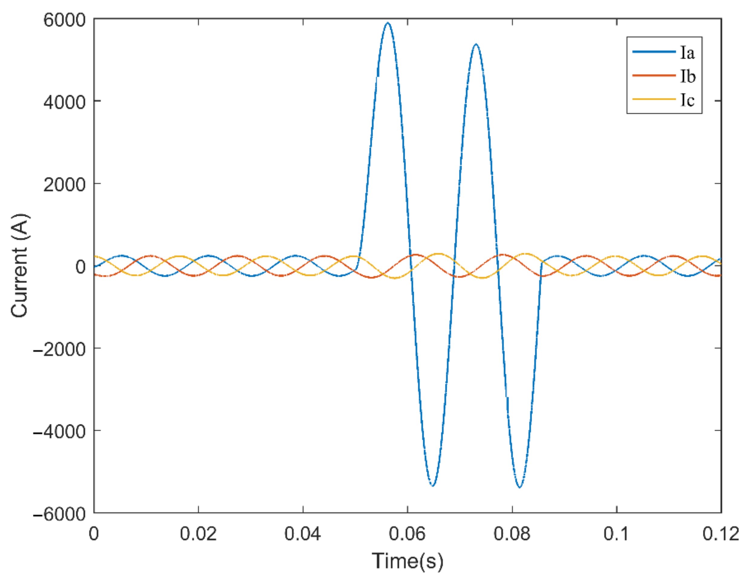
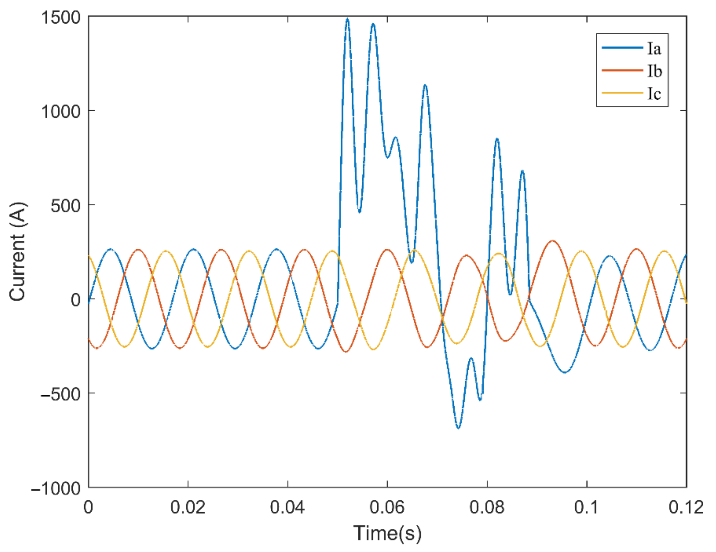
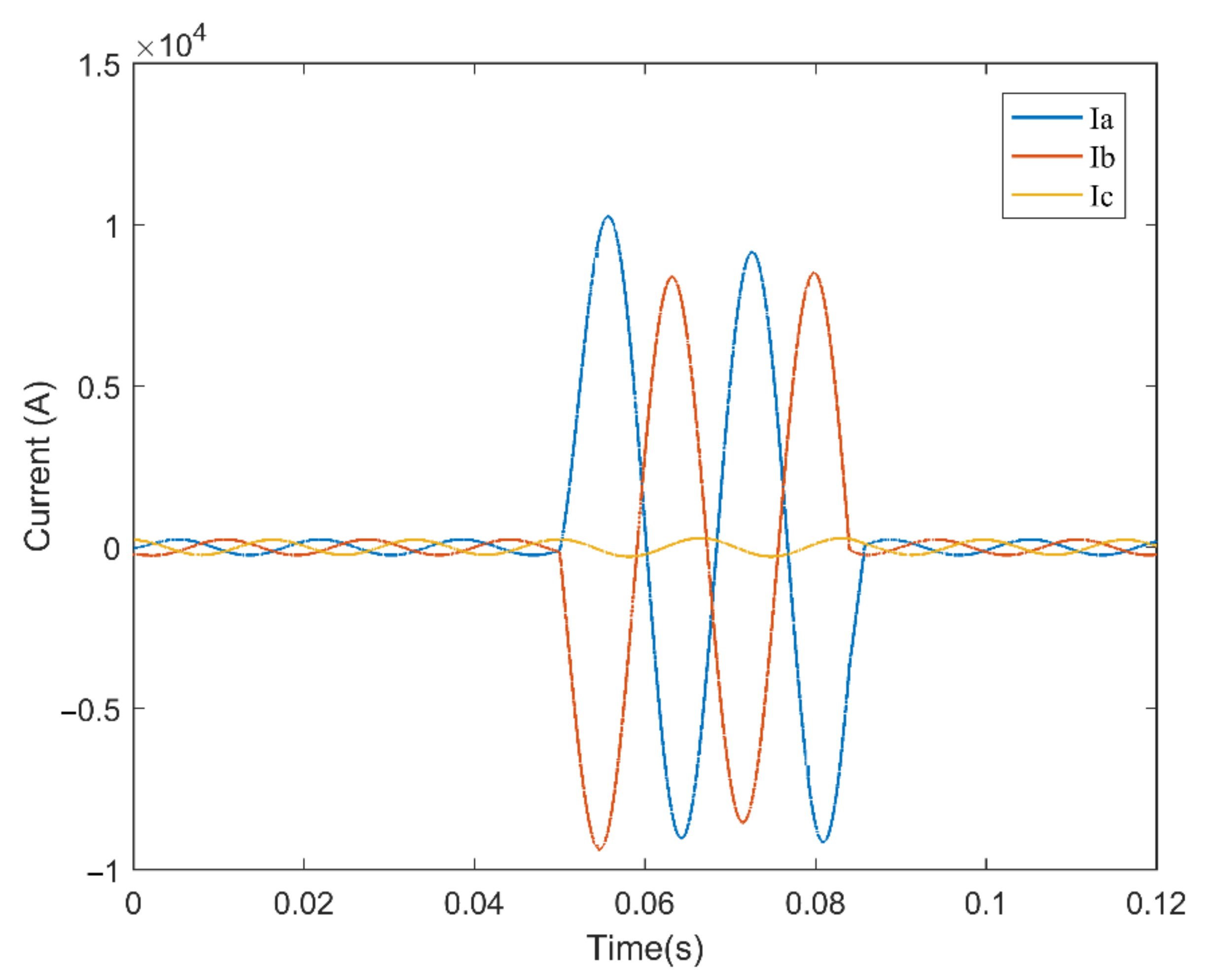
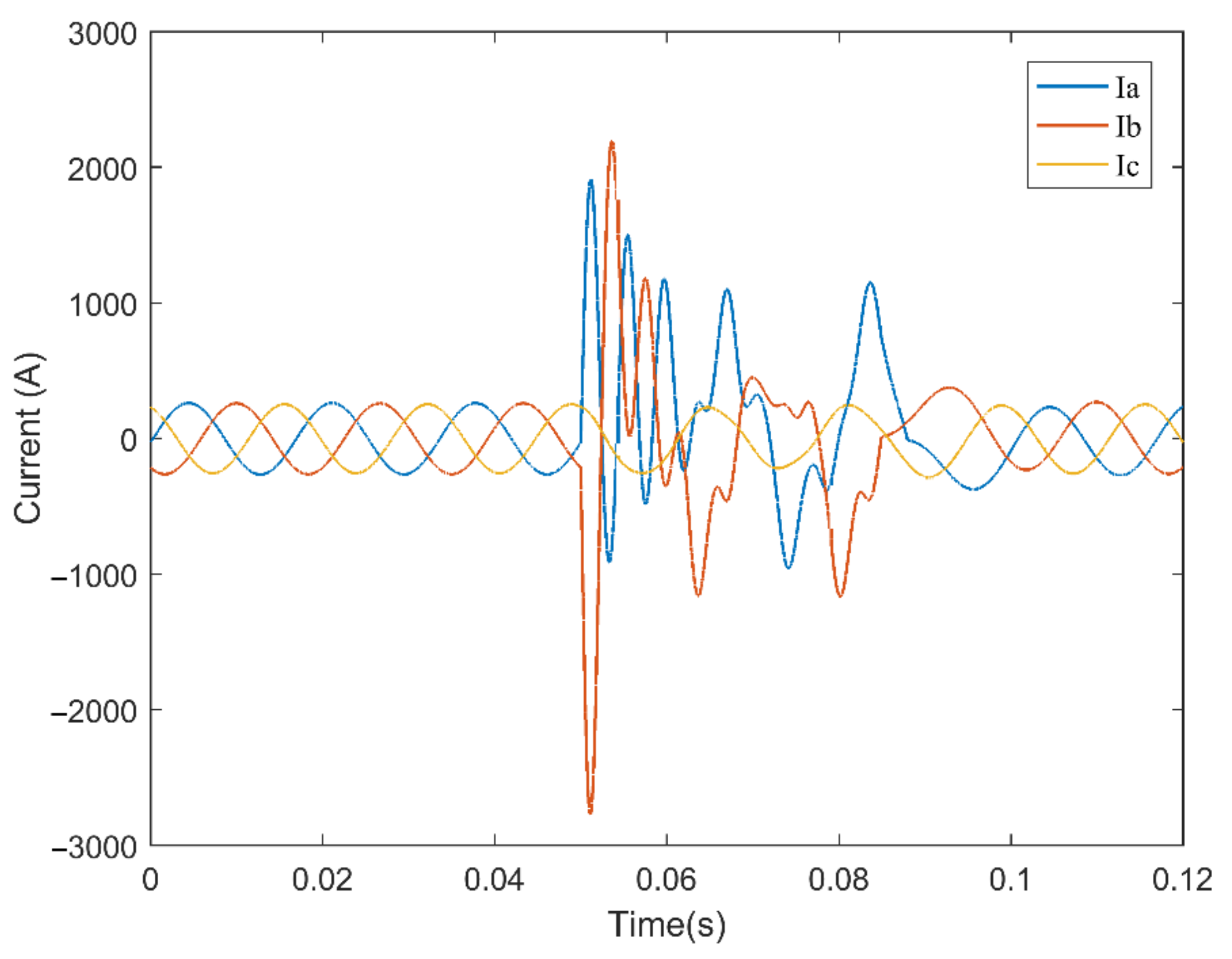
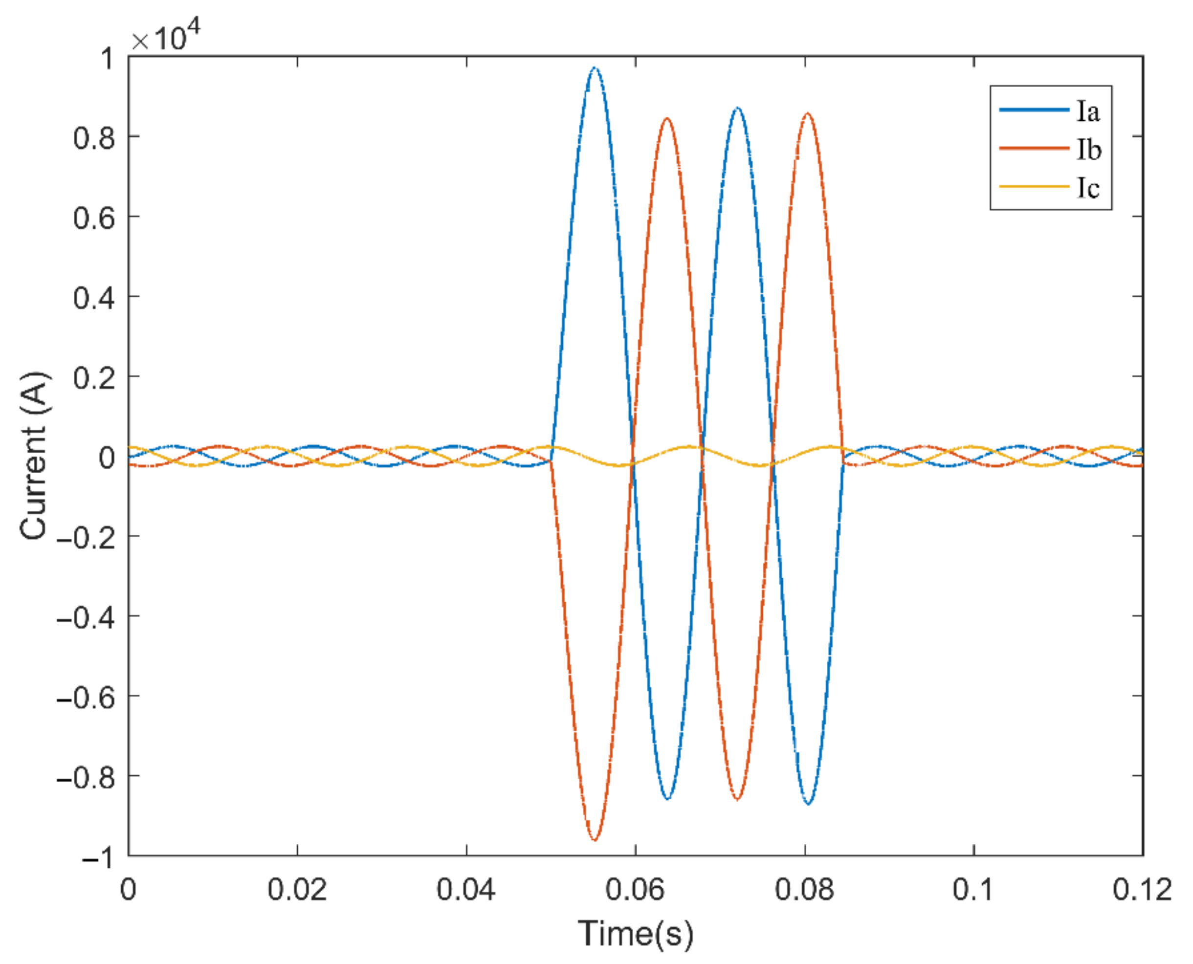
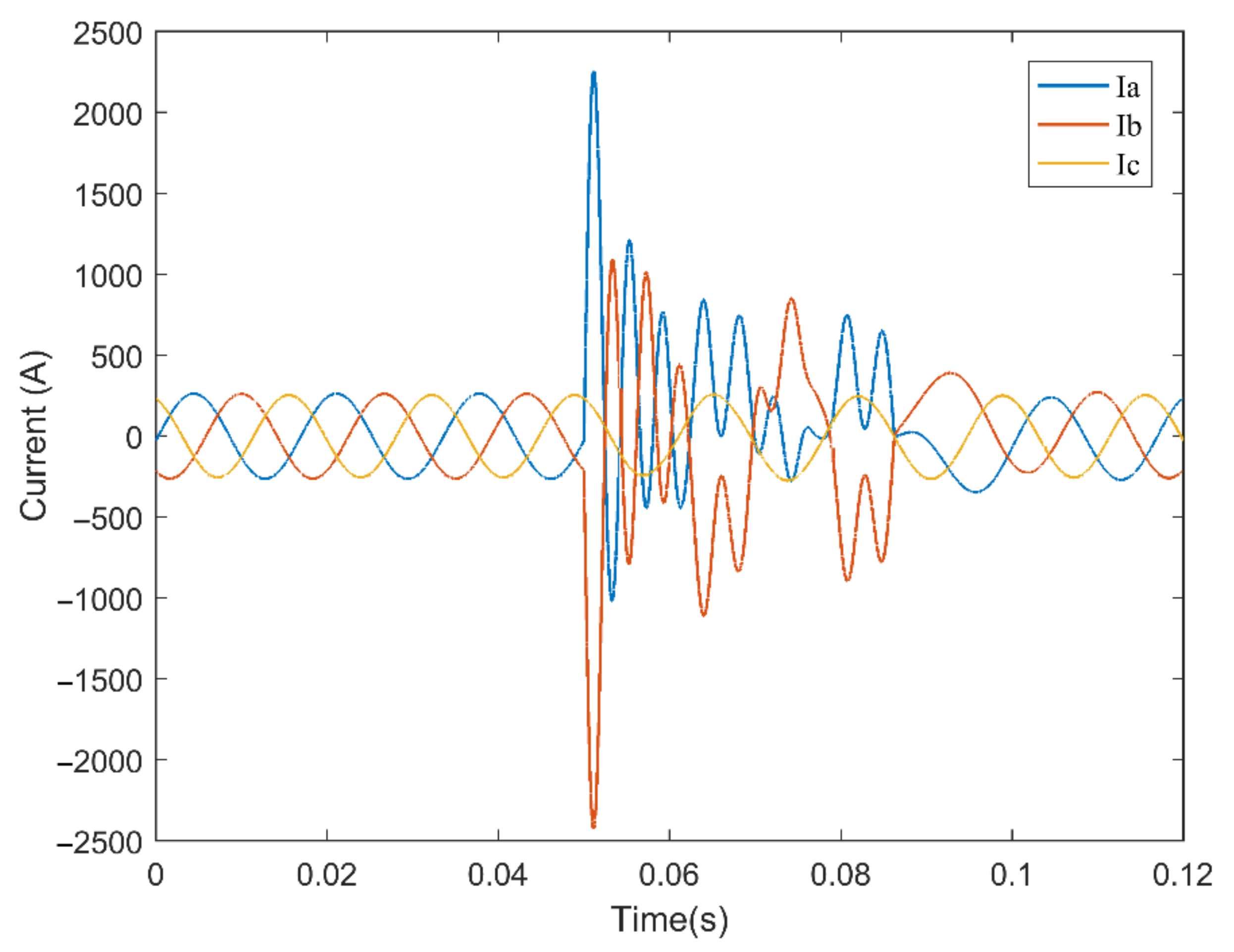
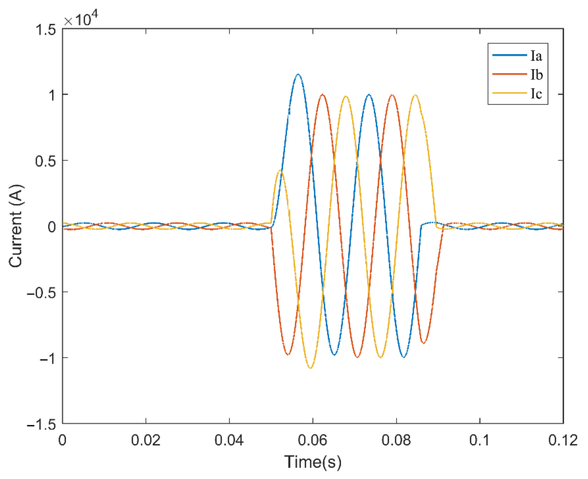
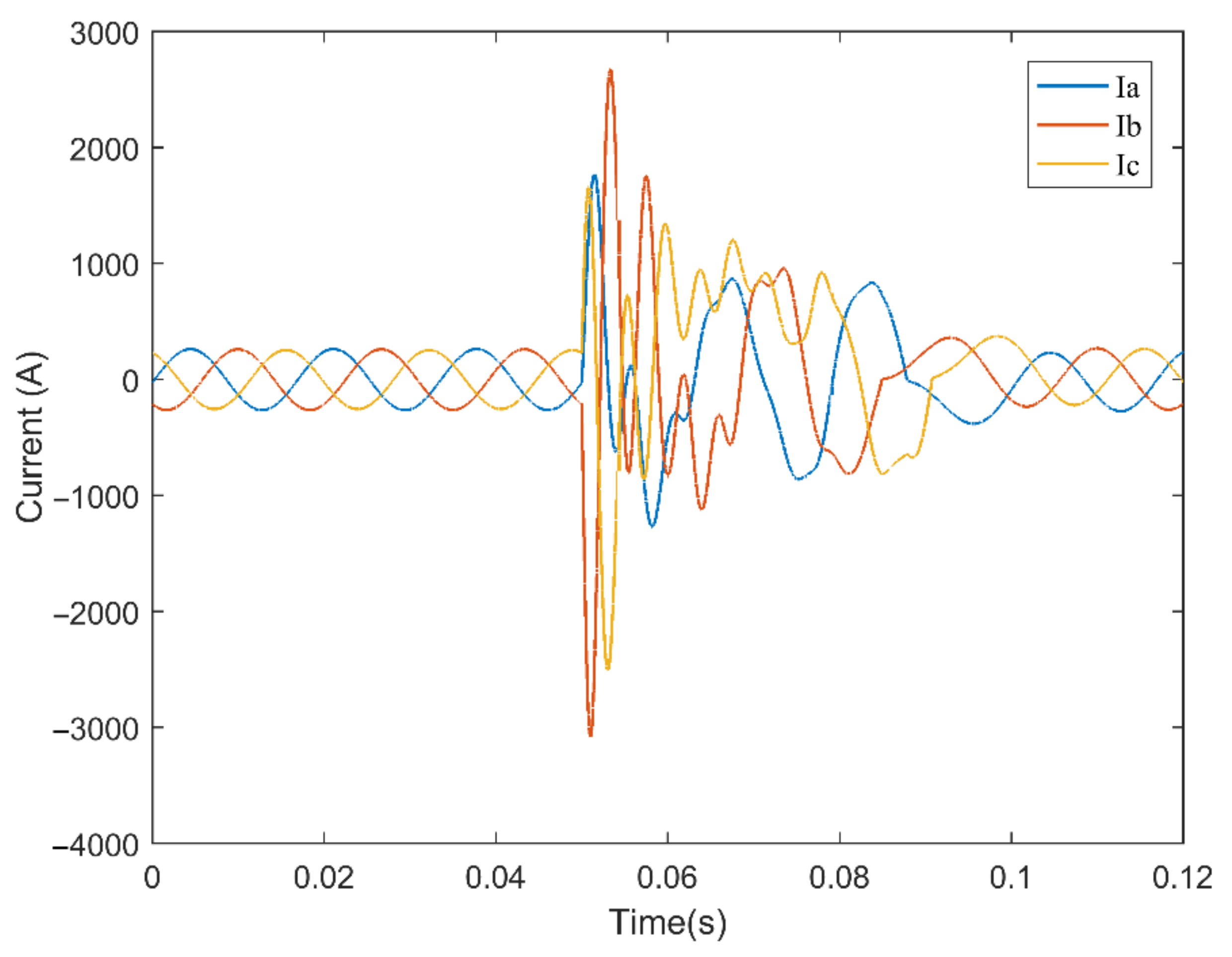
The presented results show that the fault detection technique based on monitoring the instantaneous current value and its first derivative can detect different fault situations in a distribution system. The fault detection speed was found to depend on the PSR used and the type of fault present in the electrical system. The SLG fault was detected more quickly in the abc reference, with PSR = 50 µs and an average detection time of 63 µs. For the 2LG fault, detection was fastest in the dq0 reference, with PSR = 10 µs and an average detection time of 40 µs. When the fault was 2L, detection occurred faster in the abc and dq0 references, with PSR = 50 µs and an average detection time of 50 µs. Finally, detection of the 3LG fault was faster in the dq0 reference, with PSR = 10 µs and an average detection time of 45 µs. Considering all fault situations analyzed and independent of the PSR used, the total average detection time was 49 µs.

Instantaneous information makes protection devices with time-domain sensing technology faster than phase-based devices. This means that the protection relays present in systems operating at 60 Hz typically act between 17 and 25 ms, and faults are cleared between 50 and 67 ms.

The results of this study indicate that the fault detection technique based on monitoring the instantaneous value of the current and its first derivative is an alternative that can contribute to the improvement of protection devices in the time domain, especially in increasing the speed of action of these devices.

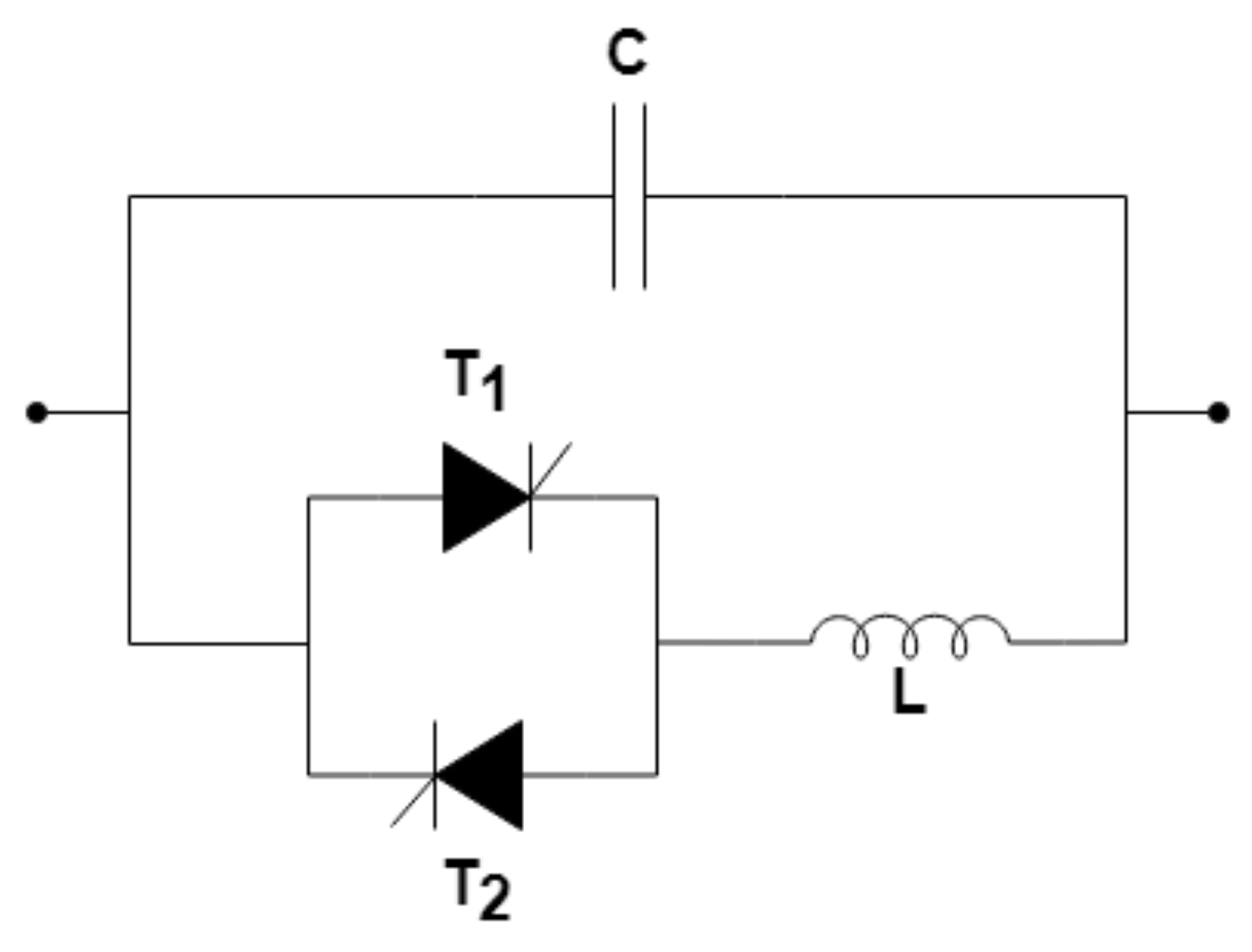
Regarding the limitation of fault currents, the detection technique associated with TCSC presented the expected behavior, causing the device to act as a variable impedance, limiting the fault current of the distribution system studied. Due to the potential growth in the number of DG units connected to traditional distribution systems, these systems tend to transform from radial unidirectional power flow networks to active networks in which the power flow can run in multiple directions and then, change the value of the short-circuit current. Considering that a TCSC is formed by controlled semiconductor switches and passive elements, its actuation time will basically depend on the fault detection time and the switching time of the switches, which is in the range from 5 to 400 µs.

According to the specialized literature, for systems operating at 60 Hz, actuation time of a recloser is typically less than 50 ms. Therefore, TCSC can be one of the alternatives to reduce the lack of coordination between the fuse and the recloser when temporary faults occur in distribution systems with DG.

7. Conclusions

The simplicity of implementation and the speed of fault detection, shown by the simulation results, indicate that the methodology presented in this paper can contribute to the improvement of protection devices that use current values in the time domain. The simultaneous monitoring of the current in three different references frames working together makes possible a faster fault detection in many situations. The complementary action of the references in the detection of the fault causes the activation of the protection device to be made by a control signal issued by the reference that detects the fault first.

The proposed methodology combined with the TCSC caused an average fault current reduction of approximately 70.56%, significantly contributing to the protection of the distribution system.

Future work will be directed at investigating the performance of the presented methodology in fault detection in medium-voltage distribution systems with the presence of microgrids, acting on the activation of SSFCL devices. This can be done through MATLAB/Simulink and tests performed in the hardware-in-the-loop (HIL) environment.

References

1. REN21. Renewables 2017 Global Status Report; REN21 Secretariat: Paris, France, 2017; ISBN 978-3-9818107-6-9. [Google Scholar]
2. Brearley, B.J.; Prabu, R.R. A review on issues and approaches for microgrid protection. Renew. Sustain. Energy Rev. 2017, 67, 988–997. [Google Scholar] [CrossRef]
3. Zeineldin, H.; Huchel, L. Planning the coordination of directional overcurrent relays for distribution systems considering DG. In Proceedings of the 2016 IEEE Power and Energy Society General Meeting (PESGM), Boston, MA, USA, 17–21 July 2016; Volume 7. pp. 1642–1649. [Google Scholar]
4. Sarwagya, K.; Nayak, P.K. An extensive review on the state-of-art on microgrid protection. In Proceedings of the 2015 IEEE Power, Communication and Information Technology Conference (PCITC), Odisha, India, 15–17 October 2015; pp. 862–866. [Google Scholar]
5. Udgave, A.D.; Jadhav, H. A review on Distribution Network protection with penetration of Distributed Generation. In Proceedings of the 2015 IEEE 9th International Conference on Intelligent Systems and Control (ISCO), Coimbatore, India, 9–10 January 2015; pp. 1–4. [Google Scholar]
6. Hosseini, S.A.; Abyaneh, H.A.; Sadeghi, S.H.H.; Razavi, F.; Nasiri, A. An overview of microgrid protection methods and the factors involved. Renew. Sustain. Energy Rev. 2016, 64, 174–186. [Google Scholar] [CrossRef]
7. Ghaemi, S.; Abapour, M. Effect of Fault Current Limiter (FCL) on reliability and protection coordination of distribution system. In Proceedings of the 2016 24th Iranian Conference on Electrical Engineering (ICEE), Shiraz, Iran, 10–12 May 2016; pp. 726–731. [Google Scholar]
8. Shahriari, S.A.A.; Abapour, M.; Yazdian, A.; Haghifam, M.R. Minimizing the impact of distributed generation on distribution protection system by solid state fault current limiter. In Proceedings of the IEEE PES T&D 2010, Sao Paulo, Brazil, 8–10 November 2010; pp. 1–7. [Google Scholar]
9. Alsalemi, S.; Almadhoun, S.; Najad, M.; Massoud, A.M.; Soliman, R. Design of a controlled solid state device for fault current limitation and arc flash suppression. In Proceedings of the 2017 IEEE Symposium on Computer Applications & Industrial Electronics (ISCAIE), Langkawi, Malaysia, 24–25 April 2017; pp. 48–53. [Google Scholar]
10. Fernandez, E.; Conde, A. Dynamic Analysis of Fault Current Limiters Performance in Distribution Systems. IEEE Lat. Am. Trans. 2016, 14, 171–178. [Google Scholar] [CrossRef]
11. Schmitt, H. Application and feasibility of fault current limiters in power systems; Cigré Work Group: Paris, France, 2012; Volume A3, p. 23. ISBN 978-2-85873-189-3. Available online: https://e-cigre.org/publication/497-application-and-feasibility-of-fault-current-limiters-in-power-systems (accessed on 3 October 2021).
12. Lu, X.; Wang, J.; Guerrero, J.M.; Zhao, D. Virtual-Impedance-Based Fault Current Limiters for Inverter Dominated AC Microgrids. IEEE Trans. Smart Grid 2018, 9, 1599–1612. [Google Scholar] [CrossRef] [Green Version]
13. Radmanesh, H.; Fathi, S.; Gharehpetian, G. Thyristor-Controlled AC Reactor Based Fault Current Limiter for Distribution Network Stability Enhancement. J. Electr. Eng. Technol. 2016, 11, 1070–1076. [Google Scholar] [CrossRef] [Green Version]
14. Ueda, T.; Morita, M.; Arita, H.; Kida, Y.; Kurosawa, Y.; Yamagiwa, T. Solid-state current limiter for power distribution system. IEEE Trans. Power Deliv. 1993, 8, 1796–1801. [Google Scholar] [CrossRef]
15. Schweitzer, E.O.; Hou, D. Filtering for protective relays. In Proceedings of the IEEE WESCANEX 93 Communications, Computers and Power in the Modern Environment—Conference Proceedings, Saskatoon, SK, Canada, 17–18 May 1993; pp. 15–23. [Google Scholar]
16. Kasztenny, B.; Voloh, I.; Udren, E.A. Rebirth of the Phase Comparison Line Protection Principle. In Proceedings of the 59th Annual Conference for Protective Relay Engineers, College Station, TX, USA, 4–6 April 2006. [Google Scholar]
17. Campoccia, A.; Di Silvestre, M.L.; Incontrera, I.; Sanseverino, E.R.; Spoto, G. An efficient diagnostic technique for distribution systems based on under fault voltages and currents. Electr. Power Syst. Res. 2010, 80, 1205–1214. [Google Scholar] [CrossRef]
18. Dzienis, C.; Kereit, M.; Blumschein, J.; Claus, M. An experimental analysis of high-speed-distance protection. In Modern Electric Power Systems, Proceedings of the International Symposium on Modern Electric Power Systems (MEPS), Wroclaw, Poland, 20–22 September 2010; IEEE: Piscataway, NJ, USA, 2011. [Google Scholar]
19. Finney, D.; Zhang, Z.; Cardenas, J. Ultra fast distance protection. In Proceedings of the 10th IET International Conference on Developments in Power System Protection (DPSP 2010), Manchester, UK, 29 March–1 April 2010. [Google Scholar]
20. Schweitzer, E.O.; Kasztenny, B.; Guzman, A.; Skendzic, V.; Mynam, M.V. Speed of line protection—Can we break free of phasor limitations? In Proceedings of the 41st Annual Western Conference for Protective Relay Engineers, Spokane, WA, USA, 14–16 October 2014; pp. 448–461. [Google Scholar]
21. Schweitzer, E.O.; Kasztenny, B.; Mynam, M.V. Performance of time-domain line protection elements on real-world faults. In Proceedings of the 2016 69th Annual Conference for Protective Relay Engineers (CPRE), College Station, TX, USA, 4–7 April 2016; pp. 1–17, ISSN 2474-9753. [Google Scholar]
22. Kasztenny, B.; Guzmán, A.; Fischer, N.; Mynam, M.V.; Taylor, D. Practical setting considerations for protective relays that use incremental quantities and traveling waves. In Proceedings of the 43rd Annual Western Protective Relay Conference, Washington, DC, USA, 18–20 October 2016. [Google Scholar]
23. Guzmán, A.; Mynam, M.; Skendzic, V.; Eternod, J.L. Directional elements—How fast can they be. In Proceedings of the 44th Annual Western Protective Relay Conference, Spokane, WA, USA, 17–19 October 2017. [Google Scholar]
24. Sharma, S.; Kathe, A.; Joshi, T.; Kanagasabai, T. Application of Ultra-High-Speed Protection and Traveling-Wave Fault Locating on a Hybrid Line. In Proceedings of the 46th Annual Western Protective Relay Conference, Spokane, WA, USA, 21–24 October 2019. [Google Scholar]
25. Mohammadi, F.; Nazri, G.-A.; Saif, M. A Fast Fault Detection and Identification Approach in Power Distribution Systems. In Proceedings of the 2019 International Conference on Power Generation Systems and Renewable Energy Technologies (PGSRET), Istanbul, Turkey, 26–27 August 2019; pp. 1–4. [Google Scholar]
26. Zhang, C.; Wang, J.; Huang, J.; Cao, P. Detection and classification of short-circuit faults in distribution networks based on Fortescue approach and Softmax regression. Int. J. Electr. Power Energy Syst. 2020, 118, 105812. [Google Scholar] [CrossRef]
27. Wang, A.; Wang, Y. Distribution System Fault Detection through Feature-Summarizing Matrix: A Case Study. In Proceedings of the 2020 IEEE Power & Energy Society General Meeting (PESGM), Virtual Event, 2–6 August 2020; pp. 1–5. [Google Scholar]
28. Liu, Z.; Hu, Z.; Li, Y.; Peng, H.; Zhu, L.; Mo, W. Fault Detection System for 500kV AC Fault Current Limiter Based on High-Coupled Split Reactor. In Proceedings of the 2020 IEEE International Conference on Applied Superconductivity and Electromagnetic Devices (ASEMD), Tianjin, China, 16–18 October 2020. [Google Scholar]
29. Abbas, A.S.; El-Sehiemy, R.A.; El-Ela, A.A.; Ali, E.S.; Mahmoud, K.; Lehtonen, M.; Darwish, M.M.F. Optimal Harmonic Mitigation in Distribution Systems with Inverter Based Distributed Generation. Appl. Sci. 2021, 11, 774. [Google Scholar] [CrossRef]
30. Lima, E.M.; Coelho, R.d.A.; Brito, N.S.D.; de Souza, B.A. High impedance fault detection method for distribution networks under non-linear conditions. Int. J. Electr. Power Energy Syst. 2021, 131, 107041. [Google Scholar] [CrossRef]
31. Li, X.; Dysko, A.; Burt, G. Traveling Wave-Based Protection Scheme for Inverter-Dominated Microgrid Using Mathematical Morphology. IEEE Trans. Smart Grid 2014, 5, 2211–2218. [Google Scholar] [CrossRef] [Green Version]
32. Gush, T.; Bukhari, S.B.A.; Haider, R.; Admasie, S.; Oh, Y.-S.; Cho, G.-J.; Kim, C.-H. Fault detection and location in a microgrid using mathematical morphology and recursive least square methods. Int. J. Electr. Power Energy Syst. 2018, 102, 324–331. [Google Scholar] [CrossRef]
33. Mishra, M.; Panigrahi, R.R.; Rout, P.K. A combined mathematical morphology and extreme learning machine techniques based approach to micro-grid protection. Ain Shams Eng. J. 2019, 10, 307–318. [Google Scholar] [CrossRef]
34. Gururani, A.; Mohanty, S.R.; Mohanta, J.C. Microgrid protection using Hilbert–Huang transform based-differential scheme. IET Gener. Transm. Distrib. 2016, 10, 3707–3716. [Google Scholar] [CrossRef]
35. Chen, K.; Huang, C.; He, J. Fault detection, classification and location for transmission lines and distribution systems: A review on the methods. High Volt. 2016, 1, 25–33. [Google Scholar] [CrossRef]
36. Dehghani, M.; Khooban, M.H.; Niknam, T. Fast fault detection and classification based on a combination of wavelet singular entropy theory and fuzzy logic in distribution lines in the presence of distributed generations. Int. J. Electr. Power Energy Syst. 2016, 78, 455–462. [Google Scholar] [CrossRef]
37. Abdelgayed, T.S.; Morsi, W.G.; Sidhu, T.S. Fault Detection and Classification Based on Co-training of Semisupervised Machine Learning. IEEE Trans. Ind. Electron. 2018, 65, 1595–1605. [Google Scholar] [CrossRef]
38. Kar, S.; Samantaray, S.R. A Fuzzy Rule Base Approach for Intelligent Protection of Microgrids. Electr. Power Components Syst. 2015, 43, 2082–2093. [Google Scholar] [CrossRef]
39. Kar, S.; Samantaray, S.R. Time-frequency transform-based differential scheme for microgrid protection. IET Gener. Transm. Distrib. 2014, 8, 310–320. [Google Scholar] [CrossRef]
40. Kumar, D.S.; Srinivasan, D.; Reindl, T. A Fast and Scalable Protection Scheme for Distribution Networks with Distributed Generation. IEEE Trans. Power Deliv. 2016, 31, 67–75. [Google Scholar] [CrossRef]
41. Chaitanya, B.K.; Soni, A.K.; Yadav, A. Communication assisted fuzzy based adaptive protective relaying scheme for microgrid. J. Power Technol. 2018, 98, 57. [Google Scholar]
42. Thattai, K.; Sahoo, A.; Ravishankar, J. On-line and off-line fault detection techniques for inverter based islanded microgrid. In Proceedings of the 2018 IEEE 12th International Conference on Compatibility, Power Electronics and Power Engineering (CPE-POWERENG 2018), Doha, Qatar, 10–12 April 2018; pp. 1–6. [Google Scholar]
43. Escudero, R.; Noel, J.; Elizondo, J.; Kirtley, J. Microgrid fault detection based on wavelet transformation and Park’s vector approach. Electr. Power Syst. Res. 2017, 152, 401–410. [Google Scholar] [CrossRef]
44. Eslami, R.; Sadeghi, S.H.H.; Askarian-Abyaneh, H.; Nasiri, A. A Novel Method for Fault Detection in Future Renewable Electric Energy Delivery and Management Microgrids, Considering Uncertainties in Network Topology. Electr. Power Components Syst. 2017, 45, 1118–1129. [Google Scholar] [CrossRef]
45. Hussain, N.; Nasir, M.; Vasquez, J.C.; Guerrero, J.M. Recent Developments and Challenges on AC Microgrids Fault Detection and Protection Systems–A Review. Energies 2020, 13, 2149. [Google Scholar] [CrossRef]
46. Bellan, D. Clarke Transformation Solution of Asymmetrical Transients in Three-Phase Circuits. Energies 2020, 13, 5231. [Google Scholar] [CrossRef]
47. Duesterhoeft, W.C.; Schulz, M.W.; Clarke, E. Determination of Instantaneous Currents and Voltages by Means of Alpha, Beta, and Zero Components. Trans. Am. Inst. Electr. Eng. 1951, 70, 1248–1255. [Google Scholar] [CrossRef]
48. Park, R.H. Two-reaction theory of synchronous machines generalized method of analysis-part I. Trans. Am. Inst. Electr. Eng. 1929, 48, 716–727. [Google Scholar] [CrossRef]
49. Kreyzig, E. Advanced Engineering Mathematics; John Wiley and Sons: Hoboken, NJ, USA, 1999. [Google Scholar]
50. Moraes, I.J. Aplicação de TCSC na distribuição primária: Estudo de caso. Master’s Thesis, Federal University of Espírito Santo State, Vitoria, Brazil, 2016. [Google Scholar]
51. Hingorani, N.G.; Gyugyi, L. Understanding FACTS: Concepts and Technology of Flexible AC Transmission Systems; John Wiley & Sons, Inc.: Hoboken, NJ, USA, 2000. [Google Scholar]
Figure 1. Logic flowchart of the fault detector.
Energies 15 00526 g001
Figure 2. Single-line diagram of the distribution feeder.
Energies 15 00526 g002
Figure 3. Single-phase representation of TCSC.
Energies 15 00526 g003
Figure 4. Normal operation condition.
Energies 15 00526 g004
Figure 5. SLG fault with RF = 0 Ω.
Energies 15 00526 g005
Figure 6. Actuation of TCSC in limiting the current in SLG fault with RF = 0 Ω.
Energies 15 00526 g006
Figure 7. 2LG fault with RF = 0 Ω.
Energies 15 00526 g007
Figure 8. Actuation of TCSC in limiting the current in 2LG fault with RF = 0 Ω.
Energies 15 00526 g008
Figure 9. A 2L fault with RF = 0 Ω.
Energies 15 00526 g009
Figure 10. Actuation of TCSC in limiting the fault current in 2L with RF = 0 Ω.
Energies 15 00526 g010
Figure 11. A 3LG fault with RF = 0 Ω.
Energies 15 00526 g011
Figure 12. Actuation of TCSC in limiting the fault current in 3LG fault with RF = 0 Ω.
Energies 15 00526 g012