VMD-WSLSTM Load Prediction Model Based on Shapley Values

Abstract

Accurate short-term load forecasting can ensure the safe operation of the grid. Decomposing load data into smooth components by decomposition algorithms is a common approach to address data volatility. However, each component of the decomposition must be modeled separately for prediction, which leads to overly complex models. To solve this problem, a VMD-WSLSTM load prediction model based on Shapley values is proposed in this paper. First, the Shapley value is used to select the optimal set of special features, and then the VMD decomposition method is used to decompose the original load into several smooth components. Finally, WSLSTM is used to predict each component. Unlike the traditional LSTM model, WSLSTM can simplify the prediction model and extract common features among the components by sharing the parameters among the components. In order to verify the effectiveness of the proposed model, several control groups were used for experiments. The results show that the proposed method has higher prediction accuracy and training speed compared with traditional prediction methods.

1. Introduction

With the continuous progress of social science and technology, the application of electric power is becoming increasingly extensive, and there are more and more factors affecting the electric load, which leads to the non-smoothness and complexity of the electric load. Accurate prediction of power load data is beneficial to the relevant departments for policy making and power dispatching, and it is of great significance to the development of power systems. Therefore, determining how to accurately forecast the power load is a topic worthy of study.

Prediction by artificial intelligence algorithms is a current research hotspot in the field of load prediction, and artificial intelligence algorithms are more suitable for nonlinear data, such as random forests [1,2], artificial neural networks [3,4], and support vector machines [5]. Among them, long short-term memory (LSTM) network is optimized on the basis of RNN. LSTM has a unique gate structure design that effectively overcomes the problem of gradient explosion or disappearance in RNN; it can effectively explore the intrinsic relationship between temporal data and has better accuracy when processing temporal data compared with other intelligent algorithms [6]. Currently, LSTM is studied and applied in many fields, such as load prediction [7], action recognition [8], and speech recognition [9].

However, with the continuous intensification of research, people have found that it is difficult to obtain ideal results using only a single algorithm, and a single algorithm generally has disadvantages such as slow calculation speed and large resource consumption [10]. Based on this, combined prediction methods have been proposed, of which load decomposition plus prediction is among the better ideas.

Zhu et al. [11] used EMD-Fbprophet-LSTM to predict the daily electricity consumption of enterprises to address the nonstationary nature of electricity consumption data. Semero et al. [12] used empirical modal decomposition (EMD) to decompose the short-term load in a microgrid to obtain better prediction results. Although EMD can reduce the randomness and volatility of the data, it is recursive in nature, and modal confusion occurs when intermittent signals are present in the original signal. Later, based on EMD, ensemble empirical modal decomposition (EEMD) was established by adding white noise to the original signal, and this modification can avoid the phenomenon of modal confusion in the decomposition process. Tang et al. [13] combined ensemble empirical modal decomposition (EEMD) with a deep belief network (DBN) and a bidirectional recurrent neural network (BIRNN) to establish the EEMD-DBN-BIRNN electric load model.

Azam et al. [14] combined ensemble empirical modal decomposition (EEMD) with a bidirectional long short-term memory network (BiLSTM) to obtain more accurate results for forecasting the electricity load one day ahead. Although EEMD can solve the modal mixing phenomenon in EMD, it adds white noise to the original signal, which can contaminate the fluctuation trend of the original signal. Variable modal decomposition (VMD) can choose the number of modal components after decomposition according to the actual situation, and it adopts a nonrecursive processing strategy to decompose the original signal by constructing and solving the constrained variational problem, which has the advantages of better signal decomposition accuracy and anti-interference. At present, VMD is widely used in power load forecasting [15,16,17], wind speed forecasting [18,19], energy price forecasting [20], etc. Although the decomposition algorithm to decompose the original load is helpful to reduce the non-smoothness of the data and thus improve the accuracy of the model, it requires each component of the decomposition to be modeled separately for prediction, which not only makes the model computationally intensive and the training time longer but also makes the extraction of common features among each component inadequate.

The accuracy of load forecasting generally depends on two major aspects: the forecasting method and feature processing. The forecasting method is continuously optimized, while feature processing is also studied in depth. Feature processing generally refers to the analysis of various features affecting the load to identify the features that have a greater impact on the load, after which the optimal set of features is selected, which reduces interference by features that have a smaller impact on the load in the model. Previous studies [13,21] used the Pearson correlation coefficient (PCC) to analyze the correlation between power data and features, and several features with greater correlation with the load were selected as the input feature set to realize dimensionality reduction and the selection of data. Ge et al. [22] quantified the correlation between load and input features using the maximum information criterion (MIC) and used FA to filter the features and eliminate invalid features. The above methods mainly use a number of features with a high correlation with the load data as input features; however, the feature-to-feature redundancy is not taken into account. In order to solve the problem of redundancy, people started to use the maximum correlation minimum redundancy [23,24] (mRMR) algorithm to select the optimal feature set based on the principle of maximizing the correlation between the feature set and the load data while minimizing the redundancy between the features and using incremental search to select the features.

Most of the existing methods use only linear analysis methods to analyze features, but there is a complex, nonlinear relationship between features and load data, so such methods still have major limitations. The Shapley value [25] is a method in cooperative game theory that distributes benefits fairly to each member of a team based on the contribution of the members to the total benefit. Shapley values have been used in feature selection [26,27]. If each power impact factor is abstracted as a team member and the result of load forecasting is taken as the total benefit, the result of each feature for load impact forecasting can be measured by the Shapley value, and since Shapley is interpretable and can reflect the contribution of each feature, it is more able to reflect the nonlinear relationship between features and load compared to the traditional linear analysis method [26]. Based on the above related research, this paper proposes a VMD-WSLSTM load prediction model based on Shapley values. First, Shapley values are used for feature selection. Then, VMD is used to decompose the load data into several smooth components, and finally, the WSLSTM prediction model is constructed to predict the components.

Table 1. Comparison between the proposed method and traditional methods.

Literature Related to Prediction Methods			Literature Related to Feature Analysis
Methods	Principles	Authors	Methods	Principles	Authors
EMD LSTM Fbprophet	Each component is modeled separately	Zhu et al. [11]	PCC	Linear correlation	Tang et al. [13]
EEMD BiLSTM	Each component is modeled separately	Azam et al. [14]	MIC	Linear correlation	Jung et al. [22]
EEMD DBN	Each component is modeled separately	Tang et al. [13]	mRMR	Linear correlation	Ge et al. [23]
VMD WSLSTM	Intercomponent coefficient sharing	this paper	Shapley	Nonlinear contribution	This paper

shows the differences between the conventional load forecasting methods and the forecasting methods proposed in this paper. The innovation and contribution of this paper lie in the following aspects:

(1)

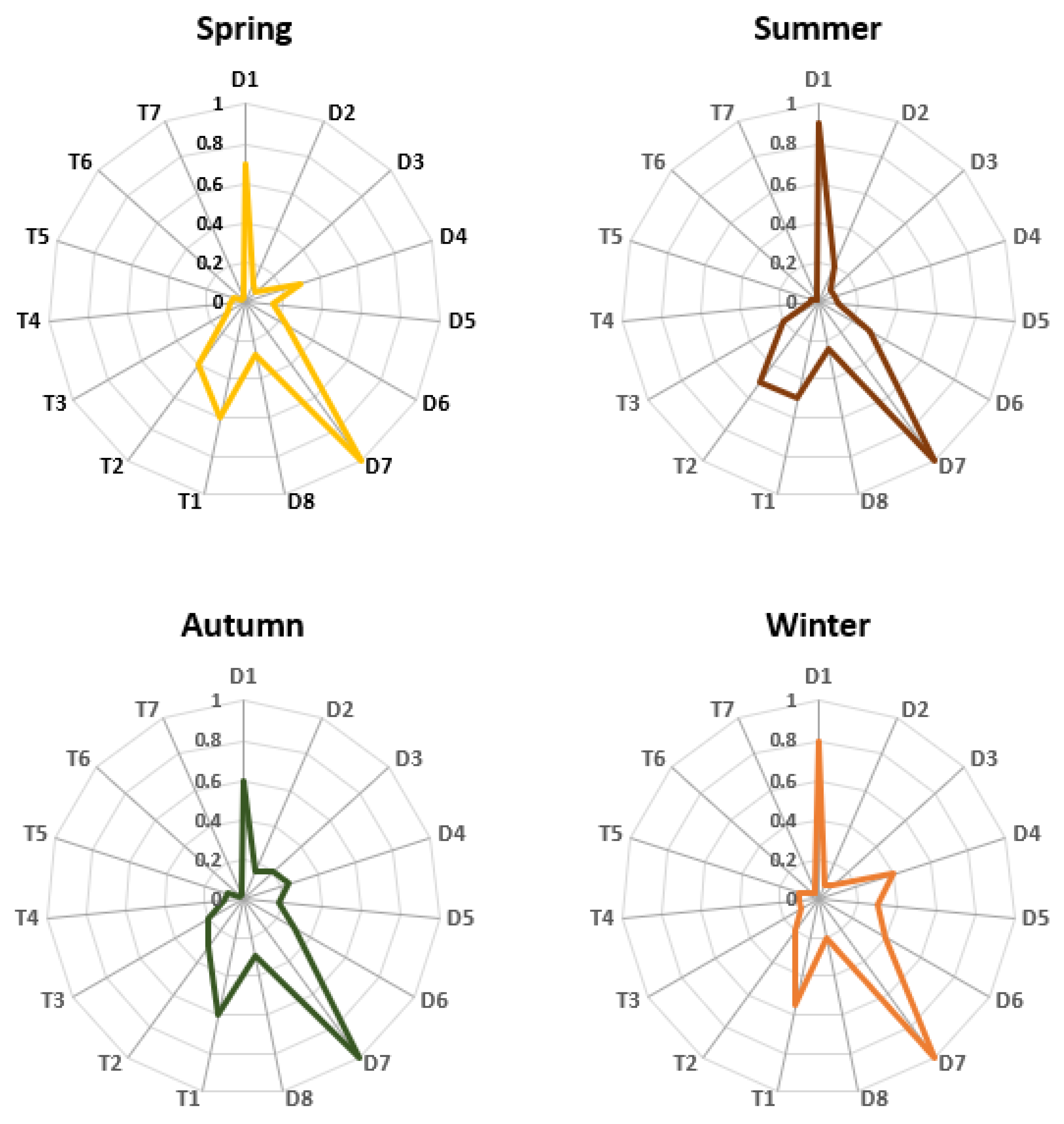
Considering the complex nonlinear relationship between the electric load and the features, we use the Shapley value for feature selection.

(2)

Considering the non-smoothness of the electric load, we use VMD to decompose the electric load and reduce the non-smoothness of the load.

(3)

Considering that the traditional load forecasting model based on the combination of decomposition and prediction will lead to too many model parameters and overly complicated training, we introduce the idea of weight sharing to LSTM and construct the WSLSTM model.

2. Materials and Methods

In this section, firstly, the feature selection method used in this paper is introduced, and the specific process and formulas are described in Section 2.1. Secondly, the VMD decomposition model is introduced, and the specific process and formulas are described in Section 2.2. Finally, the main prediction model, the WSLSTM model, is introduced, and the specific process and formulas are described in Section 2.3.

2.1. Feature Selection

In load forecasting studies, there are many factors that affect load fluctuations, and the relationship between factors and the load is highly complex and nonlinear. The Shapley value can effectively quantify the nonlinear relationship between features and the load [28]. The Shapley value is essentially a measure of marginal contribution. Based on this concept, the contribution of each feature to the load can be expressed by the Shapley value, and the average value of the marginal contribution of the jth feature of each n-dimensional sample in different feature subsets is the Shapley value of the feature. Its calculation formula is as follows.

$${\mathsf{\varphi }}_{\mathrm{j}}={\displaystyle \sum _S\frac{\left|\mathrm{s}\right|!(n-\left|\mathrm{s}\right|-1)!}{n!}(F_x(S\cup \{x^j\})-F_x(S))}$$

(1)

where ${\mathsf{\varphi }}_{\mathrm{j}}$ is the Shapley value of the jth feature in sample x, S is the subset of features not included in $x^j$, $\left|\mathrm{s}\right|$ is the number of features included in S, and $F_x(S)$ is the prediction result based on the set of S features.

From the formula, we know that to calculate the Shapley value of $x^j$, we need to calculate all combinations of features with and without $x^j$, and when the number of features is N, the combination of features to be considered is $2^N$. Obviously, when the number of features to be considered is large, it will lead to an exponential increase in computation. Therefore, in this paper, the Shapley value of the features is estimated using the Monte Carlo sampling method [29]. It is assumed that the input set of the model is $D={\{x_i,y_i\}}_{i=1}^n$, and the samples to be computed are denoted by $x_i$.

Step 1: Set the number of samples to M and reset the initial iterations to m = 1.

Step 2: Realign the features in $x_i$ to obtain a new alignment $x_{i,m}$.

$$x_{i,m}=\{x_i^{\left(1\right)},x_i^{\left(2\right)},\cdots ,x_i^{\left(j\right)},\cdots ,x_i^{\left(n\right)}\}$$

(2)

where n is the number of features in $x_{i,m}$, and $x_i^{\left(j\right)}$ is the jth feature in $x_{i,m}$.

Step 3: Sort the features in the selected sample v according to the order of $x_{i,m}$, yielding $v_m$.

$$v_m=\{v_{}^{\left(1\right)},v_{}^{\left(2\right)},\cdots ,v_{}^{\left(j\right)},\cdots ,v_{}^{\left(n\right)}\}$$

(3)

where n is the number of features in $v_m$, and $v_{}^{\left(j\right)}$ denotes the jth feature in $v_m$.

Step 4: Construct two new samples from the aligned $x_{i,m}$ and $v_m$.

$$x_m^{+j}=\{x_i^{\left(1\right)},x_i^{\left(2\right)},\cdots ,x_i^{\left(j-1\right)},x_i^{\left(j\right)},v_{}^{\left(j+1\right)},\cdots ,v_{}^{\left(n-1\right)},v_{}^{\left(n\right)}\}$$

(4)

$$x_m^{-j}=\{x_i^{\left(1\right)},x_i^{\left(2\right)},\cdots ,x_i^{\left(j-1\right)},v_{}^{\left(j\right)},v_{}^{\left(j+1\right)},\cdots ,v_{}^{\left(n-1\right)},v_{}^{\left(n\right)}\}$$

(5)

Step 5: Input the two newly generated samples $x_{i,m}$ and $v_m$ into the trained GWO-LSTM prediction model to calculate the prediction results and further obtain the marginal contribution of feature $x_i^{\left(j\right)}$ to the prediction results ${\mathsf{\varphi }}_{{}_{i,m}}^{\left(j\right)}$.

$${\mathsf{\varphi }}_{{}_{i,m}}^{\left(j\right)}=\stackrel{\wedge }{F}\left(x_m^{+j}\right)-\stackrel{\wedge }{F}\left(x_m^{-j}\right)$$

(6)

Step 6: Set m = m + 1 and loop through step (3) to step (8) until m > M when the loop stops.

Step 7: Calculate the average value of the marginal contribution of feature $x_i^{\left(j\right)}$ obtained in M cycles, which is the Shapley value of $x_i^{\left(j\right)}$.

$${\mathsf{\varphi }}_i^{\left(j\right)}=\frac{1}{M}{\displaystyle \sum _{m=1}^M{\mathsf{\varphi }}_{i,m}^{\left(j\right)}}$$

(7)

For dataset D, the average absolute value of the Shapley value $K_j$ of the feature in dataset D can be considered the Shapley value of the feature for the total load prediction result, which is calculated as:

$$K_j=\frac{1}{n}{\displaystyle \sum _{i=1}^n\left|{\mathsf{\varphi }}_i^{\left(j\right)}\right|}$$

(8)

The Shapley value measures the importance of a feature for the load, and the larger the Shapley value of a feature, the greater the impact on the load.

2.2. Variable Modal Decomposition

Variable modal decomposition [30] was proposed by Dragomiretskiy et al. on the basis of empirical modal decomposition. It is a nonrecursive, adaptive method for decomposing nonsmooth signals and is able to choose the number of modes for decomposition autonomously. The decomposed modal component (IMF) is a bandwidth-constrained amplitude modulation function with good noise robustness.

The VMD first calculates the analyzed signal for each modal component $u_k(t)$ by Hilbert transform to obtain the one-sided spectrum.

$$\left(\delta (t)+\frac{j}{\pi t}\right)u_k(t)$$

(9)

The signal resolved in each mode and its corresponding center frequency index $e^{-jwk}$ are mixed to shift the spectrum of each mode to the corresponding fundamental frequency band.

$$\left[\left(\delta (t)+\frac{j}{\pi t}\right)u_k(t)\right]e^{-jwk}$$

(10)

The gradient-squared L-parameter is calculated by demodulating the Gaussian smoothness of the signal and the gradient-squared criterion, from which the bandwidth of each modal signal is estimated with the variational constraint model as:

$$\underset{\left\{u_k\right\},\left\{w_k\right\}}{\min }\left\{{{\displaystyle \sum _k\Vert {\partial }_t\left[\left(\delta \left(t\right)+\frac{j}{\pi t}\right)\ast u_k\left(t\right)\right]e^{-j{w}_{k}t}\Vert }}_2^2\right\}$$

(11)

$$s.t.{\displaystyle \sum _{k=1}^k{u}_k}=f$$

(12)

where ${\partial }_{\mathrm{t}}$ is the Dirac function, $\left\{u_k\right\}$ is the decomposition of the modal components, $\left\{w_k\right\}$ is the corresponding central frequency of each modal component, and ∗ is the convolution operation.

Introducing the Lagrange multiplier operator λ(t) and the quadratic penalty factor α turns it into an unconstrained variational model.

$$\begin{array}{l}L\left(\left\{u_k\right\},\left\{w_k,\lambda \right\}\right)=\alpha {{\displaystyle \sum _k\Vert {\partial }_t\left[\left(\delta \left(t\right)+\frac{j}{\pi \mathrm{t}}\right)\ast u_k\left(t\right)\right]e^{-j{w}_{k}t}\Vert }}_2^2\\ +{\Vert f\left(t\right)-{\displaystyle \sum _k{u}_k\left(t\right)}\Vert }_2^2+\left[\lambda \left(t\right),f\left(t\right)-{\displaystyle \sum _k{u}_k\left(t\right)}\right]\end{array}$$

(13)

In order to obtain the optimal value of Equation (11), VMD applies the multiplicative operator alternation method to cyclically update each decomposition signal $\left\{u_k\right\}$ and its corresponding center frequency $\left\{w_k\right\}$ with the cyclic update of Equations (14) and (15).

$$u_k^{n+1}\left(w\right)=\frac{f\left(w\right)-{\displaystyle \sum _{i\ne k}{u}_i\left(w\right)}+\frac{u\left(w\right)}{2}}{1+2a{\left(w-w_k\right)}^2}$$

(14)

$$w_k^{n+1}=\frac{{\displaystyle {\int }_0^{\infty }\omega {\left|u_k\left(\omega \right)\right|}^{2}d\omega }}{{\displaystyle {\int }_0^{\infty }{\left|u_k\left(\omega \right)\right|}^{2}d\omega }}$$

(15)

when the loop iteration satisfies Equation (16), the loop terminates, and the final modal component is obtained as follows.

$${\displaystyle \sum _k\frac{{\Vert u_k^{n+1}-u_k^n\Vert }_2^2}{{\Vert u_k^n\Vert }_2^2}<\epsilon },n<N$$

(16)

2.3. WSLSTM

Long short-term memory networks [31] (LSTM) were first proposed in 1997. Compared with RNN, the LSTM model introduces the concepts of memory cells and gates, replaces the neurons in the traditional neural network with memory cells, and adds forget gates, input gates, and output gates. The LSTM structure is able to store more long-term information and remove the unimportant information, so it can process the temporal data efficiently. Figure 1 shows the basic structure of LSTM.

The calculation process is shown in Equations (17)–(22):

$$\begin{array}{c}{f}_t=\sigma \left(w_f\left[h_{t-1},x_t\right]+b_f\right)\end{array}$$

(17)

$$\begin{array}{c}{i}_t=\sigma \left(w_i\left[h_{t-1},x_t\right]+b_i\right)\end{array}$$

(18)

$$\begin{array}{c} g_t=tanth\left(w_c\left[h_{t-1},x_t\right]+b_c\right)\end{array}$$

(19)

$$\begin{array}{c}{C}_t=f_t\times C_{t-1}+i_t\times g_t\end{array}$$

(20)

$$\begin{array}{c} o_t=\sigma \left(w_o\left[h_{t-1},x_t\right]+b_o\right)\end{array}$$

(21)

$$\begin{array}{c}{h}_t=o_t\times tanth\left(C_t\right)\end{array}$$

(22)

First, we calculate the state of the forget gate $f_t$, which takes values from 0 to 1, and $f_t$ determines the extent to which the last moment of the model’s memory state $C_{t-1}$ is preserved. $h_{t-1}$ is the output of the previous moment, $x_t$ is the new input information, and $w_f$ is the weight matrix of the forget gate. After the model retains the relevant information from the memory state of the previous moment through the forget gate, it then determines the new information to be added through the input gate $i_t$.$w_i$ is the weight matrix of the input gates. $C_t$ is the updated memory cell state, and $g_t$ is the preparatory information to be input into $C_t$. Finally, the output of the current moment $h_t$ is calculated through the output gate $o_t$, b is the bias matrix, and tanh is the activation function.

The weight-sharing mechanism [32,33] (WS) is a new idea that has emerged in recent years and is involved in image recognition, language interaction, etc. WSLSTM applies the idea of weight sharing, the essence of which lies in reducing parameters, simplifying the model, and extracting common features by sharing part of the structure of multiple independent LSTMs. The structure is similar to the stacked LSTM network structure, with the difference that WSLSTM shares one layer of the network structure. Specifically, after the original data are decomposed by the decomposition algorithm to obtain n modal components, it enters the corresponding independent LSTM, which is responsible for extracting the intrinsic features of each component. Then, it enters the LSTM layer with shared weights, which is responsible for resolving the common features of the components. Finally, it enters the independent LSTM layer, which is responsible for the final correction of the data, and the final prediction results are obtained by reconstructing the prediction results of each component after the correction. The existence of shared weights reduces the parameters of the model and improves its training speed. Figure 2 shows the structure of WSLSTM.

The forward calculation of WSLSTM is similar to that of an ordinary multilayer LSTM, and the neuron update at moment t of the nth layer LSTM network is formulated as follows:

$$\left[\begin{array}{c}\begin{array}{c}\begin{array}{c}{i}_t^{\left(n\right)}\\ f_t^{\left(n\right)}\end{array}\\ o_t^{\left(n\right)}\end{array}\\ g_t^{\left(n\right)}\end{array}\right]=\left[\begin{array}{c}\begin{array}{c}\begin{array}{c}\sigma \\ \sigma \end{array}\\ \sigma \end{array}\\ \tanh \end{array}\right]\left[\begin{array}{c}\begin{array}{cc}{W}_{i,x}^{\left(n\right)}& W_{i,h}^{\left(n\right)}\end{array}\\ \begin{array}{cc}{W}_{f,x}^{\left(n\right)}& W_{f,h}^{\left(n\right)}\end{array}\\ \begin{array}{cc}{W}_{o,x}^{\left(n\right)}& W_{o,h}^{\left(n\right)}\end{array}\\ \begin{array}{cc}{W}_{g,x}^{\left(n\right)}& W_{g,h}^{\left(n\right)}\end{array}\end{array}\right]=\left[\begin{array}{c}{h}_t^{\left(n-1\right)}\\ h_{t-1}^{\left(n\right)}\end{array}\right]$$

(23)

WSLSTM backpropagation is similar to the ordinary neural network when updating the weights. Error backpropagation is used to calculate the error between the model output data and the original load data, and the loss is recorded as the sum of the errors of all outputs. The minimum error method is used to adjust the weights.

2.4. The Framework of the Proposed Model

Figure 3 is the framework of the proposed method. Firstly, feature selection is performed using Shapley values, then the load data are decomposed into several modal components using VMD, and the component data are input to the WSLSTM model for prediction. Finally, the predicted values of each component are superimposed to obtain the final predicted values.

3. Evaluation Indicators

In this study, the root-mean-square error (RMSE), mean absolute percentage error (MAPE), and mean absolute error (MAE) were used to estimate the accuracy of the forecast results. The specific formula is as follows:

$$MAE=\frac{{\displaystyle {\sum }_{t=1}^L(y_t-\stackrel{\wedge }{y_t}}{)}^2}{L}$$

(24)

$$MAPE=\frac{{\displaystyle {\sum }_{t=1}^L\frac{\left|(y_t-\stackrel{\wedge }{y_t})\right|}{y_t}}}{L}\times 100\%$$

(25)

$$MSE=\frac{{{\displaystyle {\sum }_{i=1}^L(y_t-\stackrel{\wedge }{y}}}_t)}{L}$$

(26)

where $\stackrel{\wedge }{y_t}$ is the prediction result of the model at time t, $y_t$ is the actual load data at time t, and L is the total number of load data.

4. Case Study

In this section, we first present the data used for the experiments. To verify the validity of the proposed model, four datasets were used for testing, and multiple models were used for comparative analysis.

4.1. Data Introduction

The data used in this study are from the 9th Electrical Mathematical Modeling Contest. The full-year data of 2016 were selected as the experimental dataset with a one-hour data collection interval and 8760 data points in total. The mean-fill method was used to fill in the missing data in the dataset. To be able to better evaluate the model, the data were divided into four datasets according to seasons. Throughout the year, electricity load is at the highest level in summer due to the widespread use of cooling equipment and at a higher level in winter due to the use of heating equipment. In the fall and spring, the electricity load is in the middle level due to the moderate temperature. The specific information of the dataset is shown in

Table 2. Statistical information table of load data after filling.

Seasons	Sum	Max	Median	Min	Mean	Std
Spring	2160	36,334	22,321	55,784	22,310	7788
Summer	2208	48,113	36,010	21,066	35,443	6704
Autumn	2184	46,546	30,558	14,699	30,399	7174
Winter	2208	51,127	32,638	16,245	32,788	8018

(statistical information table of load data after filling).

In this study, the experimental data were divided in the ratio of 9:1; the first 90% of each dataset is the training set, and the last 10% is the test set. Combined with Figure 4, it can be seen that the loads in the four seasons have roughly the same trend, with larger fluctuations in spring and winter and smaller fluctuations in summer and autumn.

4.2. Feature Selection

The initial feature set is shown in

Table 3. Initial feature information table.

Serial Number	Feature	Feature Description
D1	Temperature	°C
D2	Rainfall	mm
D3	Relative humidity	RH (%)
D4	Type of month	There are 12 months in a year (1~12)
D5	Type of week	There are 7 days in a week (1~7)
D6	Type of day	There are 31 days in a month (1~31)
D7	Type of hour	There are 24 h in a day (1~24)
D8	Type of working day	Working days (1); Rest days (0)
Ti (T1~T7)	Hourly load values for the last i hours	MW

. In this study, we broadly considered weather features (temperature, rainfall, relative humidity, etc.), date features (month, number of days of the week, first day of the month, first hour of the day, and whether it is a weekday or not), and load features (hourly load values for the past 23 h).

The Shapley value of each season’s gas load characteristics was calculated, the absolute value was taken, and normalization processing was performed. As shown in Figure 5, the order of importance of the characteristics is approximately the same for each season, with the ‘type of hour’ contributing the most to the electrical load. Temperature contributes the most to the load in summer, followed by winter.

Features with normalized Shapley values greater than or equal to 0.1 were selected separately for each training set. The final set of features selected for each season is shown in

Table 4. The final feature selection result of four datasets.

Season	Feature
Spring	D1, D2, D4, D5, D6, D7, D8, T1, T2, T3
Summer	D1, D2, D5, D6, D7, D8, T1, T2, T3
Autumn	D1, D2, D3, D4, D5, D6, D7, D8, T1, T2, T3, T4
Winter	D1, D3, D4, D5, D6, D7, D8, T1, T2, T3, T4, T5

.

4.3. Variational Mode Decomposition

The VMD algorithm is able to decompose the original data into a number of smooth components, the number of which needs to be set in advance. Too large a number of decompositions can cause modal mixing, while too small a number of decompositions can lead to inadequate decomposition. In this study, the optimal number of decompositions was determined by calculating the central frequency of each modal component after decomposition. The optimal number of decompositions K and the central frequency for each dataset are shown in

Table 5. Load decomposition component central frequency.

Season	K	Central Frequency
		IMF1	IMF2	IMF3	IMF4	IMF5	IMF6
Spring	6	1.58 × 10−5	0.0835	0.0198	0.0437	0.0219	0.0348
Summer	5	1.86 × 10−5	0.0919	0.0312	0.0273	0.0423
Autumn	5	1.79 × 10−5	0.0792	0.0466	0.0326	0.0274
Winter	6	1.68 × 10−5	0.0761	0.0483	0.0289	0.0379	0.0118

. When the number of decompositions of the four datasets is 6, 5, 5, and 6, respectively, the central frequencies of each decomposition mode are dissimilar, proving that decomposition is more adequate at this point.

4.4. Experimental Results and Discussion

The components obtained from the decomposition were fed into the WSLSTM model for prediction, and the final results were obtained after superposition. From Figure 6, it can be seen that the prediction results of the model have a good fit to the original load, and the prediction results and the actual data generally match.

In order to further demonstrate the effectiveness and accuracy of the model proposed in this paper, different control models were designed for comparative analysis using training time, RMSE, MAE, and MAPE as indicators.

Firstly, in order to verify the effectiveness of the feature selection method proposed in this paper, three models were used for controlled experiments: the first model takes all features as input (FF), the second model uses the Pearson correlation coefficient method to select those with high correlation as the optimal feature set (PF), and the third model uses the Shapley value for model feature selection (SF). For more rigorous experiments, all three models used the VMD-WSLSTM model as the prediction model. The experimental prediction results are shown in Figure 7 and

Table 6. Prediction results of different decomposition methods (the best results of each model are bolded).

	Model	Time (s)	RMSE	MAE	MAPE
Spring	FF	489.32	887.13	683.67	4.17
	PF	532.47	820.56	627.39	3.62
	SF	602.75	762.83	597.55	3.10
Summer	FF	493.54	750.43	634.57	2.58
	PF	529.39	712.56	604.12	2.14
	SF	606.19	677.48	572.53	1.71
Autumn	FF	418.18	830.55	704.31	2.89
	PF	524.27	800.35	680.24	2.47
	SF	607.38	784.89	638.08	2.29
Winter	FF	498.28	512.42	430.78	2.76
	PF	520.14	480.14	414.65	1.78
	SF	604.29	460.59	398.17	1.49

. In terms of time, the training time is the shortest for the FF model because it does not have to perform feature selection. In terms of accuracy, in the four training sets, the SF model shows different degrees of decrease in RMSE, MAE, and MAPE compared with the PF and FF models, demonstrating that feature selection using Shapley values has better prediction accuracy compared with traditional feature selection using correlation.

Secondly, in order to verify the effectiveness of the VMD decomposition algorithm, three models were used for controlled experiments. The three models are SLSTM (stacked LSTM with three layers), EMD-WSLSTM, and VMD-WSLSTM. For more rigorous experiments, all three models used the same features for input, and the prediction results are shown in

Table 7. Prediction results of different decomposition methods (the best results of each model are bolded).

	Model	Time (s)	RMSE	MAE	MAPE
Spring	SLSTM (SL)	124.32	984.31	712.32	5.19
	EMD-WSLSTM (EW)	688.32	873.23	630.32	3.78
	VMD-WSLSTM (VW)	602.75	762.83	597.55	3.10
Summer	SLSTM (SL)	134.59	794.31	742.12	3.89
	EMD-WSLSTM (EW)	574.21	738.43	689.12	2.47
	VMD-WSLSTM (VW)	606.19	677.48	572.53	1.71
Autumn	SLSTM (SL)	127.56	957.31	740.43	3.16
	EMD-WSLSTM (EW)	694.31	829.31	680.54	2.45
	VMD-WSLSTM (VW)	607.38	784.89	638.08	2.29
Winter	SLSTM (SL)	139.34	590.32	580.32	2.54
	EMD-WSLSTM (EW)	694.23	520.41	490.32	1.67
	VMD-WSLSTM (VW)	604.29	460.59	398.17	1.49

and Figure 8. In terms of time, SLSTM has the shortest training time because it does not need to decompose the load into several components and only needs to build a separate model. The training speed of EMD-WSLSTM is slightly slower than that of VMD-WSLSTM. In terms of accuracy, the prediction results of both EMD-WSLSTM and VMD-WSLSTM are better than those of SLSTM, which proves that decomposing the load through decomposition improves the results. The prediction results of VMD-WSLSTM are better than those of EMD-WSLSTM, which proves that VMD is better than EMD in load decomposition.

Finally, in order to verify the effectiveness of the WSLSTM model proposed in this paper, three models were used for controlled experiments. The three prediction models are VMD-LSTM, VMD-GRU, and VMD-WSLSTM. For more rigorous experiments, the same features were used as input for all three models, and the prediction results are shown in

Table 8. Forecast results of different forecasting methods (the best results of each model are bolded).

	Model	Time (s)	RMSE	MAE	MAPE
Spring	VMD-LSTM (VL)	823.21	870.34	623.32	3.48
	VMD-GRU (VG)	780.32	843.23	613.21	3.29
	VMD-WSLSTM (VW)	602.75	762.83	597.55	3.10
Summer	VMD-LSTM (VL)	815.32	742.31	643.21	2.49
	VMD-GRU (VG)	787.21	703.21	603.32	2.14
	VMD-WSLSTM (VW)	606.19	677.48	572.53	1.71
Autumn	VMD-LSTM (VL)	812.23	814.32	658.32	2.89
	VMD-GRU (VG)	756.12	804.32	647.32	2.41
	VMD-WSLSTM (VW)	607.38	784.89	638.08	2.29
Winter	VMD-LSTM (VL)	831.32	482.31	450.31	2.12
	VMD-GRU (VG)	779.23	470.12	432.12	1.67
	VMD-WSLSTM (VW)	604.29	460.59	398.17	1.49

and Figure 9. In terms of time, the training speed of VMD-LSTM is slightly slower than that of VMD-GRU because the structure of LSTM is more complicated than that of GRU. The training speed of VMD-WSLSTM is improved compared with that of VMD-LSTM and VMD-GRU, which proves that the model can be effectively simplified, and the training efficiency of the model can be improved by establishing a weight-sharing mechanism among the components. In terms of accuracy, the prediction results of VMD-WSLSTM are better than those of VMD-LSTM, which proves that extracting common features among components through the weight-sharing mechanism can not only improve the training speed of the model but also enhance its prediction accuracy.

To be able to further demonstrate the effectiveness of the proposed model, the model was compared with the existing GA-SVR, WD-LSSVM, CNN-LSTM, and VMD-LSSVM. The average values of the evaluation metrics are shown in

Table 9. Prediction results of different prediction models.

Models	RMSE	MAE	MAPE
GA-SVR	823.62	713.12	4.06
WD-LSSVM	780.14	694.31	3.65
CNN-LSTM	760.67	638.42	2.93
VMD-LSSVM	729.28	593.63	2.76
VMD-WSLSTM	605.15	551.58	2.15

and Figure 10. The RMSE of the prediction results of the proposed model is reduced by 218.47, 174.99, 155.52, and 124.13 compared with GA-SVR, WD-LSSVM, CNN-LSTM, and VMD-LSSVM, respectively. MAPE is reduced by 1.91%, 1.5%, 0.78%, and 0.61%, respectively. MAE is reduced by 161.54, 142.73, 86.84, and 42.05, respectively. This proves that the model proposed in this paper has better prediction accuracy than the traditional prediction model.

5. Conclusions

Accurate load forecasting can ensure the healthy operation of the power grid. In this paper, in order to improve the accuracy of the power load forecasting model, firstly, starting from the feature analysis, the Shapley value analysis method, which is different from the traditional feature analysis, is used to thoroughly explore the relationship between features and the load. Secondly, the idea of weight sharing is used to solve the problems of slow training and insufficient extraction of common features among components in the traditional model based on the combination of decomposition plus prediction. Controlled experiments using four datasets and multiple control groups led to the following conclusions:

(1)

Compared with the traditional method of feature selection using correlation, the Shapley value method proposed in this paper is more able to measure the importance of features to the load. The prediction accuracy of the model using Shapley values for feature selection is also improved compared with the traditional method.

(2)

The decomposition of the original load data using the decomposition algorithm can effectively reduce the complexity of the data, and the separate prediction of the decomposed components also helps to improve the prediction accuracy of the model. Compared with the EMD algorithm, the accuracy of the model decomposed by using the VMD algorithm is generally higher.

(3)

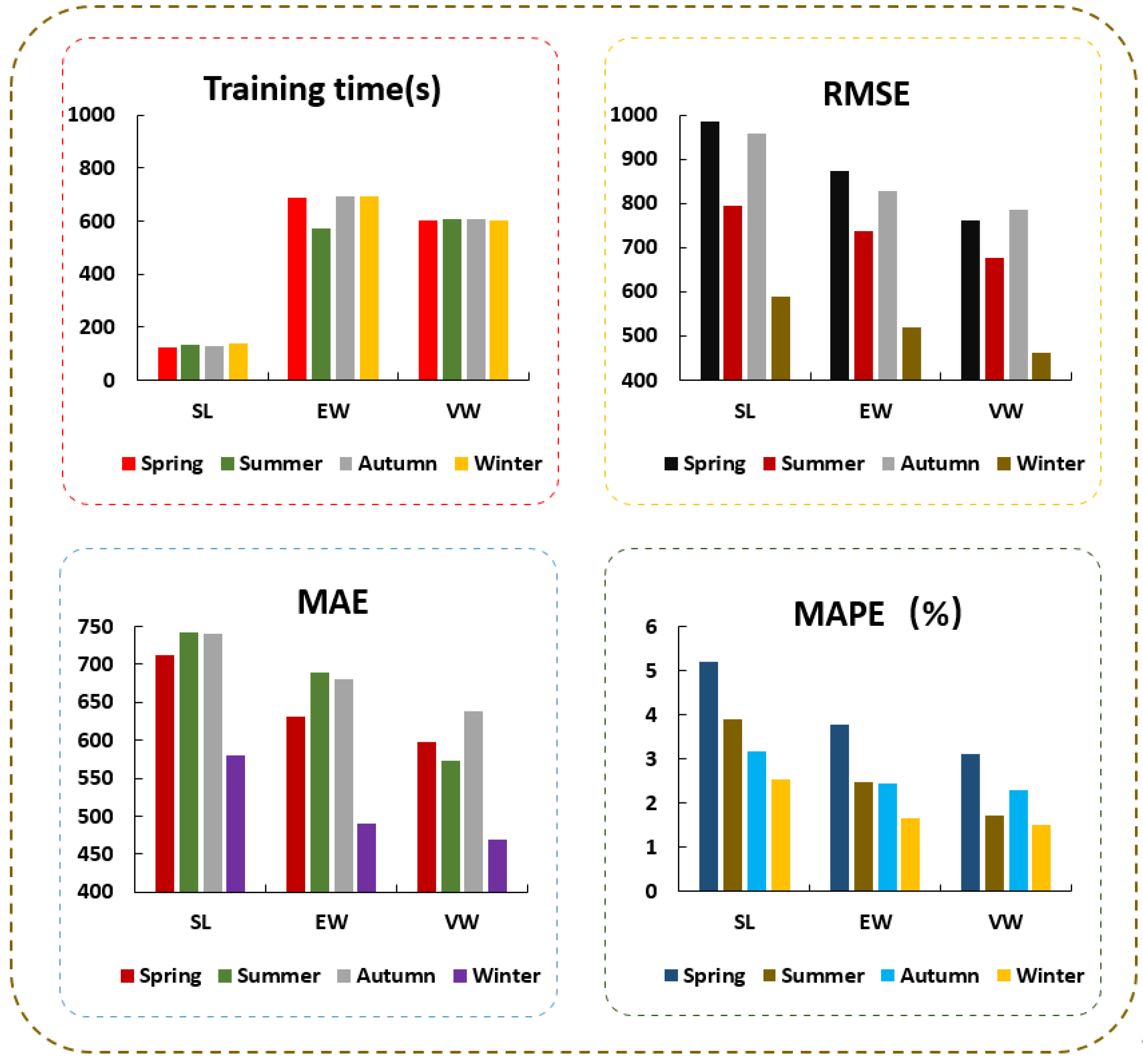
The training speed of the WSLSTM prediction model built by using the weight-sharing mechanism is significantly faster than the traditional LSTM model and GRU model. In addition, the WSLSTM model also has higher prediction accuracy than the traditional LSTM model and GRU model because it can extract common features among the components.

(4)

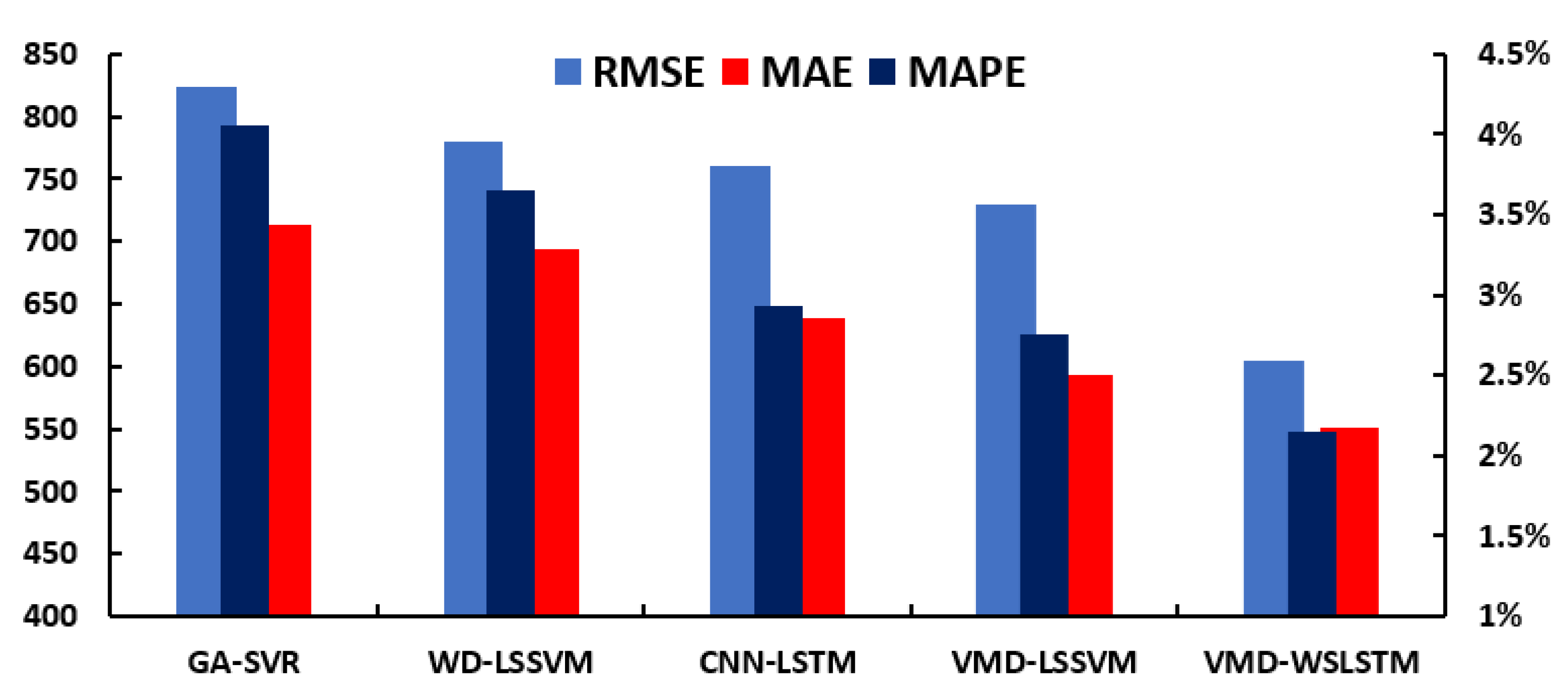
The model in this paper has better prediction accuracy compared with traditional models such as GA-SVR, WD-LSSVM, CNN-LSTM, and VMD-LSSVM.

Therefore, feature selection using Shapley values and the prediction model using the weight-sharing mechanism proposed in this paper can improve the accuracy and speed of the prediction model. However, the model also has some shortcomings. For example, feature selection can take a lot of time when there are more features to be considered. Secondly, the Shapley threshold value when performing feature selection also needs further exploration.

References

1. Jurado, S.; Nebot, A.; Mugica, F.J.; Avellana, N. Hybrid methodologies for electricity load forecasting: Entropy-based feature selection with machine learning and soft computing techniques. Energy 2015, 86, 276–291. [Google Scholar] [CrossRef] [Green Version]
2. Lahouar, A.; Slama, J.B.H. Day-ahead load forecast using random forest and expert input selection. Energy Convers. Manag. 2015, 103, 1040–1051. [Google Scholar] [CrossRef]
3. Chae, Y.T.; Horesh, R.; Hwang, Y.; Lee, Y.M. Artificial neural network model for forecasting sub-hourly electricity usage in commercial buildings. Energy Build. 2016, 111, 184–194. [Google Scholar] [CrossRef]
4. Keles, D.; Scelle, J.; Paraschiv, F.; Fichtner, W. Extended forecast methods for day-ahead electricity spot prices applying artificial neural networks. Appl. Energy 2016, 162, 218–230. [Google Scholar] [CrossRef]
5. Che, J.; Wang, J.; Wang, G. An adaptive fuzzy combination model based on self-organizing map and support vector regression for electric load forecasting. Energy 2012, 37, 657–664. [Google Scholar] [CrossRef]
6. Zhang, Y.; Xiong, R.; He, H.; Pecht, M.G. Long Short-Term Memory Recurrent Neural Network for Remaining Useful Life Prediction of Lithium-Ion Batteries. IEEE Trans. Veh. Technol. 2018, 67, 5695–5705. [Google Scholar] [CrossRef]
7. Kong, W.; Dong, Z.Y.; Jia, Y.; Hill, D.J.; Xu, Y.; Zhang, Y. Short-Term Residential Load Forecasting Based on LSTM Recurrent Neural Network. IEEE Trans. Smart Grid 2017, 10, 841–851. [Google Scholar] [CrossRef]
8. Batchuluun, G.; Nguyen, D.T.; Pham, T.D.; Park, C.; Park, K.R. Action Recognition from Thermal Videos. IEEE Access 2019, 7, 103893–103917. [Google Scholar] [CrossRef]
9. Xie, Y.; Liang, R.; Liang, Z.; Huang, C.; Zou, C.; Schuller, B. Speech Emotion Classification Using Attention-Based LSTM. IEEE/ACM Trans. Audio Speech Lang. Process. 2019, 27, 1675–1685. [Google Scholar] [CrossRef]
10. Nowotarski, J.; Liu, B.; Weron, R.; Hong, T. Improving short term load forecast accuracy via combining sister forecasts. Energy 2016, 98, 40–49. [Google Scholar] [CrossRef]
11. Zhu, G.; Peng, S.; Lao, Y.; Su, Q.; Sun, Q. Short-Term Electricity Consumption Forecasting Based on the EMD-Fbprophet-LSTM Method. Math. Probl. Eng. 2021, 2021, 6613604. [Google Scholar] [CrossRef]
12. Semero, Y.K.; Zhang, J.; Zheng, D. EMD–PSO–ANFIS-based hybrid approach for short-term load forecasting in microgrids. IET Gener. Transm. Distrib. 2020, 14, 470–475. [Google Scholar] [CrossRef]
13. Tang, X.; Dai, Y.; Liu, Q.; Dang, X.; Xu, J. Application of Bidirectional Recurrent Neural Network Combined with Deep Belief Network in Short-Term Load Forecasting. IEEE Access 2019, 7, 160660–160670. [Google Scholar] [CrossRef]
14. Azam, M.F.; Younis, M.S. Multi-Horizon Electricity Load and Price Forecasting Using an Interpretable Multi-Head Self-Attention and EEMD-Based Framework. IEEE Access 2021, 9, 85918–85932. [Google Scholar] [CrossRef]
15. Wang, Y.; Sun, S.; Chen, X.; Zeng, X.; Kong, Y.; Chen, J.; Guo, Y.; Wang, T. Short-term load forecasting of industrial customers based on SVMD and XGBoost. Int. J. Electr. Power Energy Syst. 2021, 129, 106830. [Google Scholar] [CrossRef]
16. Zhou, M.; Hu, T.; Bian, K.; Lai, W.; Hu, F.; Hamrani, O.; Zhu, Z. Short-Term Electric Load Forecasting Based on Variational Mode Decomposition and Grey Wolf Optimization. Energies 2021, 14, 4890. [Google Scholar] [CrossRef]
17. He, F.; Zhou, J.; Feng, Z.-K.; Liu, G.; Yang, Y. A hybrid short-term load forecasting model based on variational mode decomposition and long short-term memory networks considering relevant factors with Bayesian optimization algorithm. Appl. Energy 2019, 237, 103–116. [Google Scholar] [CrossRef]
18. Gendeel, M.; Yuxian, Z.; Aoqi, H. Performance comparison of ANNs model with VMD for short-term wind speed forecasting. IET Renew. Power Gener. 2018, 12, 1424–1430. [Google Scholar] [CrossRef]
19. Qin, G.; Yan, Q.; Zhu, J.; Xu, C.; Kammen, D. Day-Ahead Wind Power Forecasting Based on Wind Load Data Using Hybrid Optimization Algorithm. Sustainability 2021, 13, 1164. [Google Scholar] [CrossRef]
20. Jianwei, E.; Ye, J.; He, L.; Jin, H. Energy price prediction based on independent component analysis and gated recurrent unit neural network. Energy 2019, 189, 116278. [Google Scholar] [CrossRef]
21. Jung, S.-M.; Park, S.; Jung, S.-W.; Hwang, E. Monthly Electric Load Forecasting Using Transfer Learning for Smart Cities. Sustainability 2020, 12, 6364. [Google Scholar] [CrossRef]
22. Ge, L.J.; Xian, Y.M.; Wang, Z.G.; Gao, B.; Chi, F.J.; Sun, K. Short-term Load Forecasting of Regional Distribution Network Based on Generalized Regression Neural Network Optimized by Grey Wolf Optimization Algorithm. CSEE J. Power Energy Syst. 2021, 7, 1093–1101. [Google Scholar] [CrossRef]
23. Liu, D.; Wang, L.; Qin, G.; Liu, M. Power Load Demand Forecasting Model and Method Based on Multi-Energy Coupling. Appl. Sci. 2020, 10, 584. [Google Scholar] [CrossRef] [Green Version]
24. Pei, S.; Qin, H.; Yao, L.; Liu, Y.; Wang, C.; Zhou, J. Multi-Step Ahead Short-Term Load Forecasting Using Hybrid Feature Selection and Improved Long Short-Term Memory Network. Energies 2020, 13, 4121. [Google Scholar] [CrossRef]
25. Tucker, A.W.; Luce, R.D. Contributions to the theory of games. Math. Gaz. 1953, 37, 134. [Google Scholar]
26. Fryer, D.; Strumke, I.; Nguyen, H. Shapley Values for Feature Selection: The Good, the Bad, and the Axioms. IEEE Access 2021, 9, 144352–144360. [Google Scholar] [CrossRef]
27. Dong, H.; Sun, J.; Sun, X. A Multi-Objective Multi-Label Feature Selection Algorithm Based on Shapley Value. Entropy 2021, 23, 1094. [Google Scholar] [CrossRef]
28. Visser, L.; AlSkaif, T.; van Sark, W. The Importance of Predictor Variables and Feature Selection in Day-ahead Electricity Price Forecasting. In Proceedings of the 2020 International Conference on Smart Energy Systems and Technologies (SEST), Istanbul, Turkey, 7–9 September 2020. [Google Scholar] [CrossRef]
29. Lundberg, S.M.; Erion, G.; Chen, H.; DeGrave, A.; Prutkin, J.M.; Nair, B.; Katz, R.; Himmelfarb, J.; Bansal, N.; Lee, S.-I. From local explanations to global understanding with explainable AI for trees. Nat. Mach. Intell. 2020, 2, 56–67. [Google Scholar] [CrossRef]
30. Dragomiretskiy, K.; Zosso, D. Variational Mode Decomposition. IEEE Trans. Signal Process. 2014, 62, 531–544. [Google Scholar] [CrossRef]
31. Hochreiter, S.; Schmidhuber, J. Long short-term memory. Neural Comput. 1997, 9, 1735–1780. [Google Scholar] [CrossRef]
32. Roth, W.; Pernkopf, F. Bayesian Neural Networks with Weight Sharing Using Dirichlet Processes. IEEE Trans. Pattern Anal. Mach. Intell. 2020, 42, 246–252. [Google Scholar] [CrossRef]
33. Aggarwal, H.K.; Mani, M.P.; Jacob, M. MoDL: Model-Based Deep Learning Architecture for Inverse Problems. IEEE Trans. Med. Imaging 2019, 38, 394–405. [Google Scholar] [CrossRef]
Figure 1. Schematic diagram of the structure of the long short-term memory network.
Energies 15 00487 g001
Figure 2. Schematic diagram of WSLSTM prediction model structure.
Energies 15 00487 g002
Figure 3. Structural framework of the proposed model.
Energies 15 00487 g003
Figure 4. Hourly gas load.
Energies 15 00487 g004
Figure 5. Shapley with different seasonal load characteristics.
Energies 15 00487 g005
Figure 6. Experimental prediction results by season.
Energies 15 00487 g006
Figure 7. Prediction results of different feature selection methods.
Energies 15 00487 g007
Figure 8. Prediction results of different decomposition methods.
Energies 15 00487 g008
Figure 9. Forecast results of different forecasting methods.
Energies 15 00487 g009
Figure 10. Prediction results of different models.
Energies 15 00487 g010