Effect of Cell Electrical Mismatch on Output of Crystalline Photovoltaic Modules

Abstract

The importance of energy supply and demand has been emphasized over the past few years. Renewable energy without regional bias continues to attract attention. The improvement of the economic feasibility of renewable energy leads to the expansion of the supply, and the global supply of solar modules is also rapidly increasing. Recently, the price of polysilicon for solar modules is also rising significantly. Interest in recycling waste modules is also increasing. However, the development of cost-effective treatment technology for solar modules that have reached the end of their commercial useful life is still insufficient. We are going to propose the standards necessary to restore and reuse so-called waste solar modules in a more eco-friendly and economical way. A crystalline solar module is an aggregate of individual solar cells. The technology is stable and has good durability. The efficiency of crystalline solar cells has dramatically improved in recent decades. The grade of cell that was mainly used two or three years ago will be discontinued soon. Therefore, electrical mismatch of the cells occurs while repairing an old-manufactured module with recently produced cells. In this paper, we experimentally verify how the increase in cell mismatch affects the module output. We intend to suggest the range of acceptable mismatches by analyzing the tendency. First of all, we repaired and restored the module in which all the existing cells were discontinued after about 10 years of production. The replacement cell had 16.94% higher output than the existing cells. After restoring the module, it was confirmed that the electrical mismatch loss of the cell in this range was very small, about 1.69%. Second, the mismatch loss was confirmed by manufacturing a module by mixing the two cells. The difference in output between the two cells was 5.56%. The mismatch loss compared to the predicted value based on the output of the individual cell and the actual value was very small, less than 0.76%. The long-term reliability results through the DH 1000 hr experiment on the sample that simulated the situation of repair, and the rest of the samples also showed a decrease in output up to 1.13%, which was not a problem. Finally, we hypothesized that a series-connected array should be constructed by reusing modules with different output classes. By cutting into 1/4, 1/3, and 1/2 of cells of the same grade, various unit module samples composed of 0.5 cells to 2.0 cells were manufactured and the output was measured. Electrical mismatch loss was tested by serially combining each unit module at various mismatch ratios. It was confirmed that the output loss in the three or more samples similarly exceeds about 10% with the mismatch ratio of 50% as the starting point. In the previous study, when the mismatch ratio was 70%, the output loss was about 17.98%. The output loss was 18.30% at 86.57%, 17.33% at 77.33%, and 14.37% at 75%. Considering that it is a value measured in a wide range, it is a result that is quite consistent with the results of previous studies. When the cell output difference was less than 50%, the electrical mismatch of the cell had no significant effect on the module output. When it exceeds that, a sudden output loss of 10% or more begins to occur. Consequently, the mismatch range of compatible cells should be less than 50%. If it exceeds that, not only output loss but also safety problems may occur due to heat generation. We can offer a range of interchangeable cell output power when crystalline solar modules are repaired and reused. By recycling modules with different outputs, you can provide a standard for those who want to use it by composing an array. By extending the lifespan of a solar module once used, it is expected that the generation of waste can be reduced from environmental point of view and the resources required to manufacture a new module can be saved from the resource-circulation point of view.

1. Introduction

Recently, the photovoltaic industry has grown into one of the most promising areas of application of renewable energy technologies. The number of solar systems is increasing worldwide [1,2,3,4,5]. The achievement of grid parity is accelerating with the continuous improvement of efficiency and economic feasibility in recent years [6,7,8,9,10,11]. The cumulative installed capacity of solar power worldwide has exceeded 760 GW in 2021. The installed capacity is projected to reach 214 GW in 2022 [12,13]. With the growth of the solar industry, the price of polysilicon is also rising rapidly [14,15]. The recycling market for solar modules is attracting attention due to economic feasibility and environmental reasons [16,17,18]. Expanding the spread of solar power helps to reduce carbon dioxide emissions. The issue of disposal of solar modules has become a new consideration for the environment [19,20,21,22,23]. The focus should be on minimizing the environmental burden due to the disposal of solar systems [24,25].

It is known that solar modules can be used for a long time of 25 years or more [26,27]. The period of subsidy for solar power plants is limited to 15 to 20 years. The commercial shelf life of subsidized utility-scale commercial solar power plants worldwide is gradually expiring. The disposal problem of waste modules arising here can cause serious environmental problems [28,29,30,31]. As announced in the previous study, it is expected that about 80 million tons of waste solar modules will be generated by 2050 [32]. Solar waste modules contain various valuable metals and high-purity glass and silicon wafers. Therefore, the collection and recycling of these waste modules is emerging as an important task for the sustainability of the photovoltaic industry and renewable energy [33]. The technology of crushing solar modules and recycling them as raw materials is not economical. Previous studies have reported that the return on investment (ROI) for this type of recycling technology is less than about −0.25 [34]. A technology that can economically recycle modules is a technology that partially repairs and reuses waste modules. A method of repairing a module by simple replacement of a junction box including diodes, cables, and connectors is commonly used. A technique for repairing the damaged back sheet by coating it with sealant or synthetic rubber was also newly announced [35,36]. A technique for repairing a module by re-soldering the hot-spot of the module’s upper-lower circuit was also introduced [37]. In a previous study, a method of repairing a module by replacing some damaged cells in a waste module with new cells was introduced. Techniques for module reuse have been proposed [38].

In particular, there are things to know when repairing a module by replacing some of the cells of different grades or when composing an array with various types of repaired modules. It is the effect of the electrical mismatch of the cell on the output of the module. Electrical mismatch of cells does not mean within output deviation between cells included in one module. In some cases, it is necessary to design an array by combining several types of repaired modules. Even the results of measuring the output by connecting the module of the 4-inch cell base and the module of the 5-inch cell base in series are well documented in previous studies [39]. In this paper, modules with the same cell series but different wafer sizes are connected in series with different outputs of 85 Wp and 50 Wp. The difference in output is about 70% more for a large module based on a small module. The sum of the individual actual outputs of these modules is 169.42 Wp. The output value connected in series is 138.96 Wp. The difference between the two figures is 30.46 Wp. It has a difference of 17.98% compared to the estimated value. The energy lost here may have been consumed during the transmission of electricity [40]. Most of them are converted into thermal energy in high-output cells, which adversely affects the system [41,42,43]. The range that can be mixed without significantly affecting the theoretical total output was investigated. The experiments were carried out in modules in the earlier investigations. In this study, we describe the cell unit’s mismatch tolerance. This establishes whether cells with some degree of mismatch can be substituted to restore the module’s output. The allowed range of electrical mismatch of cells that can be used in combination was confirmed. This is a very important question for those who want to repair and reuse a module. We may be able to present a mixed range of acceptable cell output for those who wish to restore the module by replacing the cell in our experiments.

2. Experiments

2.1. Methods and Procedures

2.1.1. Theoretical Background to Module Output Analysis

The CTM (cell to module) factor calculation method was applied to the analysis of the output of the cells used at the time of manufacture for the samples to be analyzed. [44,45,46]. Models and formulas for classifying k-factors that affect efficiency or output when manufacturing modules and analyzing loss or gain mechanisms have been presented in previous studies. In the module output calculation model, the module output is calculated from the sum of the CTM coefficient k and the individual cell output when manufacturing the module. The basic formula for the module output is shown as Equations (1) and (2) below. The module margin is the distance between the cell matrix and the outside of the module frame. Cell spacing refers to the distance between cells within a string.

Table 1. Explanation of symbols and abbreviations used in the CTM method.

Symbols	Explanation	Symbols	Explanation
l, m	π function variable	k1	Module margin
k2	cell spacing	k3	cover reflection
k4	cover absorption	k5	cover/encapsulant reflection
k6	encapsulant absorption	k7	interconnection shading
k8	cell/encapsulant coupling	k9	finger coupling
k10	interconnector coupling	k11	cover coupling
k12	cell interconnection	k13	string interconnection
k14	electrical mismatch	k15	junction box and cabling

shows the description of symbols and abbreviations used in the formulas below.

$${\eta }_{module}=\frac{P_{module}}{E_{STC}·\left(A_{margin}+A_{cell spcing}+A_{cells}\right)}$$

(1)

$${\eta }_{module}={\overline{\eta }}_{cell}·\left(k_1+k_2-1\right)·{\displaystyle \prod }_{i=3}^m{k}_i$$

(2)

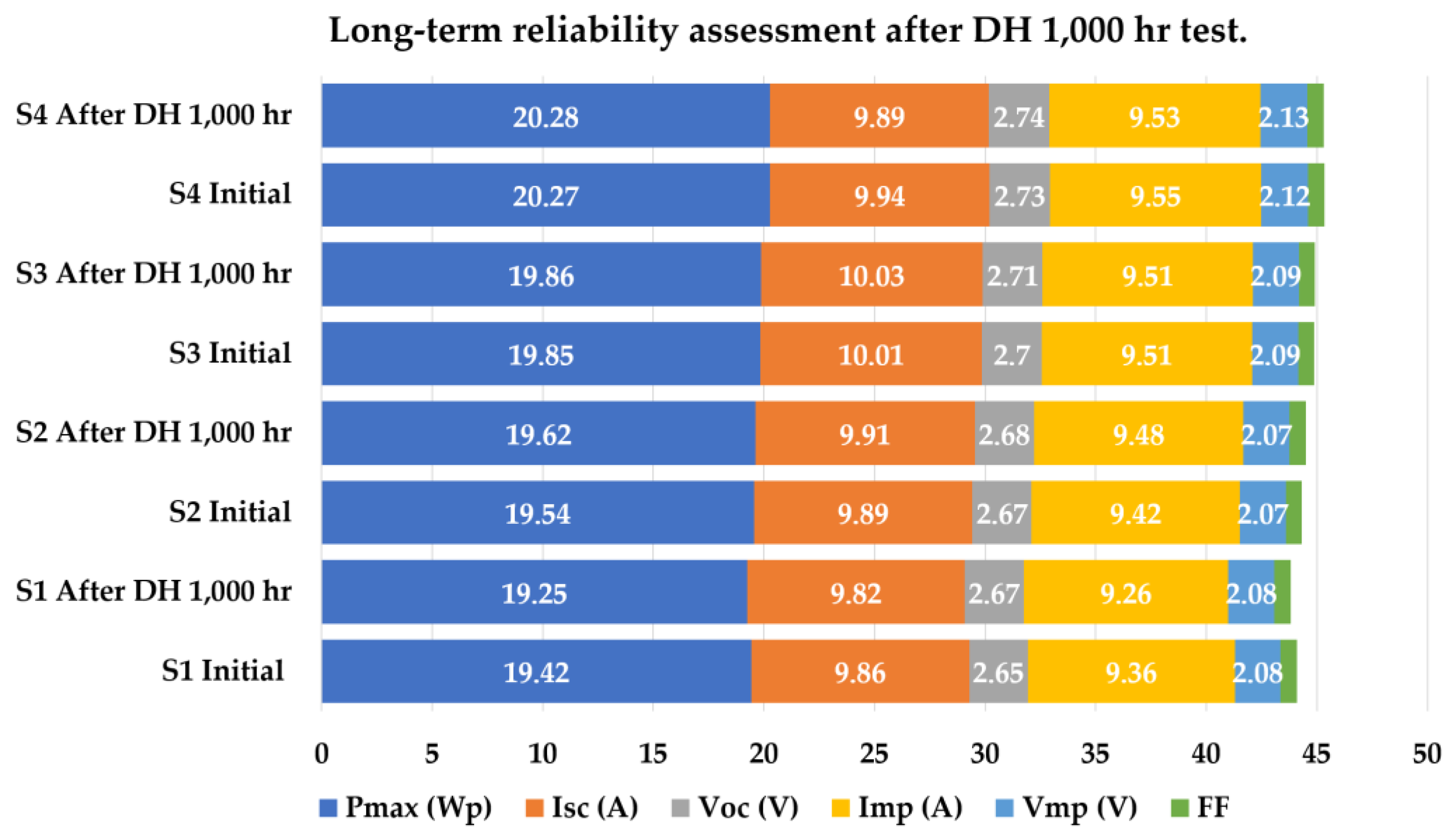
Equation (2) states that the efficiency of the module is proportional to the average value of the efficiency of individual cells. This means that the efficiency of the modules connected in series is proportional to the average efficiency of the entire cell, rather than being downwardly leveled by the dominant influence of the least efficient cell due to a ‘bottleneck’. The output of the module to be restored can be predicted by calculating the average efficiency of the cell in consideration of k14 (cell electrical mismatch loss). It can be concluded that the difference between this predicted value and the actual experimental value is the sum of the long-term degradation of the cell and the loss of electrical mismatch, which can only be calculated as a final value [47]. These two values can be separated from long-term degradation by additional experiments using mismatch of new cells.

The loss due to the electrical mismatch of the cell has been published as a concept called RPL (relative power loss), which is not precisely defined and classified before the CTM factor [48]. RPL is expressed as the difference between the maximum power (Pmpc) of n individual cells connected in series to form a cell string or module and the output power of the cell string. Relative power loss can be expressed as Equation (3) below from the difference between the sum of the maximum power of n cells and the maximum power of the module.

$$RPL=\frac{{{\displaystyle \sum }}_{i=1}^n·P_{mpci}-P_{module}}{{{\displaystyle \sum }}_{i=1}^n·P_{mpci}}$$

(3)

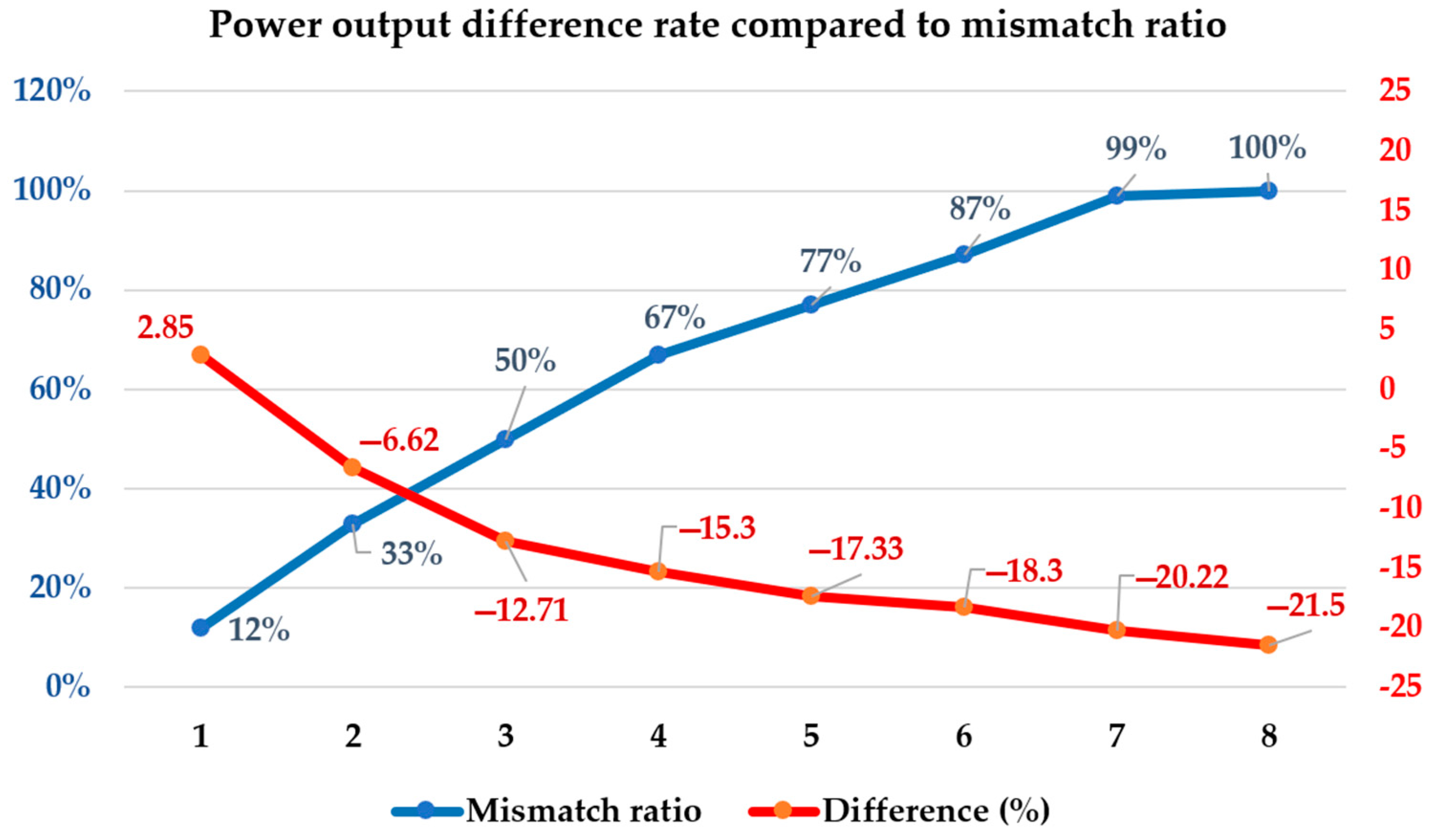
In a situation where the electrical output deviation of the cell is not large, RPL including electrical mismatch is insignificant. In the mismatch range that does not exceed a certain level, it is more dominantly influenced by the arithmetic mean value of the cell rather than the bottleneck or down-leveling. This will be covered in more detail in the Results and Discussion section.

In general, the above formula is used to calculate the efficiency of a module. Among the 15 CTM factors in the output of the module, the overall dimension of the module or the gap between cells does not increase the output of the module, nor does it affect the output by absorbing or reflecting the output [49]. The two factors only affect the areal efficiency of the module. Subtracting is correct when calculating the module output. This is because the design margin (k1) of the module for securing the insulation distance and the loss factor (k2) due to the cell spacing do not affect the output. Equations (3) and (4) below are formulas for calculating the output from the module.

$$P_{module}={\displaystyle \prod }_{i=3}^m{k}_i·{\displaystyle \sum }_{j=1}^n·P_{cell·j}$$

(4)

$$CT{M}_{power}={\displaystyle \prod }_{i=3}^m{k}_i$$

(5)

The expression for CTM power is the output of a pure module and can be expressed as Equations (3) and (4). This is a method of calculating the output of the cell applied in the manufacturing stage of each module using Equations (3) and (4). The procedure for calculating long-term degradation after applying a replacement cell during module repair will be described later in the Results and Discussion section.

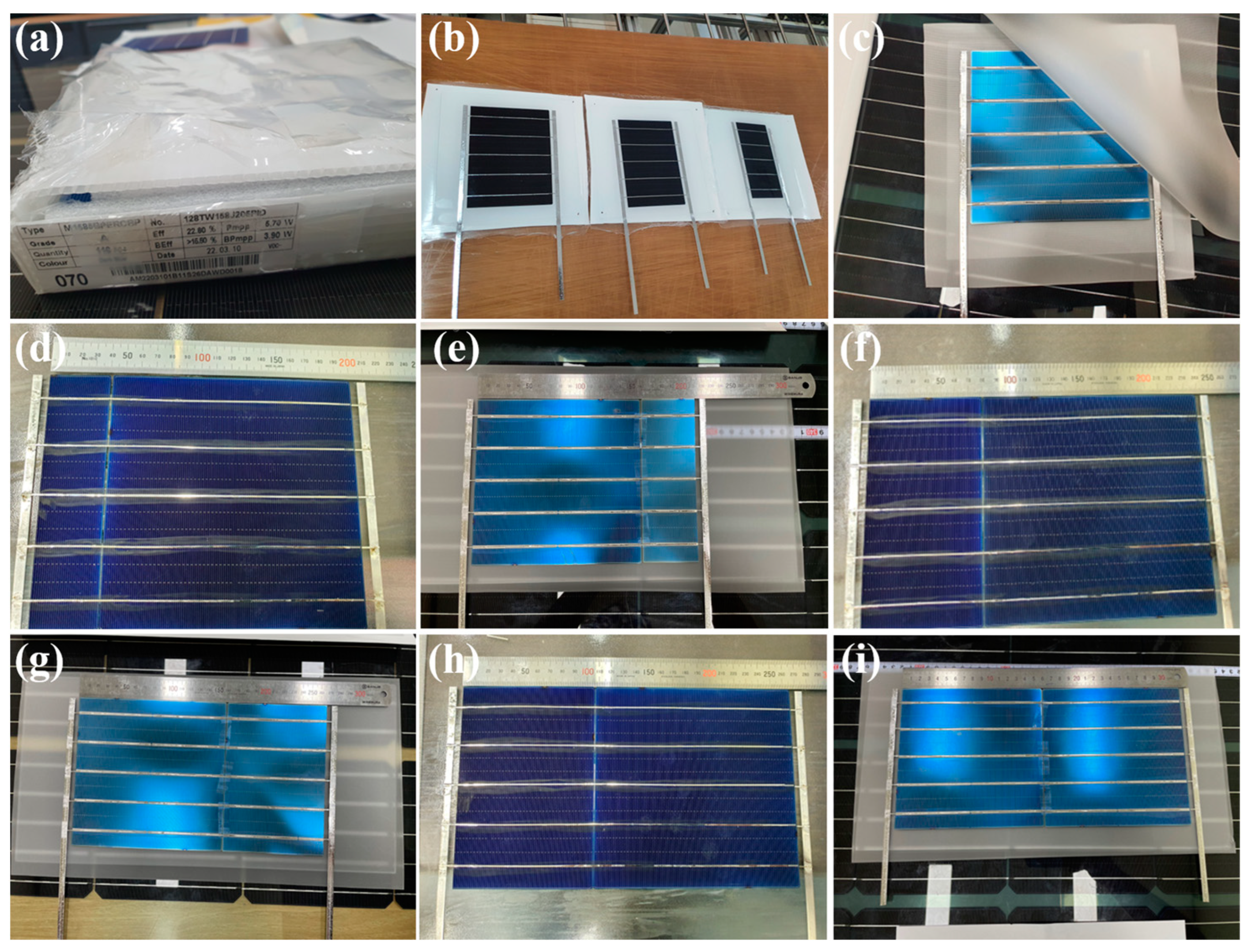
2.1.2. Basic Experiment According to Previous Research Procedure

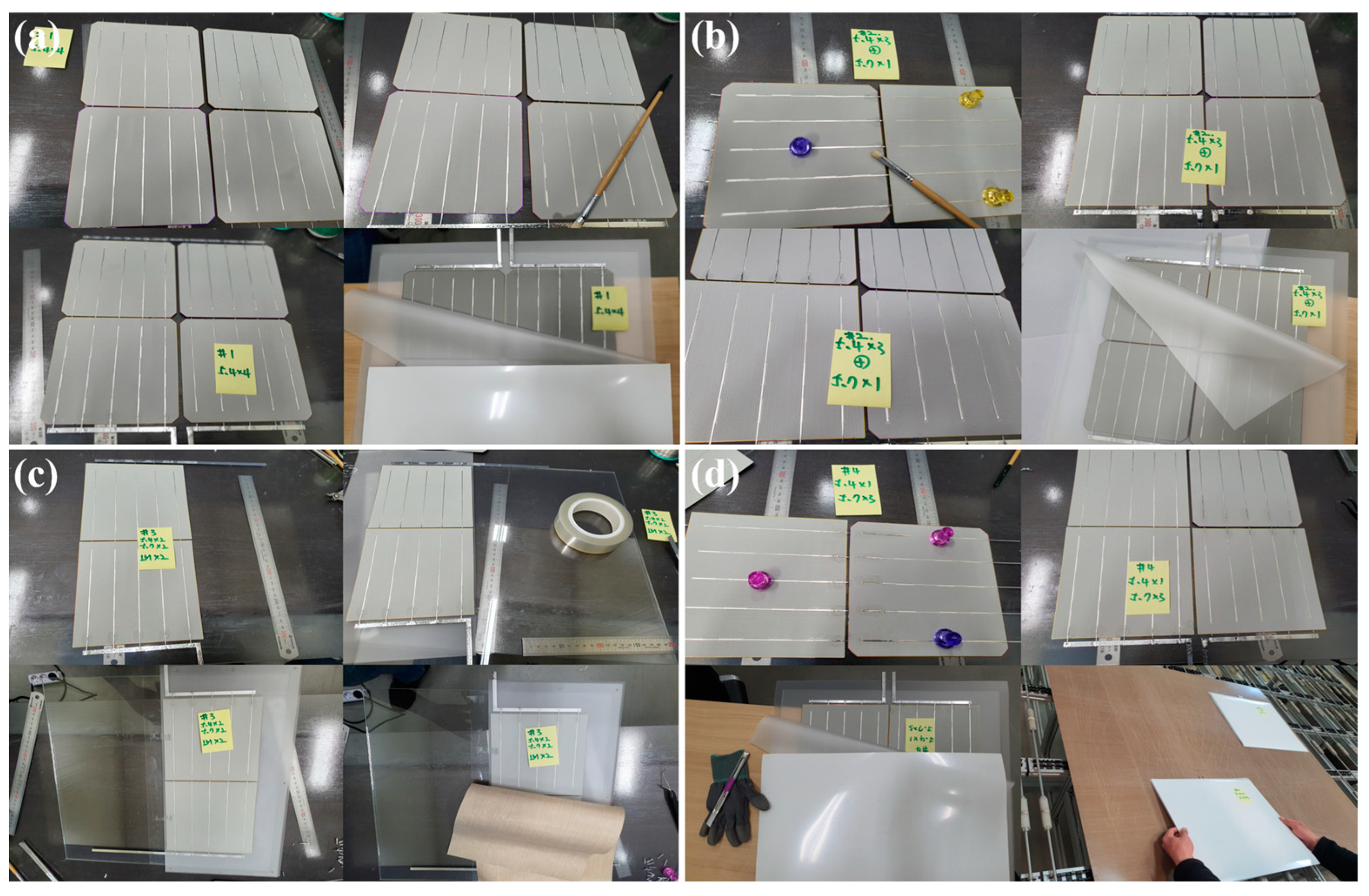
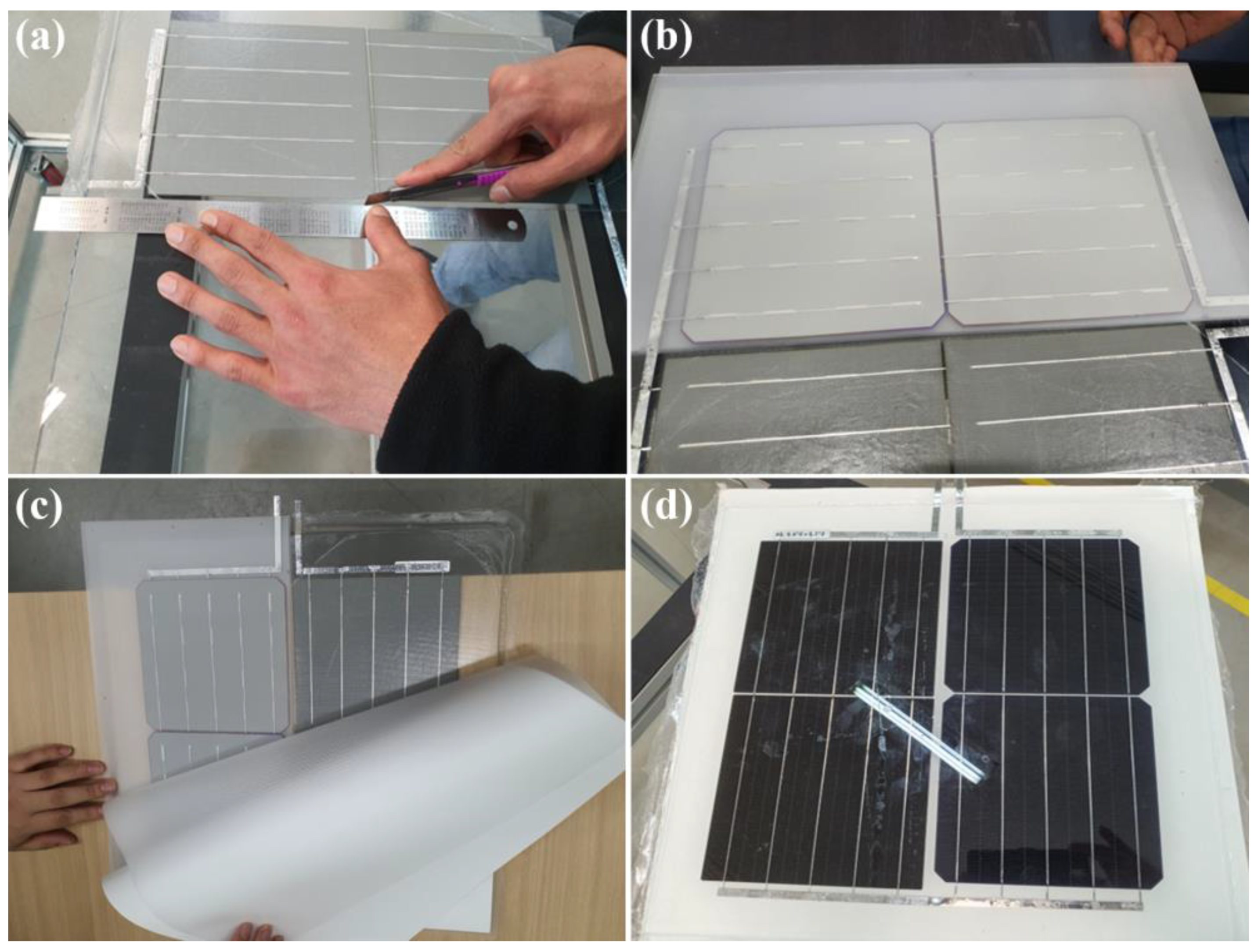
In a previous study [48] that reported repairs of a waste module containing some damaged cells by replacing it with a new cell, it which was checked whether the same results were obtained even when the module type was different as a single crystal. The cell replacement experiment followed the sequence from previous studies. An EL measurement was carried out, and the frame and junction box were removed. The back sheet was also removed by heating on a hot plate. Then, the cells were replaced by using a scraper. Repairment was carried out as shown in Figure 1 through lamination. 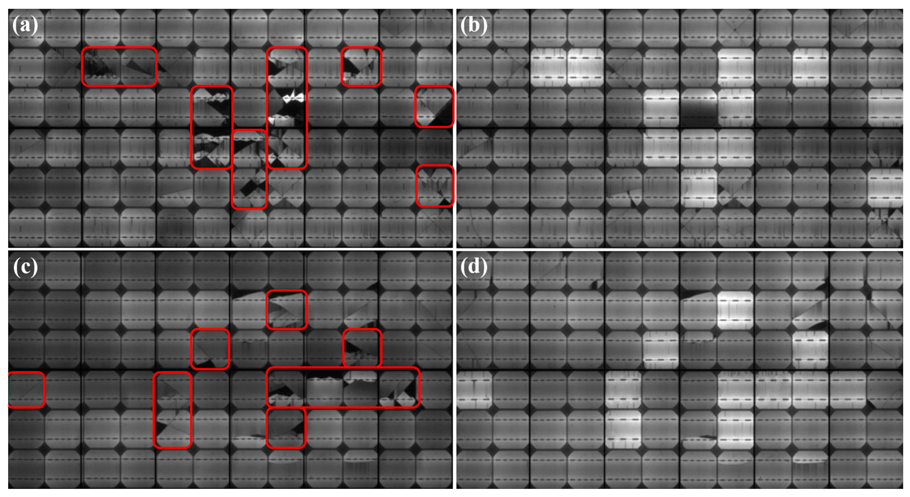Figure 1 is an EL image before and after repair of a 175 WP class single-crystal solar module.

Figure 1a is an EL image before repair of a 175 Wp-class single-crystal solar waste module whose output has significantly dropped due to cell-in-hotspot. For convenience, this sample will be referred to as 175A. The black inactive area of the cells in the red mark is electrically isolated and thus the amount of power is lost. Most of the cells in the middle are dead areas, the reverse current is generated, and the output is severely degraded. Figure 1b shows EL image after repair by replacing the damaged cell of the 175A module next to it. Overall, the hotspot has been greatly alleviated. A hotspot that occurred during the repair process was seen in the bus bar of one cell that was not replaced. The slight decrease in output due to this will be compared again by looking at the current-voltage (I-V) characteristic curve later. Figure 1c also shows an EL image before repair of a 175 Wp class waste module of which the output was lowered due to damaged cells. This module is called 175B. This module also partially contains the dead area of the cell. Repair the module by replacing the cell in this part with a new cell. Figure 1d is an EL image after repair of the 175B module. This module has been fully restored without any defects that occurred during the repair process. The samples above are from commercial power plants. Since there is no I-V data for individual modules at the time of manufacture, the electrical characteristics of the models published on-line by the manufacturer were assumed as initial characteristics.

Table 2. Electrical characteristics of 175A and 175B samples at each stage.

			Pmax (Wp)	Isc (A)	Voc (V)	Imp (A)	Vmp (V)	FF	Tolerance
175A	72 cells	initial	175.00	5.23	44.70	4.90	35.80	0.75	±3%
		failed	149.30	5.22	44.15	4.21	35.45	0.65
			−16%	−0.19%	−1.34%	−14.08%	−99.02%	−13.33%	difference
		repaired	178.57	5.34	44.64	4.98	35.87	0.75
			+16.33%	+21.03%	−0.13%	+3.75%	+0.20%	-	difference
175B	72 cells	initial	175.00	5.23	44.70	4.90	35.80	0.75	±3%
		failed	146.18	5.11	44.18	3.95	37.03	0.65
			−16.47%	−2.29%	−1.19%	−19.18%	+3.43%	−13.33%	difference
		repaired	176.02	5.26	44.65	4.78	36.81	0.75
			+0.58%	+0.57%	−0.01%	−2.45%	+2.82%	-	difference

shows the initial electrical characteristics of the 175A and 175B samples, the characteristics when the output is dropped due to cell damage, and the changes in the electrical characteristics after repair.

The electrical specifications when the sample was first commercially produced were defined as the initial state. In a commercial power plant, the state in which the output is lowered after operating for a certain period of time is set as failed. A sample restored by replacing some damaged cells with new cells was defined as a repaired module stage. In both samples, the output was decreased by about 16% overall. This is similar to about 16.67%, which is the ratio of one string consisting of 12 cells to a module consisting of 72 cells. In other words, it proves that the bypass diode is still sound. If the bypass diode is short-circuited, both strings connected together should come out in black shade. As a result, the output of the module had to drop to about 32%. As confirmed in the EL image, the output degradation is severely observed by damaged cells in the middle of the string.

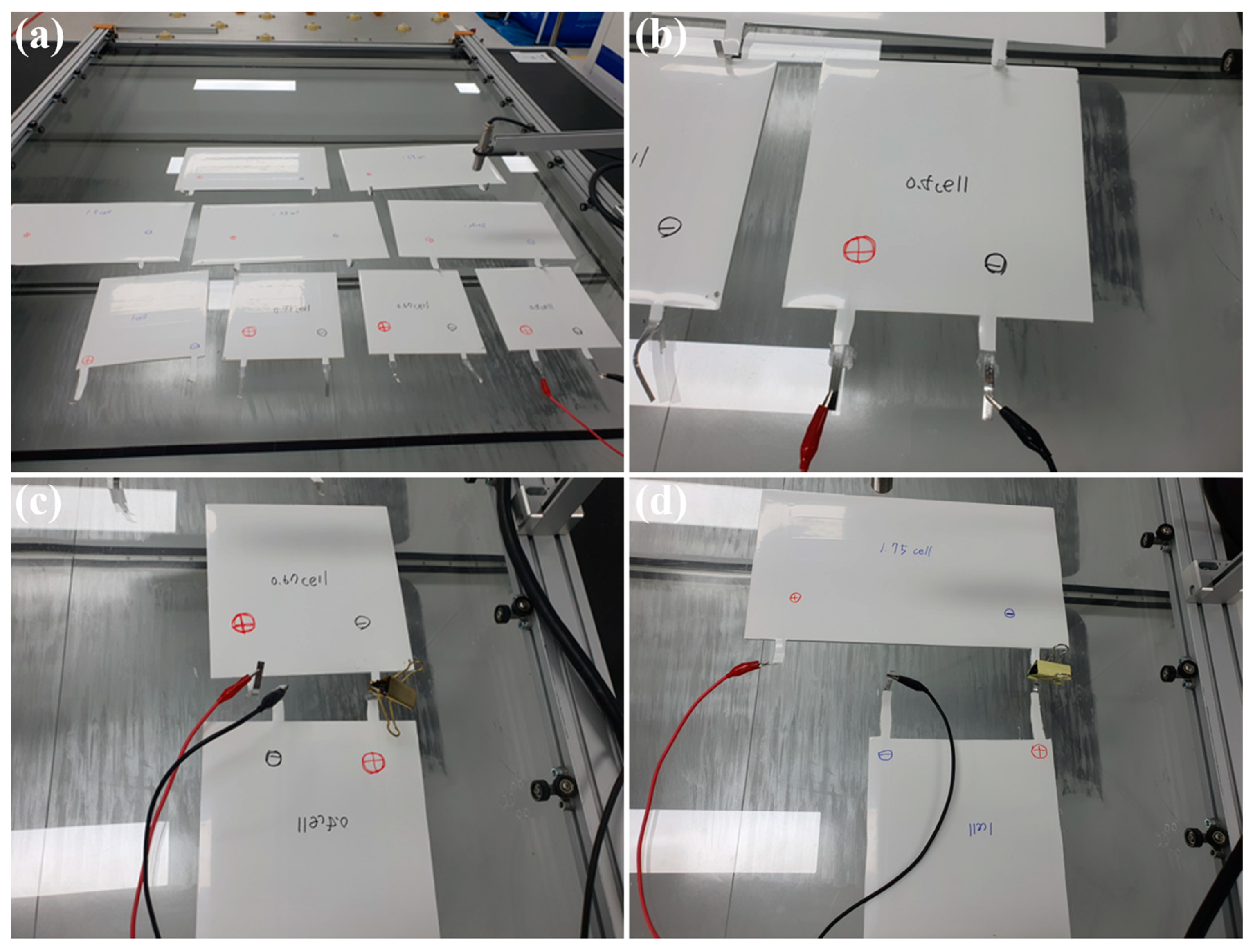
Three factors must be inferred from the above results. First, it is necessary to find out the output of cells by using which the module was manufactured when 175A and 175B samples were commercially produced. Even for the initial model, there is a tolerance of ±3%. In fact, it is most accurate if there is data for each individual module. However, it is a model that has already been produced for more than 10 years, and there is no output data left at the time of production. It is assumed that the electrical characteristics of the module disclosed on-line by the manufacturer are the initial characteristics of the module. Figure 2 shows the I-V and V-P curves before and after repair of the 175A module. The IV curve of the cell-in-hotspot module falls in a stepped shape. The slope of the step is proportional to the degraded output. The V-P curve also shows two or more typical multi-peaks. This is caused by a cell-in-hotspot in the cell string that lowers the short circuit current (I_sc) of the cell and increases the resistance.

The CTM factor analysis method is a method of calculating whether output loss and gain are made at each stage of the module manufacturing process while manufacturing a module with individual cells. Results vary depending on the type of cell. We use this method to inversely compute the output of the initial cell from the module output. This procedure is also important information in order to calculate the annual cell output decline through the resultant value. The grade of the replacement cell applied at the time of repair is already known.

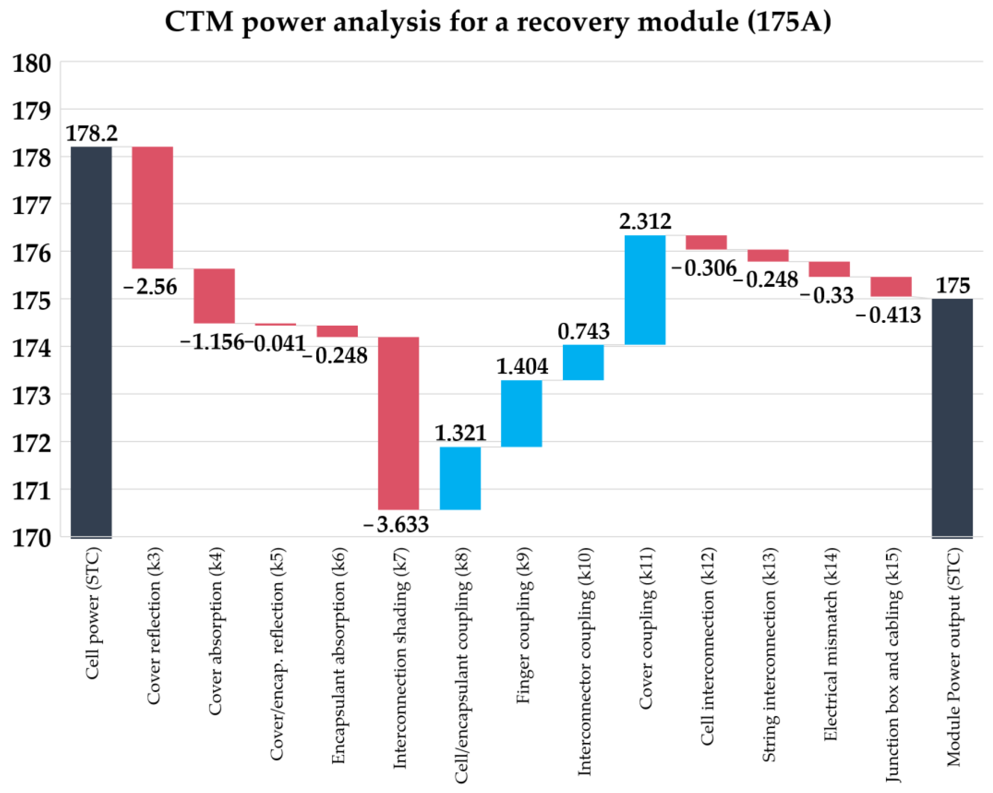
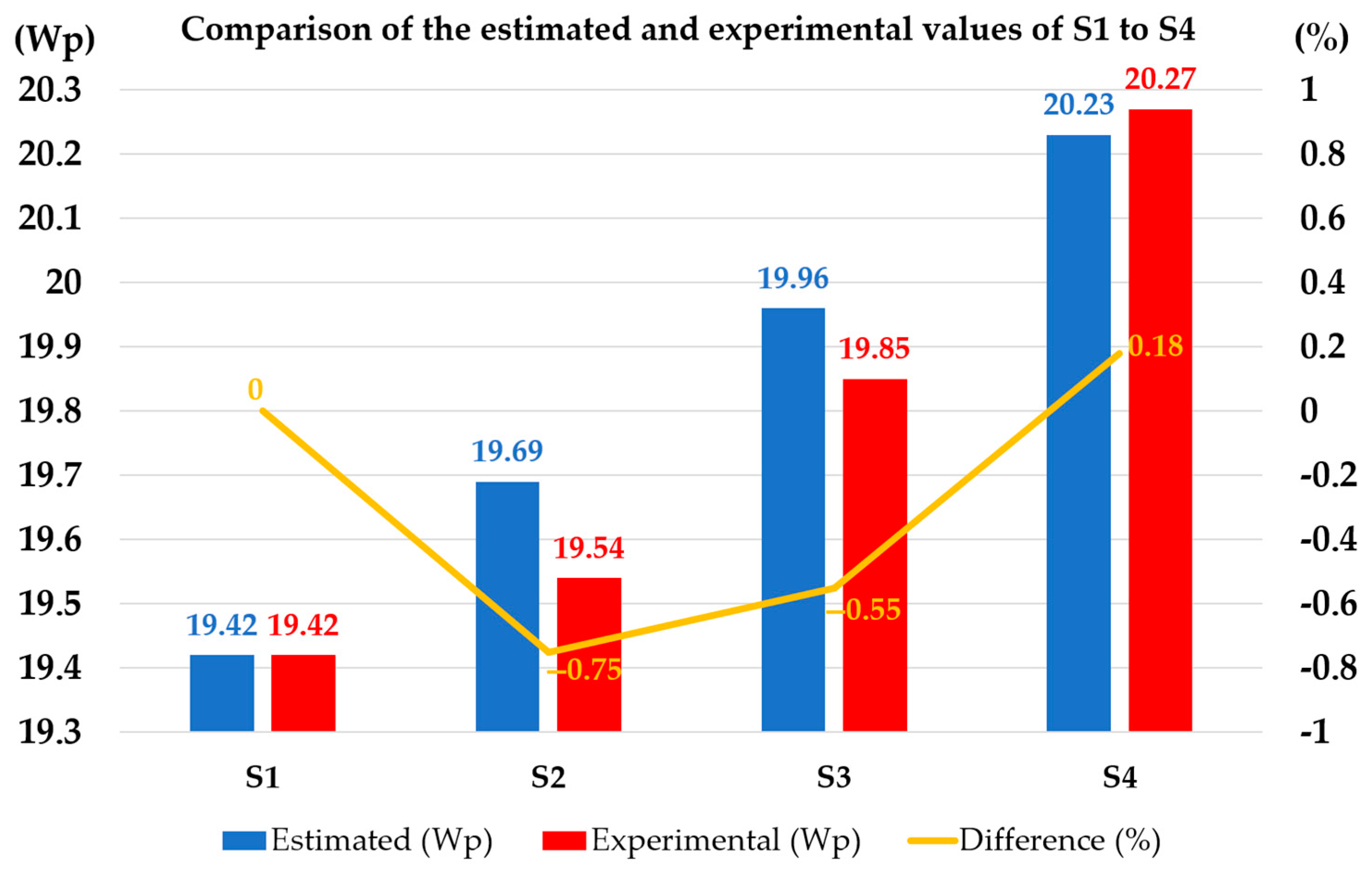
After adding the remaining CTM factors to the value to which the annual degradation is applied to the cells that have not been replaced, the total value of the predicted output of the actually repaired module is calculated if the CTM factor is applied in common. In this case, a loss that is lower than the predicted output value can be classified as a loss due to electrical mismatch of the cell. Figure 3 is the sum of the initial output values of the cells calculated from the module. It is assumed that there is no initial tolerance value at the time of manufacturing the module. Since it is a module at the time of production, if the annual output decrease is calculated as ‘0’, the sum of the output of 72 cells is calculated as 178.2 Wp. Therefore, the output of each cell is 178.2÷72 = 2.48 Wp.

The replacement cell used for repair has a higher output due to technological advances in the past. The power of the cell used for repair is 2.90 Wp. The output is about 17% higher than the 2.48 Wp output of the initial cell. The electrical characteristics of the initial cell and replacement cell are shown in

Table 3. Electrical characteristic deviation of the initial and replacement cells.

Item	Eff. Cell	Pmax (Wp)	Isc (A)	Voc (V)	Imp (A)	Vmp (V)	FF	Tolerance
Initial cell	16.30	2.48	4.94	0.63	4.53	0.55	0.80	±3%
Replacement cell	18.70	2.90	5.66	0.64	5.21	0.56	0.80	±3%

. The tolerance of the initial cell also followed the value of the module’s specification-sheet. The values in the table below are rounded to the third decimal place.

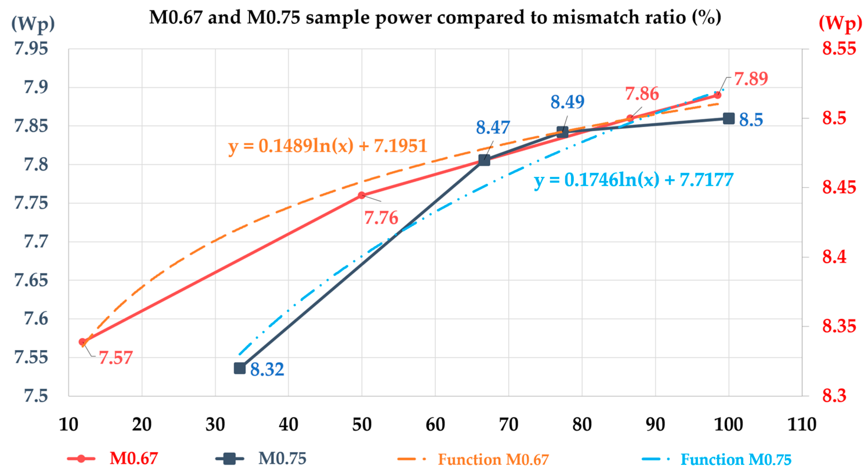
The electrical output of the two cells differs by about 17% in Table 3. If the output of the cells is down-leveled due to the so-called “bottleneck” when manufacturing a module by mixing two cells, the output of the module should not exceed 175 Wp no matter how high the cells are mixed. However, the experimental result was 178.57 Wp for the 175A sample and 176.02 Wp for the 175B sample. Annual output decline rate was considered. In the output of the module, the decrease in output due to the electrical mismatch of the cell is proof that it works limitedly. In addition, the output of the module is proportional to the average value of the individual cell outputs. This is consistent with the result of Equation (2) above. We paid attention to this result and tested how the electrical mismatch of the cell affects the module output to what extent and in what pattern.

2.2. Experimental Details

2.2.1. Effect of Electrical Mismatch on the Output of the Module in a Relatively Small Range (within 10%)

In the experiment, a sample was prepared by applying the initial cell at 5.4 Wp and the replacement cell at 5.7 Wp. Only 5.4 Wp cells without mismatch were used to construct 4 cells-module and used as a control. Figure 4 below shows the production process of the sample produced for the experiment.

Figure 4a was prepared with 4 cells of 5.4 Wp for the control group. This sample was named S1. Figure 4b shows that 3 sheets of 5.4 Wp and 1 sheet of 5.7 Wp cell were mixed. This sample was named S2. Figure 4c was designed to produce 2 sheets of 5.4 Wp by mixing with 2 sheets of 5.7 Wp. The sample was referred to as S3. The sample S3 was produced by a slightly different process. The description of the subsequent manufacturing process of the sample S3 will be described as shown in the following Figure 4c. Figure 4d is produced by mixing 1 sheet of 5.4 Wp with 3 sheets of 5.7 Wp and it is called sample S4. Cell mismatch was tested by fabricating modules with cells that had different outputs. All samples from S1 to S4 used the same 4.0 mm low iron tempered glass. There is no deviation due to use of the same Ribbon, EVA, and back sheet. The only factors affecting the output of the module are the sum of output of each cell and the loss due to mismatch. The difference between the sum of the calculated outputs and the experimental results will be dealt with in the following Results and Discussion section. Figure 5 shows the subsequent manufacturing process of the sample S3.

Figure 5 shows the process of repairing by replacing some cells of the module. Figure 5a depicts the removal of some cells from the existing module. Only half of the module was manufactured, and the lamination was performed. EVA interface of the module and windshield were cleaned with alcohol. Flux was applied to the remaining rear bus bar. The cells to be replaced were connected as shown in Figure 5b. The first EVA sheet was inserted into the front of the replacement cell. The second EVA sheet was placed on the back and fixed so that it did not move. Figure 5c shows that the entire back of the repaired module was covered with EVA and back sheet to finish. Figure 5d shows the module in which the process shown in Figure 5c was finished and the sample was laminated once again. It showed a well-restored result in appearance without bubbles or discoloration at the interface. This method follows the method of restoring the module after replacing the cell in the previous study. Half of the repaired and restored module went through the lamination process only once. The existing area went through two high-temperature lamination processes. To test the long-term reliability of this part, a damp heat 1000 h test was performed [50,51,52,53]. Other samples and controls were also tested for long-term reliability due to output deviation. The initial output and the output decrease after the test were compared. Differences from losses due to electrical mismatch and long-term reliability test results are discussed in the Results and Discussion section.

2.2.2. Effect of Electrical Mismatch on the Output of the Module over a Relatively Large Range (~100%)

When the deviation of the cell output was 17%, the decrease in the output of the module was not large. A wider range of experiments was needed. It is impossible to simultaneously obtain cells where the output deviation of individual cells is 25% to 100%. Cells of the same grade were cut and connected in parallel to fabricate unit cells showing various outputs. Figure 6 shows the manufacturing process of unit modules with various output deviations used in the experiment.

Figure 6a shows the electrical specifications of the cell manufactured in the unit module. The cell type is PERC M3 bifacial. Sunny side (front) output is 5.7 Wp, and cell efficiency is 22.60%. The cell was cut into 1/4 cut, 1/3 cut and 1/2 cut to make a piece cell of 0.25 cell + 0.75 cell, 0.33 cell + 0.67 cell, and 0.5 cell + 0.5 cell. A unit module with various output deviations were manufactured by combining a fragment cell and a single cell. Figure 6b shows a unit module made using 1/2 (0.5) cells, 2/3 (0.67) cells, and 3/4 (0.75) cells. These samples were named M0.5, M0.67, and M0.75 samples. Figure 6c shows the back side of the cell before the lamination of a 1-cell module made using a single cell. A bifacial cell had different color on the front and back of the cell. The front side of the cell was dark blue, and the back side was relatively light blue. This module was called M1.0 sample. Figure 6d is a 1.25 cell module made by connecting 0.25 cell and 1 cell in parallel, and it is the front side of the cell before lamination process. In general, crystalline silicon solar cells are based on the fact that Isc and Imp increase as the efficiency increases. In this case, the area of the module is precisely proportional to the output of the module. This module is named M1.25 sample. Figure 6e is a back view of the M1.33 sample before lamination. This module was manufactured by connecting 0.33 cell and 1 cell in parallel. Figure 6f is a front view of the M1.5 sample made with 1.5 cells before lamination. Figure 6g shows the back view of the M1.67 sample before lamination process. Figure 6h,i are front and back views of the M1.75 and M2.0 samples before lamination process. Figure 7 shows the output measurement by the individual output of the manufactured unit module and the series configuration of various combinations.

Figure 7a shows the output of the manufactured unit module samples arranged to measure the output by the simulator. On the reverse side of the sample, the cells used and their respective polarities are indicated. These marks provide the convenience of not having to check the front side when connecting in series in various combinations. The samples were measured in a simulator under standard test conditions (STC) at 25 °C, 1 Sun (1000 W/m²), and air mass 1.5. The equipment used was a G-Sola sun simulator and was calibrated under AAA conditions in three evaluation items of uniformity, stability, and spectrum. Figure 7b shows the individual output measurement of the M0.5 sample module made of 0.5 cells. Figure 7c shows the electrical mismatch measurement for the series combination of M0.5 and M0.67 samples. The electrical mismatch of a cell is expressed as a percentage by dividing the difference between a cell with a high output and a cell with a lower output based on the cell with a low output. In this figure, the deviation of the output is 0.67 − 0.5 = 0.15, and the mismatch ratio is 0.15 ÷ 0.5 = 0.3, so it is expressed as 30%. Figure 7d is a series-connected mismatch output measurement of the samples M1.0 and M1.75. In the same way, the mismatch rate is expressed as 75%.

3. Result and Discussion

3.1. Basic Experimental Results

Cell replacement was performed in the module consisting of 72 initial cells each of 2.48 Wp. The 12 cells of 175A sample and 11 cells of 175B were replaced with 2.90 Wp grade.

Table 4. Calculation of theoretical output values for each step of 175A/175B sample.

CTM Factor (k)	Initial CTM	175A (Estimated)	175B (Estimated)
Module Power (STC)	175.00	179.95	179.53
k15 (junction box and cabling)	−0.41	−0.42	−0.42
k14 (electrical mismatch)	−0.33	−0.34	−0.34
k13 (string interconnection)	−0.25	−0.25	−0.25
k12 (cell interconnection)	−0.31	−0.31	−0.31
k11 (cover coupling)	2.31	2.38	2.37
k10 (interconnector coupling)	0.74	0.76	0.76
k9 (finger coupling)	1.40	1.44	1.44
k8 (cell/encapsulant coupling)	1.32	1.36	1.36
k7 (interconnection shading)	−3.63	−3.74	−3.73
k6 (encapsulant absorption)	−0.25	−0.25	−0.25
k5 (cover/encapsulant reflection)	−0.04	−0.04	−0.04
k4 (cover absorption)	−1.16	−1.19	−1.19
k3 (cover reflection)	−2.56	−2.63	−2.63
Cell Power (STC)	178.15	183.19	182.77

shows the predicted values for the experimental results after applying the replacement cell to each sample.

The loss value due to electrical mismatch of the cell was obtained by excluding the annual output decrease rate and initial tolerance from the theoretical value was analyzed [54,55,56]. In order to obtain the initial tolerance of the cell, the next additional experiment was performed. The electrical mismatch index of k14 cell is applied to the mismatch of cells already sorted within ±3% when the module was initially manufactured. It should be noted that this is different from mismatch in the range of 3% or more. In general, the annual output degradation rate guaranteed by the module manufacturer is 0.7%/year. This figure is the guaranteed limit for power generation loss due to the failure of some modules in the power plant. In fact, the figures published in the previous study [49] show that 80% or more of crystalline solar modules that have been in operation for more than 10 years only deteriorate by an average of 0.27%/year. However, the actual output degradation is much less. The total decline rate was calculated elsewhere and applied instead of the annual rate. The long-term output degradation rate may vary depending on the type and efficiency of the cell. In this paper, this value was applied and calculated. The output deviation between the replacement cell and the initial cell is 2.9 Wp − 2.48 Wp = 0.42 Wp. This figure represents a mismatch of about 16.94% compared to the output of the existing cell. The sum of the initial total output of the 175A sample in which 12 cells were replaced is 178.15 + (0.42 × 12) = 183.19 Wp. The sum of the initial cell output of the 175B sample is 182.77 Wp. The expected output of the module considering the CTM factors is 179.95 Wp for 175A sample and 179.53 Wp for 175B sample as shown in Table 4. The long-term degradation of 60 cells without replacement in the 175A sample was 2.48 Wp × 60 × 0.27% = 0.4 Wp. The expected output considering the long-term output degradation of the 175A sample is 179.55 Wp. The long-term output decline of the initial 61 cells of 175B is 0.41 Wp, and the expected output is 179.12 Wp.

$$P_{reuse module}={\displaystyle \prod }_{i=3}^m{k}_i·\left(\alpha ·{\displaystyle \sum }_{e=1}^n{P}_{cell,e}+{\displaystyle \sum }_{\gamma =1}^l{P}_{cell,\gamma }\right)$$

(6)

Multiply the initial output of the existing cell by the long-term degradation rate to obtain the total output of the existing cell (n sheets) and add it to the total output of the replaced cell (l sheets). The expected output for the repaired module can be calculated by multiplying the total output of the old and replaced cells by the CTM factor. The output of the 175A sample is 178.57 Wp after the actual power measurement and repair. The output of the 175B sample is 176.02 Wp.

Table 5. The difference between the estimated and the experimental value of 175A/175B.

Sample	Failed (Wp)	Estimated (Wp)	Experimental (Wp)	Difference
175A	149.30	179.55	178.57	−0.98 Wp (−0.55%)
175B	146.18	179.12	176.02	−3.1 Wp (−1.76%)

compares the output of each sample before the repair and the measured value after the actual experimental repair with the theoretically calculated estimate.

Table 5 shows that the difference from the actual value based on the calculated value is very small. This result means that the electrical mismatch between the cell used for repair of the 175A sample and the 175B sample and the cell in the existing module had little effect on the output of the module. However, there is also an error range of ±3%, which is the initial tolerance value that could not be confirmed. Therefore, we verified this part by intentionally manufacturing electrical mismatched samples in the range that exceeds the initial tolerance value of 3% and does not exceed 10%.

3.2. Output and Long-Term Reliability Test Results in a Low Range (5.56%) of Electrical Mismatch

The second experiment is to analyze the experimental results of electrical mismatch of the cell on the output of the module in a relatively smaller range. The important point here is that the mini module of four cells had a low V_oc and a small area. Therefore, CTM analysis as shown in Table 4 cannot be applied. Therefore, the output was measured by making a standard module. Calibration was performed while measuring the output of the same series module based on it. It was decided to measure and calibrate the CTM by using the S1 sample without electrical mismatch as a reference module by making cells of the same grade. The resulting outputs of the experiment are shown in

Table 6. The difference between the estimated and the experimental values of the samples S1–S4.

Sample	Module Configuration	Estimated (Wp)	Experimental (Wp)	Difference
S1	5.4 Wp × 4	19.42	19.42	Standard
S2	(5.4 Wp × 3) + (5.7 Wp × 1)	19.69	19.54	−0.15 Wp (−0.76%)
S3	(5.4 Wp × 2) + (5.7 Wp × 2)	19.96	19.85	−0.11 Wp (−0.55%)
S4	(5.4 Wp × 1) + (5.7 Wp × 1)	20.23	20.27	0.04 Wp (0.18%)

.

Figure 8 shows the comparative analysis of the results in Table 6. The sample S1 consists of 4 5.4 Wp sheets, and the sum of cell output is 21.6 Wp. The actual output value is 19.42 Wp, and the CTM of this equipment corresponds to 89.91% of the sum of the cell output values. The predicted value of the S2 sample is calculated as 21.90 Wp × 89.91% (CTM value) = 19.69 Wp, which is the sum of the cell outputs. The difference from the actual output value is 0.15 Wp. This shows a deviation of 0.76% from the predicted value. The sum of the cell outputs of S3 and S4 samples is also 22.20 Wp and 22.50 Wp. Moreover, 19.96 Wp and 20.23 Wp, which correspond to 89.91%, are predicted values. Even in this case, the difference from the measured value is only 0.55% and 0.18%. There is no initial tolerance and no long-term output degradation. The only factor that affects the cell output is the output degradation due to the electrical mismatch of the cell. The output deviation shown with yellow line in Figure 8 does not show a specific pattern with only −1% to +1% difference. As a result, no effect was found on the output of the module in the electrical mismatch of individual cells of 5.56%. Next, the effect of the electrical mismatch of the cell and the number of high-temperature laminations of EVA in the module repair process on the long-term reliability of the module was analyzed. For the analysis, the output degradation was observed after performing the DH 1000 hr test on the S1~S4 modules used for the output test.

Table 7. Comparison of S1–S4 samples before and after the damp heat 1000 h test.

Sample		Pmax (Wp)	Isc (A)	Voc (V)	Imp (A)	Vmp (V)	FF
S1	Initial	19.42	9.86	2.65	9.36	2.08	0.74
	After DH 1000 h	19.25	9.82	2.67	9.26	2.08	0.73
	Rate of decline (%)	−1.13	−0.41	0.75	1.07	-	−1.35
S2	Initial	19.54	9.89	2.67	9.42	2.07	0.74
	After DH 1000 h	19.62	9.91	2.68	9.48	2.07	0.74
	Rate of decline (%)	0.41	0.20	0.37	0.64	-	-
S3	Initial	19.85	10.01	2.70	9.51	2.09	0.73
	After DH 1000 h	19.86	10.03	2.71	9.51	2.09	0.72
	Rate of decline (%)	0.05	0.20	0.37	-	-	−1.37
S4	Initial	20.27	9.94	2.73	9.55	2.12	0.75
	After DH 1000 h	20.28	9.89	2.74	9.53	2.13	0.75
	Rate of decline (%)	0.05	−0.05	0.37	−0.21	0.47	-

shows a comparison of the output of samples S1~S4 before and after the damp heat 1000 hr test.

The DH 1000 hr test is a test to measure the decrease in output after maintaining for 1000 h under the damp heat (DH) test conditions in the chamber maintained at 85% relative humidity and 85 °C. This is generally an accelerated test method that simulates the most severe condition that a module can experience in its natural state. If the output after the test does not drop more than 5% of the output before the test, it is judged as acceptable. Conformity in this test means having a long-term reliability of more than 20 years in temperate regions. The DH test result of the S1 sample prepared using cells of the same grade was only −1.13% lower than the output before the test. This result indicates that there was no problem in the process conditions while manufacturing the standard module under conditions that met the DH test. The modules S2 and S4 manufactured by the same process do not have any problems depending on the process conditions. The long-term reliability results from the electrical mismatch of cells also show no significant difference at the level of measurement error as shown in Table 7. It should be noted here that the sample S3 was manufactured in a different process from other samples as already described. In order to simulate the repair process of the module, the sample was subjected to high temperature lamination conditions of about 150 °C twice. It was investigated for how it affects the long-term reliability of EVA. The results show that there is almost no difference between the standard sample and other samples. Figure 9 is an evaluation chart of long-term reliability after DH 1000 hr test of samples S1~S4.

In conclusion, for the small range of 5.56%, electrical mismatch did not affect the output of the module. There is no effect on the long-term reliability of the module. When the module is repaired by replacing the cell, it does not affect whether the long-term reliability is lowered by re-lamination of the existing part.

3.3. Relatively High Range (~100%) Electrical Mismatch output Test Result

Output of the unit module in various ranges from sample M0.5 to M2.0 were measured according to the cell area. Unit module samples were measured by combining the number of different cases. The electrical mismatch of a cell was expressed as a percentage of the output difference of the combined cells based on the output of the cell with low output. Output of the unit modules connected in series and the difference in the output when they are actually connected were compared to determine if there is a specific tendency.

Table 8. Electrical characteristics of unit module samples.

Sample		Pmax (Wp)	Isc (A)	Voc (V)	Imp (A)	Vmp (V)	FF
M0.5	0.50 cell	2.66	5.71	0.69	5.23	0.51	0.67
M0.67	0.67 cell	3.49	7.52	0.69	6.85	0.51	0.67
M0.75	0.75 cell	3.87	8.36	0.69	7.58	0.51	0.67
M1.0	1.00 cell	5.04	11.06	0.69	9.89	0.51	0.66
M1.25	1.25 cell	6.13	13.89	0.69	12.01	0.51	0.64
M1.33	1.33 cell	6.40	14.64	0.69	12.55	0.51	0.63
M1.5	1.50 cell	6.96	16.39	0.69	13.65	0.51	0.62
M1.67	1.67 cell	7.31	18.15	0.69	14.33	0.51	0.58
M1.75	1.75 cell	7.49	19.22	0.69	14.69	0.51	0.56
M0.5	0.50 cell	2.66	5.71	0.69	5.23	0.51	0.67

below shows the results of measuring individual outputs for various unit module samples.

Each unit module consisted of 0.5 cell to 2.0 cells at most. The module simulator used in the experiment was made suitable for the measurement of mass-produced modules. M2.0 sample with large current failed to measure the output. In addition, the electrical specifications of the M0.5~M1.75 sample are shown in Table 8. It shows a characteristic that FF gradually decreases as it goes to a large-area unit module. This seems to be due to the characteristics of the unit cell manufactured to have a low voltage and a high current. Figure 10 charts the output and electrical specifications of each unit module sample summarized in Table 8.

The unit module samples measured were combined. Various ratios of electrical mismatch were made and tested. In this experiment, unit module samples were manufactured by combining different areas using cells of the same grade. The mismatch ratio was determined by calculating the area ratio of the cell as the mismatch ratio. The ratio was calculated based on the difference between the small cell and the large area cell. That is, the mismatch ratio between 0.5 cell and 1 cell was calculated as (1 − 0.5) ÷ 0.5 = 100%. The predicted output is the arithmetic sum of the outputs of each unit module summarized in Table 8. The output of M0.5 + M1.0 sample is 2.66 Wp and 5.04 Wp. The sum of these two values is 7.70 Wp, and the estimated value is 7.7 Wp. All combinations of such parts were equally applied as measured values by connecting two unit modules in series. It does not significantly affect the overall trend.

Table 9. The difference between the estimated and experimental value in each case I (<M1.0).

Serial Configuration	Mismatch Ratio (%)	Estimated (Wp)	Experimental (Wp)	Difference
M0.5 + M0.67	34.00	6.15	6.06	−0.09 Wp (−1.46%)
M0.5 + M0.75	50.00	6.50	6.07	−0.43 Wp (−6.62%)
M0.5 + M1.0	100.00	7.70	6.14	−1.56 Wp (−20.26%)
M0.67 + M0.75	11.94	7.36	7.57	0.21 Wp (2.85%)
M0.67 + M1.0	50.00	8.89	7.76	−1.13 Wp (−12.71%)
M0.67 + M1.25	86.57	9.62	7.86	−1.76 Wp (−18.30%)
M0.67 + M1.33	98.51	9.89	7.89	−1.76 Wp (−20.22%)
M0.75 + M1.0	33.33	8.91	8.32	−0.59 Wp (−6.62%)
M0.75 + M1.25	66.67	10.00	8.47	−1.53 Wp (−15.30%)
M0.75 + M1.33	77.33	10.27	8.49	−1.78 Wp (−17.33%)
M0.75 + M1.5	100.00	10.83	8.50	−2.33 Wp (−21.51%)

summarizes the experimental results with different mismatch ratios based on a small area unit module of less than one cell.

When the mismatch ratio is relatively small, there is no significant difference. When it exceeds a certain percentage of about 50%, it increases rapidly. In the result of the M0.5 sample, it is difficult to observe the detailed trend because the unit samples are so small. When the mismatch ratio was changed from 34% to 50%, the difference value of the output increased about 4.53 times from −1.46% to −6.62%. The difference is more obvious in the experiment analyzed based on the M0.67 sample. When the mismatch ratio was 11.94%, there was almost no difference in the output between the predicted value and the experimental value to such an extent that the actual experimental value was 0.21 Wp higher than the estimated value. In 50%, the difference value suddenly showed −12.71%. As it approaches 100%, it shows a large output deviation of −20% or more. Even in the sample 0.75 M, when the mismatch ratio increased about 2 times from 33.33% to 66.67%, the output deviation increased more than 2.3 times. indicating a gentle trend. Table 9 shows the power output rate according to the mismatch ratio of the experiment based on the M0.67 and M0.75 samples by discarding the overlapping ratio for intuitive understanding, as shown in

Table 10. The difference between the estimated and the experimental values of 175A/175B.

No.	Serial Configuration	Mismatch Ratio (%)	Difference (%)
1	M0.67 + M0.75	11.94	2.85
2	M0.75 + M1.0	33.33	−6.62
3	M0.67 + M1.0	50.00	−12.71
4	M0.75 + M1.25	66.67	−15.30
5	M0.75 + M1.33	77.33	−17.33
6	M0.67 + M1.25	86.57	−18.30
7	M0.67 + M1.33	98.51	−20.22
8	M0.75 + M1.5	100.00	−21.50

.

Figure 11 shows the slope change in electrical mismatch ratio around 50%. This area is the inflection point. The area increases based on 50%, which means that the output does not increase.

Table 11. The difference between the estimated and experimental value in each case II (≥M1.0).

Serial Configuration	Mismatch Ratio (%)	Estimated (Wp)	Experimental (Wp)	Difference
M1.0 + M1.25	25.00	11.17	10.52	−0.65 Wp (−5.82%)
M1.0 + M1.33	33.00	11.44	10.60	−0.84 Wp (−7.34%)
M1.0 + M1.5	50.00	12.00	10.65	−1.35 Wp (−11.25%)
M1.0 + M1.67	66.67	12.35	10.65	−1.70 Wp (−13.77%)
M1.0 + M1.75	75.00	12.53	10.73	−1.80 Wp (−14.37%)
M1.25 + M1.33	6.40	12.53	12.03	−0.50 Wp (−3.99%)
M1.25 + M1.5	20.00	13.09	12.32	−0.77 Wp (−5.88%)
M1.25 + M1.67	33.60	13.44	12.42	−1.02 Wp (−7.59%)
M1.25 + M1.75	40.00	16.62	12.54	−4.08 Wp (−24.55%)
M1.5 + M1.67	11.33	14.27	13.44	−0.83 Wp (−5.82%)
M1.67 + M1.75	4.79	14.80	14.04	−0.76 Wp (−5.14%)

summarizes the experimental results with different mismatch ratios based on unit modules of one cell or more.

The result that shows the trend most accurately in the results as the output for the mismatch between the M0.75 and M1.0 sample standards. Figure 12 is the output chart for the mismatch ratio of M0.75 and M1.0 samples.

Mismatch combinations of M1.0 can accurately identify the trend in the desired range of 25% to 75%. Moreover, there is a clear trend that the slope changes before and after 50% of the central displacement. M0.75 is 66.67% after 33.33%, the data scale is large. After that, it has two more data, up to 77% and 100%, so the output pattern after the 50% inflection point is clearly visible. When the above two output patterns are superimposed on two Y-axis, the trend line of the log function is observed. In both cases, the mismatch ratio has an inflection point around 50%. The M0.67 sample also contains 50% of the inflection point of the output pattern. The M0.75 is more clearly visible. Figure 13 below is the output chart for the mismatch ratio of M0.67 and M0.75 samples.

The output graph for the mismatch combinations of M0.67 also shows the pattern quite clearly. Figure 13 shows that the slope of the output increases up to 50% mismatch ratio range and the output slope over the 50% range are significantly different. This means that the pattern that the cell’s electrical mismatch affects the output changes around 50%. A drop in the output of the module means that the generated power is consumed. It means that the output loss due to reverse current increases in this vicinity. Our experimental results are also consistent with the results of previous studies [49], which showed that when the output deviation of a unit cell was about 70%, an output loss of about 18% occurred in the previous study [49]. Through this investigation it is confirmed that the output deviation of the cell should not exceed a maximum of 50% when the module is repaired according to the results of this experiment. When some cells are damaged in a crystalline solar cell, it is efficient to reuse the module by replacing only the damaged cells. In addition, the long-term reliability test of the repaired module was confirmed by replacing the cell. A more economical and eco-friendlier alternative route for repair and reuse of modules is proposed through this study. In the previous study, the result of the work is the recognition that it is possible to observe to replace the module with higher performance. We confirmed the cell was replaced damaged cell with high output cell. As a result, we found through experiments that more than 25% of cell mismatches affect output and recommended discarding more than 50%.

4. Conclusions

This paper reports that only damaged cells of the module are replaced to minimize the decrease in the output of the module while restoring the module. In addition, the applicable output range of a replacement cell was confirmed. An important point to consider while repairing an old module is the loss of mismatch due to the difference in output between the old cell and the replacement cell. This is because it not only affects the loss of output, but also may cause safety problems due to heat generation.

After 10 years of production, all existing cells were repaired and restored. The replacement cell used to restore the module had 16.94% higher output than the existing cell. The output prediction value of the recovered module was different from the existing CTM equation. The module’s long term degradation factor of 0.27% was calculated by multiplying the initial output of the cell and the number of non-replaced cells in the entire module. The actual output value was measured compared to the estimated value calculated as a result of this. The difference value was calculated as electrical mismatch. The electrical mismatch of this range cell was very small up to 1.69%.

An experiment was conducted to eliminate the effect of long-term degradation. Two types of cells for which the output of the unit cell is known in advance were used. An electrical mismatched module was manufactured, and a comparative experiment was conducted with the control group.

The control group sample S1 was designated as the standard module. It was manufactured with four 5.4 Wp cells. Comparative samples S2 to S4 were prepared by mixing 5.7 Wp cells in a ratio. The difference in output between the two cells was 5.56%. The sum of individual cell outputs and the CTM loss of the actual module were calibrated using a standard module. The sum of the cell outputs was used as the theoretical value and the actual output values were compared. The 89.91% of the theoretical value was measured as the actual output. The CTM loss was 100 − 89.91 = 10.09%. This value was multiplied by the theoretical value of the S2~S4 samples to determine the estimated value. The difference value from the actual test value was judged as electrical mismatch loss. Electrical mismatch loss was very small, less than 0.76%.

Finally, the same cells were cut into 1/4, 1/3, and 1/2 of the original size. Various unit module samples composed of 0.5 cells to 2.0 cells were produced. Each unit module was serially combined at various mismatch ratios using M0.5~M2.0 samples. Output loss due to electrical mismatch was tested. Unlike the phenomenon in which there was almost no output loss in the above small mismatch, the output loss increased as the mismatch ratio increased. In the M0.67, M0.75, and M1.0 samples, it was confirmed that the output degradation increased by more than about 10% from the mismatch ratio of 50% in all similarly. The output losses were calculated to be 18.30% at 86.57%, 17.33% at 77.33%, and 14.37% at 75%, which is quite consistent with the previously reported output loss of 17.98% at mismatch ratio of 70%.

The photovoltaic industry requires resource reuse and environment-friendly repair and restoration technology. Nevertheless, the technology must be economical and safe as a sufficient condition along with commercial viability. As an economical and safe reuse technology, we have presented the essential standards for module repair by cell replacement. When using cells or modules with different outputs, a usable electrical mismatch ratio of less than 25% is recommended. It is not recommended to mix with a mismatch ratio greater than 50%. It is believed that the results will be helpful to readers who want to repair outdated modules or reconfigure modules of various outputs into an array. Usually, it costs a lot of money and energy to disassemble the photovoltaic module and re-input it as a raw material. Therefore, its parts should be recycled and reused as much as possible and only necessary parts should be selectively repaired and reused.

References

1. Weschenfelder, F.; de Novaes Pires Leite, G.; Araújo da Costa, A.C.; de Castro Vilela, O.; Ribeiro, C.M.; Villa Ochoa, A.A.; Araújo, A.M. A Review on the Complementarity between Grid-Connected Solar and Wind Power Systems. J. Clean. Prod. 2020, 257, 120617. [Google Scholar] [CrossRef]
2. Liu, J.; Chen, X.; Cao, S.; Yang, H. Overview on Hybrid Solar Photovoltaic-Electrical Energy Storage Technologies for Power Supply to Buildings. Energy Convers. Manag. 2019, 187, 103–121. [Google Scholar] [CrossRef]
3. Mostafa, M.H.; Abdel Aleem, S.H.E.; Ali, S.G.; Ali, Z.M.; Abdelaziz, A.Y. Techno-Economic Assessment of Energy Storage Systems Using Annualized Life Cycle Cost of Storage (LCCOS) and Levelized Cost of Energy (LCOE) Metrics. J. Energy Storage 2020, 29, 101345. [Google Scholar] [CrossRef]
4. Zhou, Y.; Cao, S.; Hensen, J.L.M. An Energy Paradigm Transition Framework from Negative towards Positive District Energy Sharing Networks—Battery Cycling Aging, Advanced Battery Management Strategies, Flexible Vehicles-to-Buildings Interactions, Uncertainty and Sensitivity Analysis. Appl. Energy 2021, 288, 116606. [Google Scholar] [CrossRef]
5. Poompavai, T.; Kowsalya, M. Control and Energy Management Strategies Applied for Solar Photovoltaic and Wind Energy Fed Water Pumping System: A Review. Renew. Sustain. Energy Rev. 2019, 107, 108–122. [Google Scholar] [CrossRef]
6. Hu, Y.; Chu, Y.; Wang, Q.; Zhang, Z.; Ming, Y.; Mei, A.; Rong, Y.; Han, H. Standardizing perovskite solar modules beyond cells. Joule 2019, 3, 2076–2085. [Google Scholar] [CrossRef]
7. Zhao, X.-G.; Li, P.-L.; Zhou, L. Which policy can promote renewable energy to achieve grid parity? Feed-in tariff vs. renewable portfolio standards. Renew. Energy 2020, 162, 322–333. [Google Scholar]
8. Hong, S.; Yang, T.; Chang, H.J.; Hong, S. The effect of switching renewable energy support systems on grid parity for photovoltaics: Analysis using a learning curve model. Energy Policy 2020, 138, 111233. [Google Scholar] [CrossRef]
9. Wang, R.; Hasanefendic, S.; Von Hauff, E.; Bossink, B. The cost of photovoltaics: Re-evaluating grid parity for PV systems in China. Renew. Energy 2022, 194, 469–481. [Google Scholar] [CrossRef]
10. Tu, Q.; Mo, J.; Betz, R.; Cui, L.; Fan, Y.; Liu, Y. Achieving grid parity of solar PV power in China-The role of Tradable Green Certificate. Energy Policy 2020, 144, 111681. [Google Scholar] [CrossRef]
11. Samper, M.; Coria, G.; Facchini, M. Grid parity analysis of distributed PV generation considering tariff policies in Argentina. Energy Policy 2021, 157, 112519. [Google Scholar] [CrossRef]
12. Siddiqui, M.U.; Siddiqui, O.K.; Alquaity, A.B.; Ali, H.; Arif, A.F.M.; Zubair, S.M. A comprehensive review on multi-physics modeling of photovoltaic modules. Energy Convers. Manag. 2022, 258, 115414. [Google Scholar] [CrossRef]
13. Chen, Y.K.; Kirkerud, J.G.; Bolkesjø, T.F. Balancing GHG mitigation and land-use conflicts: Alternative Northern European energy system scenarios. Appl. Energy 2022, 310, 118557. [Google Scholar] [CrossRef]
14. Hayat, M.B.; Ali, D.; Monyake, K.C.; Alagha, L.; Ahmed, N. Solar energy—A look into power generation, challenges, and a solar-powered future. Int. J. Energy Res. 2019, 43, 1049–1067. [Google Scholar] [CrossRef]
15. Taghizadeh-Hesary, F.; Yoshino, N.; Inagaki, Y. Empirical analysis of factors influencing the price of solar modules. Int. J. Energy Sect. Manag. 2019, 13, 77–97. [Google Scholar] [CrossRef] [Green Version]
16. Heath, G.A.; Silverman, T.J.; Kempe, M.; Deceglie, M.; Ravikumar, D.; Remo, T.; Cui, H.; Sinha, P.; Libby, C.; Shaw, S.; et al. Research and development priorities for silicon photovoltaic module recycling to support a circular economy. Nat. Energy 2020, 5, 502–510. [Google Scholar] [CrossRef]
17. Farrell, C.C.; Osman, A.I.; Doherty, R.; Saad, M.; Zhang, X.; Murphy, A.; Harrison, J.; Vennard, A.S.M.; Kumaravel, V.; Al-Muhtaseb, A.H.; et al. Technical challenges and opportunities in realising a circular economy for waste photovoltaic modules. Renew. Sustain. Energy Rev. 2020, 128, 109911. [Google Scholar] [CrossRef]
18. Dias, P.; Schmidt, L.; Gomes, L.B.; Bettanin, A.; Veit, H.; Bernardes, A.M. Recycling waste crystalline silicon photovoltaic modules by electrostatic separation. J. Sustain. Metall. 2018, 4, 176–186. [Google Scholar] [CrossRef]
19. Tao, M.; Fthenakis, V.; Ebin, B.; Steenari, B.M.; Butler, E.; Sinha, P.; Corkish, R.; Wambach, K.; Simon, E.S. Major challenges and opportunities in silicon solar module recycling. Prog. Photovolt. Res. Appl. 2020, 28, 1077–1088. [Google Scholar] [CrossRef]
20. Padoan, F.C.; Altimari, P.; Pagnanelli, F. Recycling of end of life photovoltaic panels: A chemical prospective on process development. Sol. Energy 2019, 177, 746–761. [Google Scholar] [CrossRef]
21. Ardente, F.; Latunussa, C.E.; Blengini, G.A. Resource efficient recovery of critical and precious metals from waste silicon PV panel recycling. Waste Manag. 2019, 91, 156–167. [Google Scholar] [CrossRef] [PubMed]
22. Rathore, N.; Panwar, N.L. Strategic overview of management of future solar photovoltaic panel waste generation in the Indian context. Waste Manag. Res. 2022, 40, 504–518. [Google Scholar] [CrossRef] [PubMed]
23. Majewski, P.; Al-shammari, W.; Dudley, M.; Jit, J.; Lee, S.H.; Myoung-Kug, K.; Sung-Jim, K. Recycling of solar PV panels-product stewardship and regulatory approaches. Energy Policy 2021, 149, 112062. [Google Scholar] [CrossRef]
24. Azeumo, M.F.; Germana, C.; Ippolito, N.M.; Franco, M.; Luigi, P.; Settimio, S. Photovoltaic module recycling, a physical and a chemical recovery process. Sol. Energy Mater. Sol. Cells 2019, 193, 314–319. [Google Scholar] [CrossRef]
25. Song, B.P.; Zhang, M.Y.; Fan, Y.; Jiang, L.; Kang, J.; Gou, T.T.; Zhang, C.L.; Yang, N.; Zhang, G.J.; Zhou, X. Recycling experimental investigation on end of life photovoltaic panels by application of high voltage fragmentation. Waste Manag. 2020, 101, 180–187. [Google Scholar] [CrossRef]
26. Lunardi, M.M.; Alvarez-Gaitan, J.P.; Chang, N.L.; Corkish, R. Life cycle assessment on PERC solar modules. Sol. Energy Mater. Sol. Cells 2018, 187, 154–159. [Google Scholar] [CrossRef]
27. Yang, H.; He, W.; Wang, H.; Huang, J.; Zhang, J. Assessing power degradation and reliability of crystalline silicon solar modules with snail trails. Sol. Energy Mater. Sol. Cells 2018, 187, 61–68. [Google Scholar] [CrossRef]
28. Liu, C.; Zhang, Q.; Wang, H. Cost-benefit analysis of waste photovoltaic module recycling in China. Waste Manag. 2020, 118, 491–500. [Google Scholar] [CrossRef]
29. Xu, Y.; Li, J.; Tan, Q.; Peters, A.L.; Yang, C. Global status of recycling waste solar panels: A review. Waste Manag. 2018, 75, 450–458. [Google Scholar] [CrossRef]
30. Chowdhury, M.S.; Rahman, K.S.; Chowdhury, T.; Nuthammachot, N.; Techato, K.; Akhtaruzzaman, M.; Tiong, S.K.; Sopian, K.; Amin, N. An overview of solar photovoltaic panels’ end-of-life material recycling. Energy Strategy Rev. 2020, 27, 100431. [Google Scholar] [CrossRef]
31. Mahmoudi, S.; Huda, N.; Alavi, Z.; Islam, M.T.; Behnia, M. End-of-life photovoltaic modules: A systematic quantitative literature review. Resour. Conserv. Recycl. 2019, 146, 1–16. [Google Scholar] [CrossRef]
32. Kumar, A.; Melkote, S.N. Diamond wire sawing of solar silicon wafers: A sustainable manufacturing alternative to loose abrasive slurry sawing. Procedia Manuf. 2018, 21, 549–566. [Google Scholar] [CrossRef]
33. Zheng, J.; Ge, P.; Bi, W.; Zhao, Y.; Wang, C. Effect of capillary adhesion on fracture of photovoltaic silicon wafers during diamond wire slicing. Sol. Energy 2022, 238, 105–113. [Google Scholar] [CrossRef]
34. Dhimish, M. Micro cracks distribution and power degradation of polycrystalline solar cells wafer: Observations constructed from the analysis of 4000 samples. Renew. Energy 2020, 145, 466–477. [Google Scholar] [CrossRef]
35. Beaucarne, G.; Eder, G.; Jadot, E.; Voronko, Y.; Mühleisen, W. Repair and preventive maintenance of photovoltaic modules with degrading backsheets using flowable silicone sealant. Prog. Photovolt. Res. Appl. 2022, 30, 1045–1053. [Google Scholar] [CrossRef]
36. Voronko, Y.; Eder, G.C.; Breitwieser, C.; Mühleisen, W.; Neumaier, L.; Feldbacher, S.; Oreski, G.; Lenck, N. Repair options for PV modules with cracked backsheets. Energy Sci. Eng. 2021, 9, 1583–1595. [Google Scholar] [CrossRef]
37. Van der Heide, A.; Tous, L.; Wambach, K.; Poortmans, J.; Clyncke, J.; Voroshazi, E. Towards a successful re-use of decommissioned photovoltaic modules. Prog. Photovolt. Res. Appl. 2022, 30, 910–920. [Google Scholar] [CrossRef]
38. Asadpour, R.; Sulas-Kern, D.B.; Johnston, S.; Meydbray, J.; Alam, M.A. Dark lock-in thermography identifies solder bond failure as the root cause of series resistance increase in fielded solar modules. IEEE J. Photovolt. 2020, 10, 1409–1416. [Google Scholar] [CrossRef]
39. Vaněk, J.; Maule, P. Effect of Replacing PV Module in the String by the Module with Different Power. ECS Trans. 2019, 95, 301. [Google Scholar] [CrossRef]
40. Jean, J.; Woodhouse, M.; Bulović, V. Accelerating photovoltaic market entry with module replacement. Joule 2019, 3, 2824–2841. [Google Scholar] [CrossRef]
41. Ghosh, S.; Yadav, V.K.; Mukherjee, V. A novel hot spot mitigation circuit for improved reliability of PV module. IEEE Trans. Device Mater. Reliab. 2020, 20, 191–198. [Google Scholar] [CrossRef]
42. Dhimish, M.; Holmes, V.; Mather, P.; Sibley, M. Novel hot spot mitigation technique to enhance photovoltaic solar panels output power performance. Sol. Energy Mater. Sol. Cells 2018, 179, 72–79. [Google Scholar] [CrossRef] [Green Version]
43. Goudelis, G.; Lazaridis, P.I.; Dhimish, M. A Review of Models for Photovoltaic Crack and Hotspot Prediction. Energies 2022, 15, 4303. [Google Scholar] [CrossRef]
44. Niazi, K.A.K.; Yang, Y.; Kerekes, T.; Sera, D. A Simple Mismatch Mitigating Partial Power Processing Converter for Solar PV Modules. Energies 2021, 14, 2308. [Google Scholar] [CrossRef]
45. Kuhn, T.E.; Erban, C.; Heinrich, M.; Eisenlohr, J.; Ensslen, F.; Neuhaus, D.H. Review of technological design options for building integrated photovoltaics (BIPV). Energy Build. 2021, 231, 110381. [Google Scholar] [CrossRef]
46. Xu, X.; Lai, D.; Wang, G.; Wang, Y. Nondestructive silicon wafer recovery by a novel method of solvothermal swelling coupled with thermal decomposition. Chem. Eng. J. 2021, 418, 129457. [Google Scholar] [CrossRef]
47. Huang, C.; Wang, L. Simulation study on the degradation process of photovoltaic modules. Energy Convers. Manag. 2018, 165, 236–243. [Google Scholar] [CrossRef]
48. Lee, K.; Cho, S.; Yi, J.; Chang, H. Prediction of Power Output from a Crystalline Silicon Photovoltaic Module with Repaired Cell-in-Hotspots. Electronics 2022, 11, 2307. [Google Scholar] [CrossRef]
49. Sohani, A.; Sayyaadi, H. Providing an accurate method for obtaining the efficiency of a photovoltaic solar module. Renew. Energy 2020, 156, 395–406. [Google Scholar] [CrossRef]
50. Sulas-Kern, D.B.; Owen-Bellini, M.; Ndione, P.; Spinella, L.; Sinha, A.; Uličná, S.; Johnston, S.; Schelhas, L.T. Electrochemical degradation modes in bifacial silicon photovoltaic modules. Prog. Photovolt. Res. Appl. 2022, 30, 948–958. [Google Scholar] [CrossRef]
51. Owen-Bellini, M.; Hacke, P.; Miller, D.C.; Kempe, M.D.; Spataru, S.; Tanahashi, T.; Mitterhofer, S.; Jankovec, M.; Topič, M. Advancing reliability assessments of photovoltaic modules and materials using combined-accelerated stress testing. Prog. Photovolt. Res. Appl. 2021, 29, 64–82. [Google Scholar] [CrossRef]
52. Liu, W.; Zhang, L.; Yang, X.; Shi, J.; Yan, L.; Xu, L.; Wu, Z.; Chen, R.; Peng, J.; Kang, J.; et al. Damp-heat-stable, high-efficiency, industrial-size silicon heterojunction solar cells. Joule 2020, 4, 913–927. [Google Scholar] [CrossRef] [Green Version]
53. Semba, T. Corrosion mechanism analysis of the front-side metallization of a crystalline silicon PV module by a high-temperature and high-humidity test. Jpn. J. Appl. Phys. 2020, 59, 054001. [Google Scholar] [CrossRef]
54. Niazi, K.A.K.; Kerekes, T.; Dolara, A.; Yang, Y.; Leva, S. Performance Assessment of Mismatch Mitigation Methodologies Using Field Data in Solar Photovoltaic Systems. Electronics 2022, 11, 1938. [Google Scholar] [CrossRef]
55. Zhang, Z.; Ma, M.; Wang, H.; Wang, H.; Ma, W.; Zhang, X. A fault diagnosis method for photovoltaic module current mismatch based on numerical analysis and statistics. Sol. Energy 2021, 225, 221–236. [Google Scholar] [CrossRef]
56. Ma, M.; Zhang, Z.; Yun, P.; Xie, Z.; Wang, H.; Ma, W. Photovoltaic module current mismatch fault diagnosis based on IV data. IEEE J. Photovolt. 2021, 11, 779–788. [Google Scholar] [CrossRef]
Figure 1. EL image before and after repair of 175 Wp single crystal solar modules.
Energies 15 07438 g001
Figure 2. Characteristic curves of I-V and V-P before and after repair of 175A.
Energies 15 07438 g002
Figure 3. Initial output of cell calculated by CTM power analysis method.
Energies 15 07438 g003
Figure 4. Process for making small range of electrical mismatch samples.
Energies 15 07438 g004
Figure 5. Sample making process for a module repaired by cell replacement.
Energies 15 07438 g005
Figure 6. Fabrication of unit module samples with various output deviations.
Energies 15 07438 g006
Figure 7. Simulation of individual and serial connection output from the unit module.
Energies 15 07438 g007
Figure 8. Comparison chart of estimated and experimental values of the samples S1–S4.
Energies 15 07438 g008
Figure 9. Comparison chart of estimated values and experimental values of samples S1–S4.
Energies 15 07438 g009
Figure 10. Comparison chart of estimated values and experimental values of samples S1–S4.
Energies 15 07438 g010
Figure 11. Chart of the difference rate compared to the electrical mismatch ratio.
Energies 15 07438 g011
Figure 12. Power output of the M0.75 and M1.0 compared to the electrical mismatch ratio.
Energies 15 07438 g012
Figure 13. Power output of the M0.67 and M0.75 compared to the electrical mismatch ratio.
Energies 15 07438 g013