An Efficient Method Combined Data-Driven for Detecting Electricity Theft with Stacking Structure Based on Grey Relation Analysis

Abstract

Nowadays, electricity theft has been a major problem worldwide. Although many single-classification algorithms or an ensemble of single learners (i.e., homogeneous ensemble learning) have proven able to automatically identify suspicious customers in recent years, after the accuracy of these methods reaches a certain level, it still cannot be improved even if it continues to be optimized. To break through this bottleneck, a heterogeneous ensemble learning method with stacking integrated structure of different strong individual learners for detection of electricity theft is presented in this paper. Firstly, we use the grey relation analysis (GRA) method to select the heterogeneous strong classifier combination of LG + LSTM + KNN as the base model layer of stacking structure based on the principle of the highest comprehensive evaluation index value. Secondly, the support vector machine (SVM) model with relatively good results of the stacking overall structure experiment is selected as the model of the meta-model layer. In this way, a heterogeneous integrated learning model for electricity theft detection of the stacking structure is constructed. Finally, the experiments of this model are conducted on electricity consumption data from State Grid Corporation of China, and the results show that the detection performance of the proposed method is better than that of the existing state-of-the-art detection method (where the area under receiver operating characteristic curve (AUC) value is 0.98675).

1. Introduction

Electricity theft in the power system refers to malicious users tampering with electricity meters or attacking smart grids through a specific technology or devices in order to reduce or not pay electricity bills. Electricity theft seriously damages the economic interests of power companies, and the direct economic loss of State Grid Corporation of China due to electricity theft exceeds 1 billion yuan each year [1]. In January 2017, a research report released by the Northeast Group, a power grid consulting firm, said that the annual economic losses caused by non-technical losses in the 50 developing countries surveyed by it totaled $64.7 billion [2]. The worst of them is in India. India’s annual revenue loss caused by electricity theft amounts to $17 billion US dollars [3]. Neither is this solely an issue in developing countries: relatively large revenue losses caused by electricity theft occur in developed countries as well, e.g., the revenue losses from electricity theft in the United Kingdom and the United States are as high as $6 billion per year [4]. At the same time, theft of electricity poses a huge threat to the order of market electricity consumption and the stable operation of the power grid. In areas where electricity theft is common (such as India), the power consumption side encounters irregular voltage dips and intermittent power interruptions, especially during peak loads, which can cause fires and threaten community safety in severe cases [5]. Therefore, it is necessary to accurately detect the behavior of electricity theft and provide technical support for the grid company to further identify the users suspected of electricity theft.

The existing electricity stealing methods mainly include the undervoltage method, the undercurrent method, the phase shift method, the differential expansion method, and the no-table method in terms of physical means. The above physical methods can be roughly divided into three categories, as shown in Figure 1 for the three categories of methods [1], respectively.

Figure 1a is a voltage reduction type. The unlawful user disconnects the zero line terminal and then connects it to the neighbor’s zero line through the large resistance R. The electric energy meter is connected in series with the large resistance R to divide the voltage, and the electric energy meter measures the voltage U’ = R₁/(R₁ + R) × U, where R₁ is the resistance of the electric energy meter, U is the actual voltage, and the electric energy meter only measures the voltage obtained by its partial pressure, which reduces the measured electricity consumption. This is supposed to make the electric energy meter lose voltage or the measured voltage to be lower than the actual voltage by operating the voltage measurement loop, which indirectly causes the electricity consumption measured by the electric energy meter to decrease or be zero, thereby realizing electricity stealing.

Figure 1b is the current reducing type, where R_n is the zero line impedance, R_d is the grounding impedance, and I is the load current. The unlawful user will ground the neutral line after swapping the neutral line and the live line, and shunt R_n and R_d in parallel, so that the flow through the current of the electric energy meter I₀ = R_d/(R_n + R_d) × I. The electric energy meter only measures the current divided by R_n, which reduces the measured electricity consumption. The current measured by the electric energy meter is zero or lower than the actual current by operating the current measurement loop. The electric current indirectly causes the electricity consumption measured by the electric energy meter to be reduced or zero, thereby realizing electricity theft.

Figure 1c.1 is the type that reduces the power factor. The unscrupulous user connects the modified specific converter to the circuit in parallel, so that the current flowing through the energy meter is the vector sum of the load current I₁ and the converter current I₂. The current flowing into the electric meter in the same phase as the voltage is I₁cosθ − I₂ makes the electric energy meter rotate slowly, stop, or reverse with the change of the size and nature of the load. By increasing the phase difference between the current and the voltage, the power factor measured by the electric energy meter decreases or becomes negative, which indirectly causes the electricity consumption measured by the electric energy meter to be reduced, zero, or negative, thereby realizing electricity stealing. The phase representation is shown in Figure 1c.2.

With the intelligent development of science and technology, many high-tech power stealing methods continue to emerge. For example, some unscrupulous users install remote control devices inside and outside the electric energy meter, and then intelligently control the on-off of the circuit and the size of the series-inserted resistance equipment. The timer outputs the neutral point intermittently. With the popularization of time-of-use electricity prices, some lawbreakers achieve the purpose of stealing electricity by reversing the timing of electricity consumption.

The traditional electricity stealing detection method requires manual on-site investigation, which is labor-intensive and has low detection efficiency and high blindness. At present, some experts and scholars have developed anti-theft devices based on the mechanism of electricity theft, which can effectively prevent the occurrence of certain electricity theft behaviors [6,7]. However, since it is only designed for some traditional electricity stealing means or some new types of electricity stealing means, the universality of the anti-electricity stealing device is low, and at the same time, the hardware cost and the possibility of hardware failure are increased. With the continuous improvement of power grid intelligence, power companies have obtained massive power consumption data to provide strong support for data mining methods. Based on data mining methods, the implicit information behind the data can be obtained. How to effectively use power big data to achieve efficient and accurate anti-theft malicious user identification has become particularly important.

1.1. Literature Review

Electricity theft detection methods based on data mining can be mainly divided into three categories. The first category is to realize electricity theft detection by building statistical models to analyze network status information such as grid voltage, current, power and network topology [8,9,10,11]. The electricity theft detection method based on the statistical model needs to obtain the grid network topology, network parameters, and the correct household change relationship. Due to the complex and dynamic change of the power grid network structure, this method has great limitations in practical engineering applications.

The second category is the game theory detection method. From the perspective of economics, this method builds a game theory model between power supply enterprises and electricity malicious users to quantify the benefits of electricity theft and governance [12,13,14]. For example, in [12], a Stackelberg game theory model was established to analyze the strategic interaction between a power company and multiple electricity malicious users, and the sampling rate and threshold were tested for likelihood ratios according to the Stackelberg equilibrium. Another example is the intrusion defense model based on game theory in [14], which combines honeypot technology with game theory, and obtains the optimal strategy for both sides of the attack through the game tree. Although the above game theory method has well described the interest relationship between power supply enterprises and electricity malicious users, the current research on the detection method of electricity theft based on game theory mainly stays at the level of theoretical derivation and simulation, which is temporarily difficult to apply to engineering practice.

The third category is the construction of electricity theft detection model based on data-driven method mining of electricity data information. Data-driven methods can be divided into unsupervised learning, semi-supervised learning and supervised learning according to the amount of prior knowledge required. Among them, unsupervised learning can automatically extract the typical characteristics of users’ electricity consumption by learning the inherent similar correlation attributes of user electricity consumption data, cluster normal users, and find outliers as abnormal users [15]. In [16], the authors proposed an electricity stealing detection model based on cluster point algorithm, but because there is no feature extraction process and the algorithm is simple, the detection accuracy is low. In [17], the authors proposed feature extraction based on time-scale load sequence and constructed a sequential ensemble detector based on a deep auto-encoder with attention (AEA), gated recurrent units (GRUs), and feed forward neural networks to detect electricity theft behavior, but the feature extraction process is complex and computationally expensive. Reference [18] proposes a generative adversarial network to generate realistic electricity stealing samples, enhance the diversity of electricity stealing samples, and simplify the modelling process. However, the unsupervised learning method relies heavily on parameters and is not suitable for complex power grid environments and the detection of various types of electricity theft methods.

The semi-supervised learning method uses a small amount of label data obtained to train the initial learner, test and classify the unknown category data, and add the samples with high confidence coefficient in the classification results to the training set to train the model again, and repeat this process until all samples are the most excellent classification. Reference [19] uses a correlation denoising autoencoder to achieve feature extraction and feature association of electricity data. In [20], the authors propose a semi-supervised learning-based SSAE generation model and design an adversarial module to enhance the model’s anti-noise ability. In [21], the authors adopted a semi-supervised learning method based on consistency loss to solve the problem of less label data in electricity stealing detection. There is a serious data imbalance problem in electricity stealing detection. There are fewer known labels in a small number of electricity stealing samples, which is easy to cause overfitting of the semi-supervised model and cannot effectively identify other types of anomalies. The method requires part of the label information, so the quality of the initial label data is high, and semi-supervised learning needs to solve the problems of overfitting and high-quality labels. Therefore, in the actual power grid situation, the applicability of this type of method is not high.

In order to overcome the shortcomings of unsupervised learning methods and semi-supervised learning methods for electricity theft detection, supervised learning methods can be used to detect electricity theft. The supervised learning method requires part of the label data confirming the user steals electricity as a training set, and uses the trained model to test and classify the unknown category data. Supervised learning learns the implicit information in the feature quantity according to the label information, finds the relationship between the feature quantity and the label information, and detects the unknown category data according to it. When using SVM or decision tree method, if the power consumption data set contains noise, such as missing data, the detection performance is poor [22,23]. For the high-dimensional data of user power consumption, the detection model of shallow structure cannot effectively process it. In order to further improve the detection accuracy, ensemble learning methods such as XGboost are applied in the field of electricity stealing detection [24,25]. However, the above methods do not perform feature extraction on the data, cannot find the time series features of electricity consumption data, and cannot achieve accurate prediction and classification when dealing with massive electricity consumption data. To solve the feature extraction problem, a new feature-engineering framework for theft detection in smart grids is introduced, however this method is complex and computationally intensive [26]. For this purpose, neural networks [27] and LSTM [28] can be used for feature extraction and classification prediction. However, because neural networks or their variants are prone to overfitting due to excessive network training times and long model training time, in addition, it is difficult to optimally set the hyperparameters, which leads to the detection accuracy reaching a certain level, which cannot be improved even if the optimization is continued.

1.2. Motivation

In order to break through the bottleneck of the existing single-classification algorithm or fusion algorithm, when the accuracy of electricity theft behavior detection reaches a certain level, even if it continues to optimize, it still cannot be improved [29,30]. For their optimization algorithms, such as the stacking strong model ensemble learning method, the selection of base classifiers does not have a good selection strategy, resulting in poor detection results or unable to explain the rationality of its selection. Moreover, these optimization methods do not take into account the complexity of the model [31]. In this paper, we use a multi-model fusion integrated learning algorithm based on the stacking structure to address the above problems.

The main contributions of this paper are summarized as follows:

• This paper considers that while improving the accuracy and generalization ability of stacking structure algorithm and reducing the complexity of the model, the combined weight method of subjective weight and objective weight based on grey relation analysis (GRA) [32] is used to determine the weight of a single performance index of the classifier.
• We extract the user’s effective features of electricity consumption through a statistical-based method and reduce the dimensionality of the extracted features using the principal component analysis (PCA) method to reduce the redundancy of the data.
• For the stacking structure, the choice of the base model is a difficult problem for all researchers. We conducted a large number of experiments and compared and analyzed the combination experiments of different models, and obtained the base model combination with excellent detection results and model complexity. In addition, for our chosen meta-model, SVM, we use particle swarm optimization (PSO) to optimize its parameters to get a better detection result.

The remainder of the paper is structured as follows. Data preparation is introduced in Section 2, which includes the recovery of missing values in the original dataset and the repair of outliers, as well as feature extraction and dimensionality reduction of the dataset. The stacking integrated structure is described in Section 3. Numerical experiments are conducted, and the analysis of experiments results is shown in Section 4. Final remarks are then presented in Section 5.

2. Data Preparation

In this section, the preprocessing process method based on the original dataset, including the interpolation of missing values and the repair of outliers, is introduced in detail. The feature extraction of electricity consumption dataset is then described.

2.1. Dataset

The dataset is gathered from smart meters of electricity consumption and was obtained from a province of the State Grid Corporation of China. The dataset is a sequence of daily electricity consumption, which is characterized as a time series, and records the daily electricity consumption of 9956 users from 1 January 2015 to 31 December 2015. The data are divided into thieves and normal electrical consumers, where the thieving consumers compose 14% of the total. The dataset description is shown in

Table 1. The Description of Dataset.

Timeline	Number of Normal Customers	Number of Theft Customers	The Total Number of Customers
2015/01/01–2015/12/31	8562 (86%)	1394 (14%)	9956 (100%)

[27].

2.2. Data Preprocess

In the process of collecting electricity load data, due to software and hardware failures, special events, and other factors, the data may contain missing or some erroneous values, which will affect the continuity of electricity consumption records, so it is necessary to process the original dataset.

This paper uses the method named “three-sigma rule of thumb” to recover the missing values [27], and the formula is as follows:

$$f(x_i)=\{\begin{array}{l}\frac{x_{i-1}+x_{i+1}}{2}\hspace{1em}\mathrm{if}{x}_i>3\cdot \sigma ({\mathsf{x}}_i)\mathrm{and}{x}_{i-1},x_{i+1}\notin \mathrm{NaN}\\ \hspace{1em}0\hspace{1em}\hspace{1em}\hspace{1em}{x}_i\in \mathrm{NaN},x_{i-1}\mathrm{or}{x}_{i+1}\notin \mathrm{NaN}\\ \hspace{1em}{x}_i\hspace{1em}\hspace{1em}\hspace{1em}\hspace{1em}\hspace{1em}{x}_i\notin \mathrm{NaN}\end{array},$$

(1)

where x_i represents the power consumption value of a user in a day, σ(x_i) represents the standard deviation of vector x_i, denote NaN as if x_i is not a number value.

In addition, for the outliers in the dataset, the following formula is used to recover [27]:

$$f(x_i)\{\begin{array}{l}\mathrm{mean}({\mathsf{x}}_i) \hspace{1em}\mathrm{if} x_i\in \mathrm{NaN}\\ x_i\hspace{1em}\hspace{1em}\hspace{1em}\hspace{1em}\mathrm{others}\end{array},$$

(2)

where mean(x_i) represents the average of vector x_i.

The power consumption habits of each power user are different. If the load data is not standardized, some users with high power consumption levels will have a greater impact on the detection model, which will increase the burden of the algorithm and is not conducive to model training. Extreme cases may lead to the model struggling to converge. Data standardization can be performed using some mathematical transformation processing to convert the original data to a fixed value range. The power load includes base load and variable load. The use of min-max standardization can remove the base load and highlight the trend of the variable load, while avoiding the impact of large differences in orders of magnitude. The daily load can be normalized to reduce the abnormal number of days and seasonal effects with critical peaks or false data injection. The min-max standardized calculation formula [25] is:

$$x_{i,j}^k=\frac{x_{i,j}^k-x_{imin}^k}{x_{imax}^k-x_{imin}^k},$$

(3)

where $x_{imin}^k$ is the minimum value of the kth day load for the ith user, and $x_{imax}^k$ is the maximum value of the kth day load for the ith user.

2.3. Feature Extraction

Through the full understanding and comprehensive analysis of the user electricity dataset, it can be seen that there are certain differences in the fluctuations and trends of the electricity load between normal users and electricity users [33], and after extracting valuable information about the user electricity consumption data, the established model can be made to more accurately reflect the difference between the data and obtain better training results. Statistics are extracted from the after-preparation electricity consumption sequence as time series features, which are characterized by D₁–D₄₉, and the statistics-based features are shown in

Table 2. The characteristic indicators of user electricity consumption time series statistical.

Characteristic Indicators	Dimension
Standard deviation and discrete coefficient of annual electricity consumption	D1, D2
Standard deviation and discrete coefficient of quarterly electricity consumption	D3~D6, D7~D10
Standard deviation and discrete coefficient of monthly electricity consumption	D11~D21, D22~D32
Average monthly electricity consumption rising and falling trends	D33~D41
The maximum and minimum value of the difference and the ratio of the average electricity consumption in the adjacent two months	D42~D43, D44~D45
The maximum and minimum value of the difference and the ratio of the average electricity consumption in the adjacent two quarters	D46~D47, D48~D49

.

Note the user electricity data set X = (x_n, n = 1, 2,…, N) after preprocessing, where N is the number of users. The user’s daily electricity consumption sequence is x_n = {x_nd, d = 1, 2,…, D}, the monthly electricity consumption sequence is y_n = {y_nm, m = 1, 2,…, M}, the quarter power consumption sequence is z_n = {z_nq, q = 1, 2,…, Q}, where the user’s electricity consumption time is collected is D days, M months, Q quarters. The standard deviation of electricity consumption is std, which indicates the fluctuating characteristics of electricity consumption data [33]:

$$std=\sqrt{\frac{{\displaystyle \sum _i^k{(x_{ni}-\mu )}^2}}{k}},1\le i\le k\le D,$$

(4)

where μ represents the average electricity consumption over time. The dissipation coefficient of electricity consumption is recorded as dc, which indicates the degree of dispersion of the electricity consumption data, and its formula [33] is:

$$dc=\frac{std}{\mu }.$$

(5)

The difference between the mean values of electricity consumption in adjacent time intervals is avg_ra [33], which is:

$$av{g}_{di}=\left|\frac{{\displaystyle \sum _{i=1}^k{\overline{y}}_{n(m+1)}}}{k}-\frac{{\displaystyle \sum _{i=1}^k{\overline{y}}_{n(m-i+1)}}}{k}\right|.$$

(6)

The ratio between the mean values of electricity consumption in adjacent time intervals is avg_ra, which is:

$$av{g}_{ra}=\frac{{\displaystyle \sum _{i=1}^k{\overline{y}}_{n(m+1)}}}{k}÷\frac{{\displaystyle \sum _{i=1}^k{\overline{y}}_{n(m-i+1)}}}{k}.$$

(7)

The trend of electricity consumption rise and fall is obtained by comparing the actual value of electricity consumption x_nt at a certain time t with the predicted electricity consumption F_t at this time. Among them, the predicted value at a certain time is shifted item by item according to the time series through the simple moving average method, and its predicted value is the average value of the last fixed item number k. The F_t formula [33] is:

$$F_t=\raisebox{1ex}{$(x_{n(t-1)}+x_{n(t-2)}+\cdot \cdot \cdot +x_{n(t-k)})$}\!\left/ \!\raisebox{-1ex}{$k$}\right..$$

(8)

The rising and falling trend tr of a certain time t is:

$$tr=x_{nt}-F_t,$$

(9)

if tr > 0, it is an uptrend; if tr < 0, it is a downtrend.

Since the feature dimension of the above-mentioned extracted power consumption time series data is large, the features are redundant, and the feature matching is too complicated. Therefore, the extracted feature data needs to be dimensionally reduced. In this paper, principal component analysis (PCA) [34] is used to reduce the dimension of high-dimensional feature data, that is, a small number of new attributes are used to ensure that a large amount of original information is not lost. Suppose that the extracted power-time series data features are: Y_n×f, where n is the number of samples and f is the feature dimension. The eigenvalues obtained by the PCA method are arranged from largest to smallest as follows: λ = [λ₁, λ₂, λ₃,…, λ_f−1, λ_f], and the matrix obtained by the eigenvectors corresponding to the previous l eigenvalues is A_f×k. The new feature data obtained after calculating the dimensionality reduction of principal component analysis method are: Y′_n×k = Y_n×f × A_f×k, and the principal component contribution rate r is defined as the value criterion for l. The contribution rate r represents the proportion of the eigenvalues corresponding to the principal components in the data after dimensionality reduction, which reflects the reliability of the new features. In this paper, we choose r ≥ 95% [34], that is:

$$r=\frac{{\displaystyle \sum _{i=1}^l{\lambda }_i}}{{\displaystyle \sum _{i=1}^f{\lambda }_i}}\ge 0.95,$$

(10)

where l ≤ f.

3. Proposed Methods

This section details the paper’s proposed design for the stacking integrated structure, followed by the electricity theft detection method based upon it, including the selection of the base-classifier model and the meta-classifier model, and the flow of the detection method.

3.1. Principles of Ensemble Learning

Ensemble learning accomplishes learning tasks through the construction and combination of multiple learners and can also be labeled a multi-classifier system. Figure 2 shows the usual architecture of ensemble learning. In essence, a set of single learners is first created, and these are then combined using a particular strategy. The single learners are usually derived from training data by a pre-designed learning algorithm. Ensemble learning, with its multiple combined learners, can often obtain significantly superior generalization performance and estimation accuracy than the single learner method.

The most common ensemble methods include bagging, boosting, and stacking. Bagging trains homogeneous weak estimation models in parallel and averages the results from each one to achieve the final output. Boosting works similarly to bagging, but the weak models are given a variety of weights, so that the final output is given as weighted average values. In contrast, stacking creates its models through the use of different learning algorithms, which results in a unified methodology that can blend multiple estimation models into a single, unique metamodel. Stacking learning also has better generalization performance than other ensemble learning methods, as is corroborated in [35].

3.2. Stacking Integrated Structure

Stacking (sometimes called stacked generalization) was first introduced by David Wolpert in [35]. Its main purpose is to reduce generalization errors. According to Wolpert, stacked generalization can be understood as a “more complex version of cross-validation” that integrates models through a winner-takes-all approach.

The stacking integrated structure is composed of three parts. Firstly, the training data is evenly divided into k non-intersecting pieces as the data set for the classifiers’ “leave- one-out” method training; secondly, the base classifiers are chosen from a number of classifiers, and their prediction results are obtained. Finally, the prediction results are used as the next stage feature input, a classifier is selected as a meta-classifier for training, and the prediction results are output. The integrated structure of stacking is depicted in Figure 3.

For the first layer, the k-fold layer, the preprocessed dataset X is split between a training dataset and a test dataset, where the training dataset S_n = {(x_n, y_n), n = 1, 2,…, N} is divided into k-folds (i.e., F₁, F₂,…, F_k), and the test dataset is T_q = {(x_q), q = 1, 2,…, Q}. In S_n, x is the feature vector, and y is the classification attribute. The second layer, the base-classifier layer, contains P base models M_p (i.e., M₁, M₂,…, M_P). For each base model M₁, M₂,…, M_P, k training is performed separately, and 1/k samples are reserved for every training to be used as a test to make predictions. All prediction results are spliced, and M₁, M₂,…, M_P respectively get the meta training dataset Y_meta = (Y₁, Y₂,…, Y_P), while the result Y_P obtained by a single model is Y_P = {(y_P1, y_P2,…, y_Pk)}. Here, Y_meta actually refers to the meta-features of the training dataset [35].

$${\mathit{Y}}_{meta}=\left[\begin{array}{cccc}(y_{11})& (y_{21})& \cdots & (y_{P1})\\ (y_{12})& (y_{22})& \cdots & (y_{P2})\\ ⋮& ⋮& & ⋮\\ (y_{1k})& (y_{2k})& \cdots & (y_{Pk})\end{array}\right],$$

(11)

Moreover, the base models M₁, M₂,…, M_P are trained k times each. The model obtained in each training is predicted on the test dataset, and the k prediction results of each model are averaged to obtain the meta test dataset T_meta = T₁, T₂, …, T_P, where T_P = ((T_P1), (T_P2),…, (T_Pq)). As before, T_meta is the meta-features of the test dataset here [35].

$${\mathit{T}}_{meta}=\left[\begin{array}{l}{T}_{11}{T}_{21}\cdots T_{P1}\\ T_{12}{T}_{22}\cdots T_{P2}\\ \\ T_{1q}{T}_{2q}\cdots T_{Pq}\end{array}\right],$$

(12)

The last layer is the meta-classifier layer. A simple model is trained through the meta training dataset Y_meta, and then the meta test dataset T_meta is predicted to get the final output. Since the base-classifier layer uses strong models to prevent over-fitting of the overall model, a simple one is generally chosen for the meta-classifier layer model. The linear regression model is a very common choice. In fact, a new simple model is used to train the super-features of the training dataset to train a model from meta-features to ground truth. Then, the meta-features of the test dataset are input into this model to obtain the final result. The pseudo-codes of the stacking integrated structure approach are given in Algorithm 1.

Algorithm 1: The stacking integrated structure

3.3. Flow of the Detection Method

The specific steps of the electricity theft detection process based on the stacking integrated structure experimental flow chart are shown in Figure 4. First, data are collected from smart meters, which form a historical electricity consumption dataset. The collected data are then preprocessed, including filling missing values and outlier removal (see Section 2.2 for details). Meanwhile, the pre-processed electricity consumption data is extracted for feature extraction in order to obtain better detection results. Finally, the data training and user prediction are carried out by establishing the stacking structure of the electricity theft detection model, including the selection and analysis of the base model, the selection and analysis of the metamodel, the selection of the super parameters in the classification model, and the optimization of the parameters of the metamodel through the algorithm to achieve the best detection effect.

3.4. Selection of Stacking Structural Base Model and Meta Model

According to the previous introduction, this paper uses the combined weight method of subjective weight and objective weight based on GRA to determine the weight of a single performance index of the classifier and takes the final result of the weighted sum of each index as the base model evaluation criterion for selecting stacking structure.

Among them, common subjective methods of assigning weights include: expert survey method (Delphi method), analytic hierarchy method (AHP) [36], binomial coefficient method, chain comparison scoring method, least squares method, etc. Common methods of objectively assigning weights include: the entropy weight method (EWM) [37], principal component analysis method, factor analysis method, etc. According to the characteristics of the classifier evaluation index, the subjective assignment and weighting method selects a decision-making method with simple quantitative relationship and simple logic, namely analytic hierarchy process (AHP). The entropy weight method (EWM) is a more accurate method of objectively determining weights, which can supplement the subjective assignment and weighting method that is too subjective and insufficient, and the method can modify the determined weights, so its adaptability is stronger than other objective weighting and weighting methods.

Based on the GRA, the method of combining and assigning weights is based on the principle of the maximum gray correlation between subjective preference values and objective preference values and decision values, which has the characteristics of clear thinking, being concise and practical, and easy to implement on the computer.

First, the subjective weight value of the classifier performance index is determined by the AHP. In the field of electricity theft detection, the number of negative samples (i.e., samples of users who steal electricity) is much smaller than that of positive samples (i.e., normal user samples), so considering data redundancy, four relatively important evaluation criteria are selected as reference indicators, namely: Recall rate (Recall), MAP@100, F₁-score and AUC. In order to better introduce the above 4 indicators, we need to introduce a confusion matrix as shown in

Table 3. Confusion Matrix in the Detection of Electricity Theft.

Users	Detected as a Theft User	Detected as a Normal User
Theft users	TP (true positive)	FN (false negative)
Normal users	FP (false positive)	TN (true negative)

. The dataset provided in this paper is divided into normal users and thieving users and contains labels. The essence of theft detection is a binary classification problem.

Recall rate (Recall) and F₁-score are defined using the confusion matrix in Table 3, corresponding to (13) and (14) [27]. F₁-score is the harmonic average of precision and Recall, which is able to comprehensively evaluate the performance of a classifier.

$$\mathrm{Recall}=\frac{TP}{TP+FN},$$

(13)

$${\mathrm{F}}_1\mathrm{-score}=\frac{2TP}{2TP+FN+FP},$$

(14)

A ROC (receiver operating characteristic) curve is used to express the relative relationship between FPR (FPR = FP/(TN + FP)) and TPR (TPR = TP/(TP + FN)) growth rates in the confusion matrix. In the ROC space, the closer coordinates are to the ROC curve on the upper left, the lower the FPR caused by the same detection rate, and the better the detection performance. AUC (area under ROC curve) is the sum of the areas under the ROC curve. For the purpose of comparing each classifier’s performance, the larger the AUC value, the better, and when AUC = 1, the classifier is ideal. The calculation formula of AUC is as follows [27]:

$$\mathrm{AUC}=\frac{{\displaystyle {\sum }_{i\in \mathrm{positive}}{\mathrm{Rank}}_i}-\frac{H(1+H)}{2}}{H\times F},$$

(15)

where Rank_i signifies the ranking value of sample i, H signifies the number of positive samples, and F signifies the number of negative samples.

Mean average precision (MAP) is used to evaluate the performance of model detection. MAP@F is defined as the average accuracy of the detection model correctly identified as thieving users among the top F users with the highest suspicion. MAP@F is as follows [27]:

$$\mathrm{MAP@F}=\frac{{\displaystyle {\sum }_{i=1}^{r}P@k_i}}{r},$$

(16)

where r represents the number of users who steal electricity among the top F users with the highest suspicion; P@k_i is defined as [27]:

$$P@ki=\frac{Y_{ki}}{ki},$$

(17)

where $Y_{ki}$ represents the number of users who are correctly identified electricity thieves among the first k users with the highest suspicion, and k_i (i = 1, 2, 3,…, r) represents the position of k. In this paper, we use MAP@100 as evaluation metrics.

The higher the Recall, the lower the number of users who steal electricity and are misidentified as normal, so this metric has a greater impact on the model. MAP@100 is in the first 100 users with the highest suspicion, the detection model is correctly identified as the average accuracy of the electricity theft user, if the prediction result of the classifier is all judged to be the electricity theft user, then the Recall is very high and the accuracy rate is very low, this result is not conducive to distinguishing between normal users and electricity theft users, and MAP@100 is an important supplement to Recall, so its importance is higher than Recall. F₁-score is the harmonic mean of Recall and accuracy, and the higher the value, the more credible the classification result, so its importance is higher than MAP@100. AUC can be obtained by summing the areas of the parts under the ROC curve, the larger the AUC value, the better, and the ideal classifier is obtained when AUC = 1. Therefore, AUC is the most important in the pursuit of the accuracy of electricity theft detection. The weight values of Recall, MAP@100, F₁-score, and AUC obtained according to the AHP are shown in

Table 4. The AHP method determines the classifier performance metric weight value.

Metrics	Recall	F1-Score	MAP@100	AUC
Recall	1	1/5	1/4	1/6
F1-score	5	1	2	1/2
MAP@100	4	1/2	1	1/3
AUC	5	2	3	1

.

Next, the objective weight value of the classifier performance index is determined by the EWM. The EWM mainly determines the weight according to the amount of information transmitted to the decision-maker by each evaluation index, and is a mathematical method for calculating comprehensive indicators. Assuming that the base model is m classifiers or a combination of classifiers, the evaluation index reflecting its model is n. Let X = {x₁, x₂,…, x_m} represent the set of schemes for multi-attribute decision problems, G = {G₁, G₂,…, G_n} represents its corresponding set of properties, and w = (w₁, w₂,…, w_n)^T represents its corresponding property weight vector. Remember the decision matrix R = (r_i,j)_m×n, where r_i,j is the decision value of the ith classifier on the j indicator. Calculate the information entropy of the j indicator H_j [36]:

$$H_j=-\frac{1}{ln(m)}{\displaystyle \sum _{i=1}^m{p}_{i,j}ln(p_{i,j})},$$

(18)

where $p_{i,j}=\frac{r_{i,j}}{{\displaystyle \sum _{i=1}^m{r}_{i,j}}}$ represents the proportion of each metric for a classifier to the total statistical value of that metric, 0 < H_j < 1. According to the entropy value H_j of each indicator, the entropy weight w_j of the corresponding indicator can be determined [36]:

$$w_j=\frac{1-H_j}{{\displaystyle \sum (1-H_j)}}.$$

(19)

It can be seen from the entropy weight w_j that when the value of each classifier differs on the indicator, the smaller the information entropy and the greater its entropy weight, which means that the indicator can provide more useful information to the decision maker.

Finally, the subjective weight values determined by the above hierarchical analysis and the objective weight values determined by the entropy method are combined by the combined empowerment method based on the grey correlation degree analysis method. The specific calculation steps are:

In the first step, according to the decision matrix R, the relationship between the comprehensive attribute value Z_i and the attribute weight of the scheme x_i is [32]:

$$Z_i={\displaystyle \sum _{j=1}^n{r}_{i,j}{w}_j,i\in M}.$$

(20)

In the second step, the weight vector w′ of the attribute is obtained by using the AHP, and the weight vector w″ of the attribute is obtained by using the EWM. Formula (20) is used to obtain the subjective preference value Z′ and the objective preference value Z″ of each scheme. Before calculating the grey correlation coefficient, the parent and sub-indicators need to be determined. The parent indicator is X₀ = (x_1,0, x_2,0,…, x_m,0)^T. Other factor indicators, i.e., sub-indicators, are denoted as X_j = (x_1,j, x_2,j,…, x_m,j)^T, where j = 1, 2,…, n. Calculate the gray correlation coefficient δ_i,j for X₀ and X_j [32]:

$${\delta }_{i,j}=\frac{\underset{1\le j\le n}{min}\underset{1\le i\le m}{min}\left|{\Delta }_{i,j}\right|+\rho \underset{1\le j\le n}{max}\underset{1\le i\le m}{max}\left|{\Delta }_{i,j}\right|}{\left|{\Delta }_{i,j}\right|+\rho \underset{1\le j\le n}{max}\underset{1\le i\le m}{max}\left|{\Delta }_{i,j}\right|},$$

(21)

where Δi,j = x_i,0 − x_i,j, ρ represents the resolution coefficient, the value of which is ρ ∈ [0, 1], which is generally ρ = 0.5. According to Equation (20), the gray correlation coefficient δi,j between the subjective preference value Z′ and the objective preference value Z″ and the decision value r_i,j (where the former is δ′_i,j, and the latter is δ″_i,j). The grey correlation coefficient δ_i,j reflects the similarity between the objective preference and subjective preference of the decision maker for indicator j and the decision value, and the larger the value of δ_i,j indicates that the subjective preference and objective preference of the decision maker for indicator j are more similar to the decision value.

In the final step, since the various schemes are fairly competitive, that is, no preference for any of them, the following objective optimization model can be established [37]:

$$\{\begin{array}{l}max{\delta }_{i,j}={\displaystyle \sum _{j=1}^n{\displaystyle \sum _{i=1}^m(\delta {\prime }_{i,j}+\delta {″}_{i,j})}}{W}_j\\ s.t.W_j\in w,W_j>0,{\displaystyle \sum _{j=1}^n{W}_j}=1\end{array}.$$

(22)

According to the above optimization model, the combined weight vector W_j can be solved.

For the final result of the weight vector W_j weighted sum of m classifiers or classifiers obtained by the analysis of GRA, η used as the base model evaluation criterion for selecting stacking structure, in which a classifier or combination of classifiers with relatively large comprehensive evaluation index values is selected as the base model. In the process of feature extraction, due to the use of complex nonlinear transformations, complex classifiers are not required at the metamodel layer, but a simpler model is selected to prevent overfitting of the overall model. The model selection principle is a classifier that is simple and has good classification prediction results [35].

4. Evaluations

In order to authenticate the effectiveness and accuracy of the algorithm given in this paper, it should be noted that the experimental hardware is a 64-bit, 6-core Intel Core i7-8750H CPU@2.20 GHz, and the deep learning framework uses TensorFlow and Keras. The programming accomplished using PyCharm 2020 (The software version number is: Pycharm2020.3.2, developed by JetBrains, headquartered in Prague, Czech Republic). The experimental data used in this paper are based on a dataset from a province of the State Grid Corporation of China (refer to Section 2.1 of this paper).

4.1. Construction of Base Model Layer in Stacking Structure

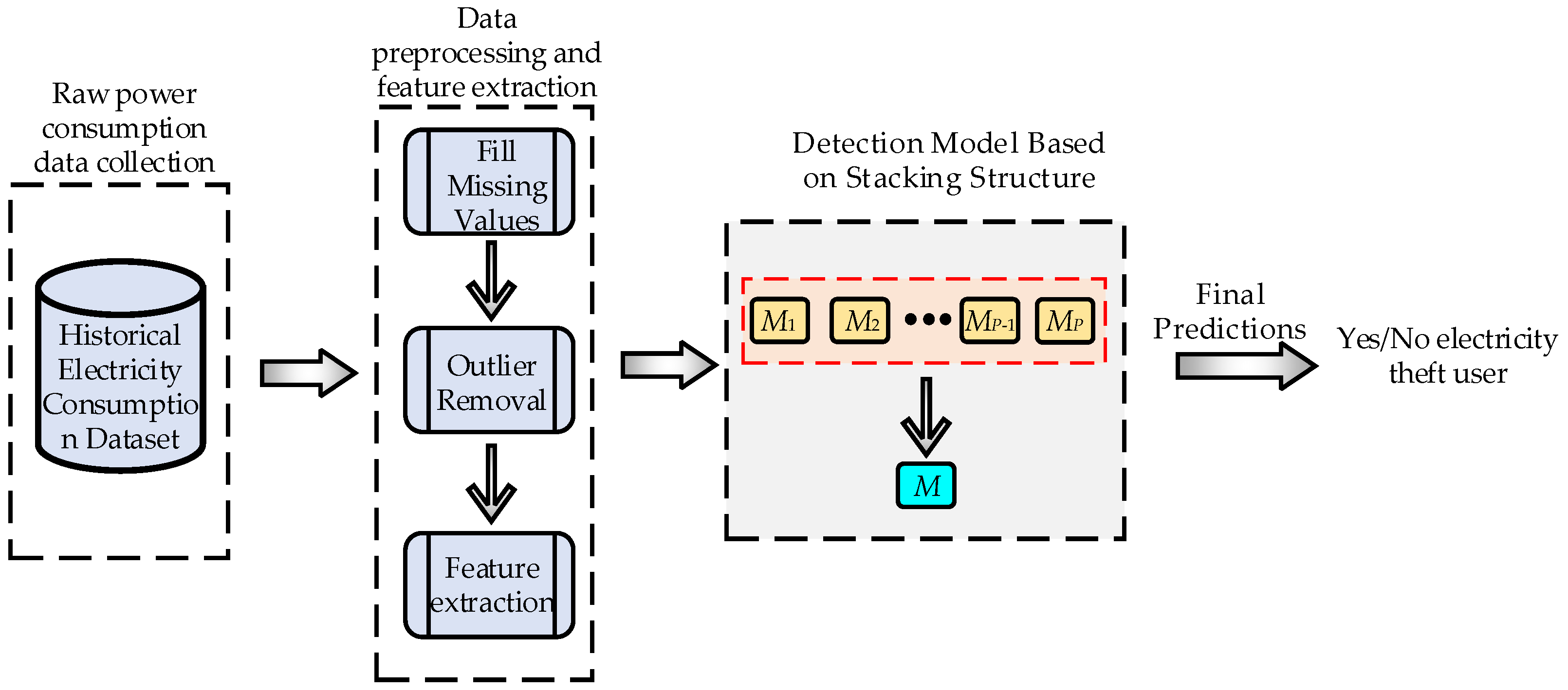
According to the experimental flow of the electricity theft detection model based on stacking structure in Figure 4, the data preprocessing, including missing value complement and outlier value repair, has been described in detail in Section 2 of the article, and the principle of feature extraction (i.e., load sequence feature extraction) for electricity consumption data has been described in detail in Section 2.3 of the article, where the load sequence feature extraction is performed on the SGCC dataset to obtain time series features [D₁,…, D₄₉]. The newly dimensionality-reducing features of the extracted high-dimensional time series [D₁,…, D₄₉] were then treated by the PCA method described above to obtain the new dimensionality-reducing feature values from largest to smallest: λ = [λ₁, λ₂, λ₃,…, λ₄₈, λ₄₉]. Calculate the value of l when the principal component contribution rate r ≥ 95% is calculated by Formula (10), and l = 6 is obtained after calculation, that is, the first six principal component eigenvalues are selected as the new feature set Y.

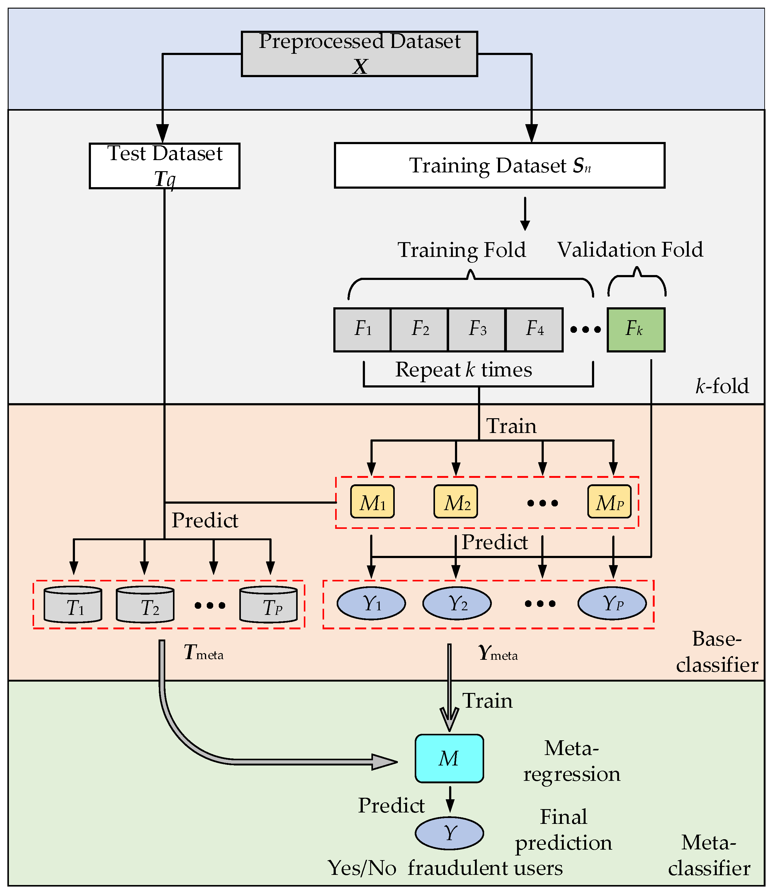
The selection of the base model layer and the metamodel layer in Figure 3 is the most important part of building the stacking structure, and the principle of the selection of the base model layer and the metamodel layer has been described in detail in Section 3.3, where the base model layer is more complex than the metamodel because of the large number of classifiers in this layer. The base model layer determines the weight values of a single performance index of the classifier by using a combined weight method of subjective weights and objective weights based on GRA, of which the subjective weight method obtains the weights of Recall, MAP@100, F₁-score and AUC through the AHP as shown in Table 4, and the weights of the four indicators are further calculated to be: w′ = (0.0598, 0.2933, 0.1786, 0.4683).

In order to obtain the objective weight w″ obtained by the EWM, the decision matrix R = (r_i,j)_m×n of each classifier or a combination of classifiers (that is, each scheme) is first required, that is, the different classifications in the stacking structure are selected. The combined base model has four performance indicators: Recall, MAP@100, F₁-score, and AUC under the new feature set Y after preprocessing, feature extraction and dimensionality reduction of the SGCC dataset, at this time, the meta-model of the stacking structure chooses a relatively simple linear regression (LR) model [38]. According to the classifier, selection of the base model layer, as in Section 3.3, should be strong and numerous, so the performance index values of eight existing classifiers commonly used for electricity theft detection under the new feature set Y are compared, and the eight classifiers are: random forest (RF) [39], eXtreme gradient boosting (XGBoost) [25], light gradient boosting machine (LightGBM) [40], support vector machine (SVM) [22], CART decision tree (DT) [23], deep forest (DF) [41], long short-term memory (LSTM) [28], and K-nearest neighbor (KNN) [42].

The hyperparameters of the above eight classifier algorithms are set to: In the RF model, the number of decision trees and the maximum depth of the tree are set to 101 and 15, respectively. The XGBoost model sets the learning rate to 0.5, the random sampling ratio to 0.08, and the maximum depth and optimal number of iterations to 3 and 10, respectively. The LightGBM model sets the number of leaf nodes to 10, the learning rate to 0.05, the feature selection scale and sample sampling ratio of the tree to 0.8, and the number of iterations required to perform bagging is 5. The SVM model sets the kernel function as a radial basis function, and the penalty coefficient C = 15. The DT model sets the confidence parameter θ = 0.25, the minimum number of instances on the leaf node ρ = 2. The number of decision trees required for the DF model to set up multi-granular scanning is K = 30, and the slicing window size is 15. The LSTM model sets the number of neurons to 32, the number of hidden layers to 2, the learning rate to 0.1, and the number of trees to 300. The KNN model sets the initial K value to 3.

The new feature set Y data samples are divided, and 50% of the data is randomly selected as the training sample (corresponding to 50% of the data as the test sample), and

Table 5. The experimental results of 8 classifiers under feature set Y.

Classifier	Metrics
	Recall	F1-Score	MAP@100	AUC
RF	0.87831	0.85061	0.86121	0.79187
XG	0.87483	0.84731	0.81756	0.78112
LG	0.86815	0.84441	0.81261	0.76108
SVM	0.86743	0.82417	0.76136	0.64407
DT	0.85911	0.79401	0.63899	0.63625
DF	0.72667	0.84617	0.82528	0.76551
LSTM	0.85928	0.83304	0.85928	0.76909
KNN	0.86001	0.79529	0.61371	0.64538

is the experimental results of the above eight classifiers, that is, the decision matrix R. Therefore, the objective weight method obtains call, MAP@100, F₁-score, and AUC through the EWM, and the four performance index weights are: w″ = (0.25899, 0.24321, 0.24851, 0.24929).

The combined weight vectors of each index of the combined weighting method can be obtained in three steps based on GRA: W_j = [0.0598, 0.2432, 0.2287, 0.4683]. According to the combined weight vector W_j, the comprehensive evaluation index values of the above eight classifiers are calculated: η₁ = [0.8273, 08107, 0.7991, 0.7318, 0.6863, 0.7962, 0.8110, 0.6848]^T, from which the comprehensive evaluation index of the above 8 classifiers is sorted as: RF > LSTM > XG > LG > DF > SVM > DT > KNN. The classifiers of the base model layer are combined according to the above eight classifiers, and the classifier combinations are combined from 2 to 8, where the number of combination types is: $C_8^2$+$C_8^3$+$C_8^4$+$C_8^5$+$C_8^6$+$C_8^7$+$C_8^8$ = 247, due to the many combinations, as shown in

Table 6. The experimental results of each classifier combination under feature set Y.

Number of Classifiers	The Combination of Classifiers	Metrics
		Recall	F1-Score	MAP@100	AUC
2	(DF + LSTM) ⅰ	0.89598	0.88095	0.92766	0.84267
	(XG + LSTM) ⅱ	0.90143	0.88937	0.94245	0.84268
	(LG + LSTM) ⅲ	0.90341	0.89259	0.95528	0.85764
3	(DF + LSTM + KNN) ⅳ	0.98431	0.91358	0.99378	0.94881
	(XG + LSTM + KNN) ⅴ	0.98642	0.98637	0.99872	0.95149
	(LG + LSTM + KNN) ⅵ	0.98712	0.99872	0.99969	0.97401
4	(DF + LSTM + KNN + SVM) ⅶ	0.98599	0.91531	0.99667	0.95691
	(XG + LSTM + KNN + SVM) ⅷ	0.98945	0.98431	0.99378	0.95841
	(LG + LSTM + KNN + SVM) ⅸ	0.98761	0.99898	0.99979	0.97659
5	(DF + LSTM + KNN + SVM + XG) ⅹ	0.97185	0.90857	0.98011	0.93027
6	(DF + LSTM + KNN + SVM + XG + LG) xi	0.96493	0.91571	0.97401	0.92857
7	(DF + LSTM + KNN + SVM + XG + LG + RF) xii	0.95944	0.91385	0.96815	0.92779
8	(DF + LSTM + KNN + SVM + XG + LG + RF + DT) xiii	0.94521	0.91706	0.96529	0.92262

.

The experimental results only list some valuable classifier combinations (each quantity combination classifier selects relatively good displays according to the performance index values) and its corresponding Recall, MAP@100, F₁-score, and AUC of the four performance index values. At this point, the meta-model of the stacking structure selects a linear regression model, and the k-fold setting k = 5.

The comprehensive evaluation index values of stacking structure integration learning method of each of the above classifier combinations were calculated by the combined weight vector W_j based on gray correlation degree analysis, and the results were: η₂ = [0.8746, 0.8804, 0.8912, 0.9526, 0.9729, 0.9867, 0.9576, 0.9746, 0.9879, 0.9389, 0.9380, 0.9355, 0.9324]^T. The η₂ corresponds to the comprehensive evaluation index values of each of the above classifier combinations, from which the comprehensive evaluation indexes of the above 13 classifier combinations can be sorted as follows: ix > vi > viii > v > vii > iv > x > xi > xii > xiii > iii > ii > i, that is, the top three combinations of the comprehensive evaluation index values of the 13 classifier combinations are: LG + LSTM + KNN + SVM, LG + LSTM + KNN and XG + LSTM + KNN + SVM, the corresponding comprehensive evaluation index values are 0.9879, 0.9867 and 0.9746, respectively. So, the stacking structure integration learning method of the three classifiers combination base model layers has a better effect on the detection and classification of electricity theft behavior.

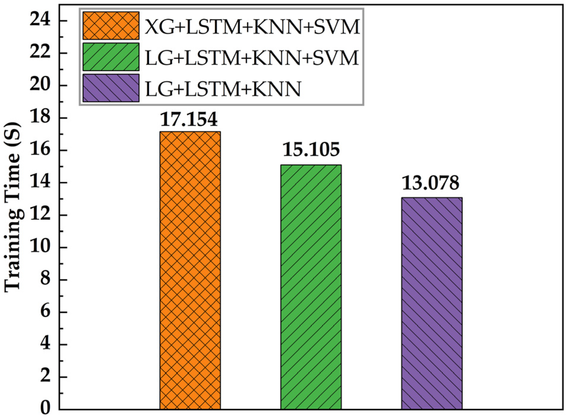
Through the above method, three classifier combinations with relatively good comprehensive evaluation index values were selected, but the comprehensive evaluation index values were relatively close (the difference was about 0.001). In order to select the optimal classifier combination, the training time of the model is also an important reference index for the real-time detection of electricity theft, so the training time of the stacking structure integration learning model under different classifier combinations is considered (at this time, the metamodel still uses a linear regression model). As shown in Figure 5, given the training time of the stacking structure integration learning model under different classifier combinations, it can be clearly concluded that when the base model layer adopts the LG + LSTM + KNN combination, the model training time of the stacking structure is the least, only 13.078 s. The longest model training time is the XG + LSTM + KNN + SVM combination, and the training time is 17.154 s.

Taking into account the accuracy of the model and the training time of the model, the base model layer of the stacking structure ensemble learning model selects LG + LSTM + KNN. The comprehensive evaluation index value of stacking structure ensemble learning model detection based on this base model layer is only 0.0012 different from the comprehensive evaluation index value of stacking structure ensemble learning model detection based on the combination of LG + LSTM + KNN + SVM. The training time difference is 2.027 s. Therefore, considering the above factors, the combination of LG + LSTM + KNN is selected as the base model of the stacking structure ensemble learning model.

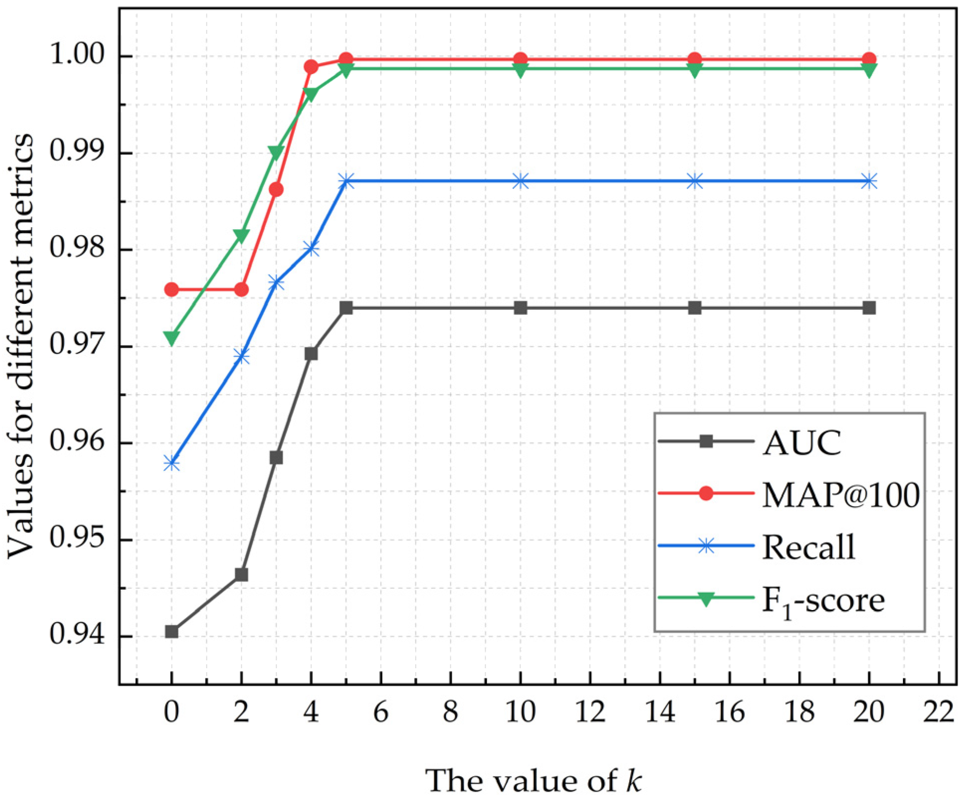
The above experiments set k = 5 in the k-fold layer, and different k values will greatly affect the detection effect of the stacking structure. According to the above experiments, the combination of LG + LSTM + KNN is selected as the base model of the stacking structure ensemble learning model, and the linear regression model is selected for the meta-model layer, and the k values are set to 2, 3, 4, 5, 10, 15, and 20 pairs of models respectively. After training, Figure 6 shows the experimental results under different k values, in which the experimental results are the four performance index values of Recall, MAP@100, F₁-score, and AUC. As can be seen from Figure 6, as the value of k increases, the values of the four performance indicators also increase. When the value of k is 5, each indicator value reaches the maximum value. On the other hand, the experimental results with k-fold cross-training are better than those without k-fold cross-training, so k-fold cross-training significantly improves the detection performance of the model. Therefore, when the combination of LG + LSTM + KNN constitutes a stacking structure, five-fold cross-training is selected, that is, k = 5 is set as the best parameter in the k-fold layer.

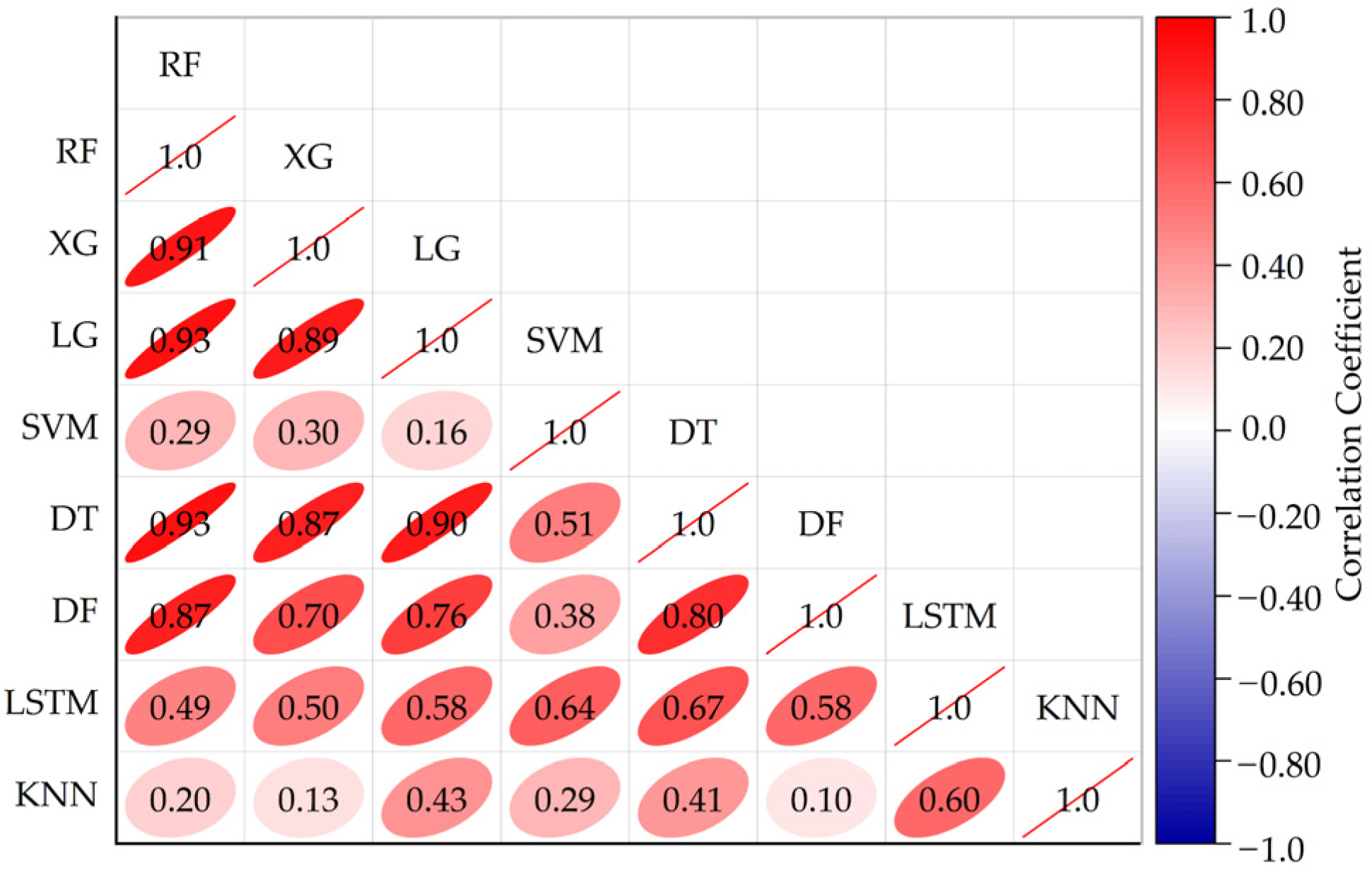
The stacking structure integration learning method integrates a variety of detection algorithms, which can make full use of each algorithm to observe data from different data spaces and structures. Therefore, the classifier of the base model layer should try to choose an algorithm with excellent performance and should also add different types or properties of classification algorithms as much as possible. In order to further verify and analyze the optimal base model combination selected, each base learner separately compares the classification prediction of the new feature set Y, and the Pearson correlation coefficient matrix is used to analyze the correlation of the classification prediction index values (AUC), and its calculation formula is as follows [33]:

$$r=\frac{{\displaystyle \sum _{i=1}^n(x_i-\overline{x})(y_i-\overline{y})}}{\sqrt{{\displaystyle \sum _{i=1}^n{(x_i-\overline{x})}^2{(y_i-\overline{y})}^2}}},$$

(23)

where $\overline{x},\overline{y}$ is the sample mean. The larger value of |r|, the more correlated it is. Figure 7 shows the correlation coefficient matrix between each classifier.

It can be seen from Figure 7 that the correlation degree of the value of the classification prediction index of each algorithm is generally high, which is due to the strong learning ability of each algorithm, and the inherent laws learned in the data during training are similar to the data observation angles. Among them, the classification prediction index values of RF, XG, LG, DF, and DT algorithms have the highest correlation, which is due to the fact that although the principles of the five types of algorithms are slightly different, they still belong to the integrated algorithms of the tree, and there are strong similarities in their data observation methods. The training mechanisms of LSTM, SVM, and KNN have a large gap, so the correlation of classification prediction index values is also low. Therefore, the effectiveness of the base model layer in choosing LG + LSTM + KNN algorithm combination as the base model in stacking integration learning is further verified.

4.2. Construction of Meta Model Layer in Stacking Structure

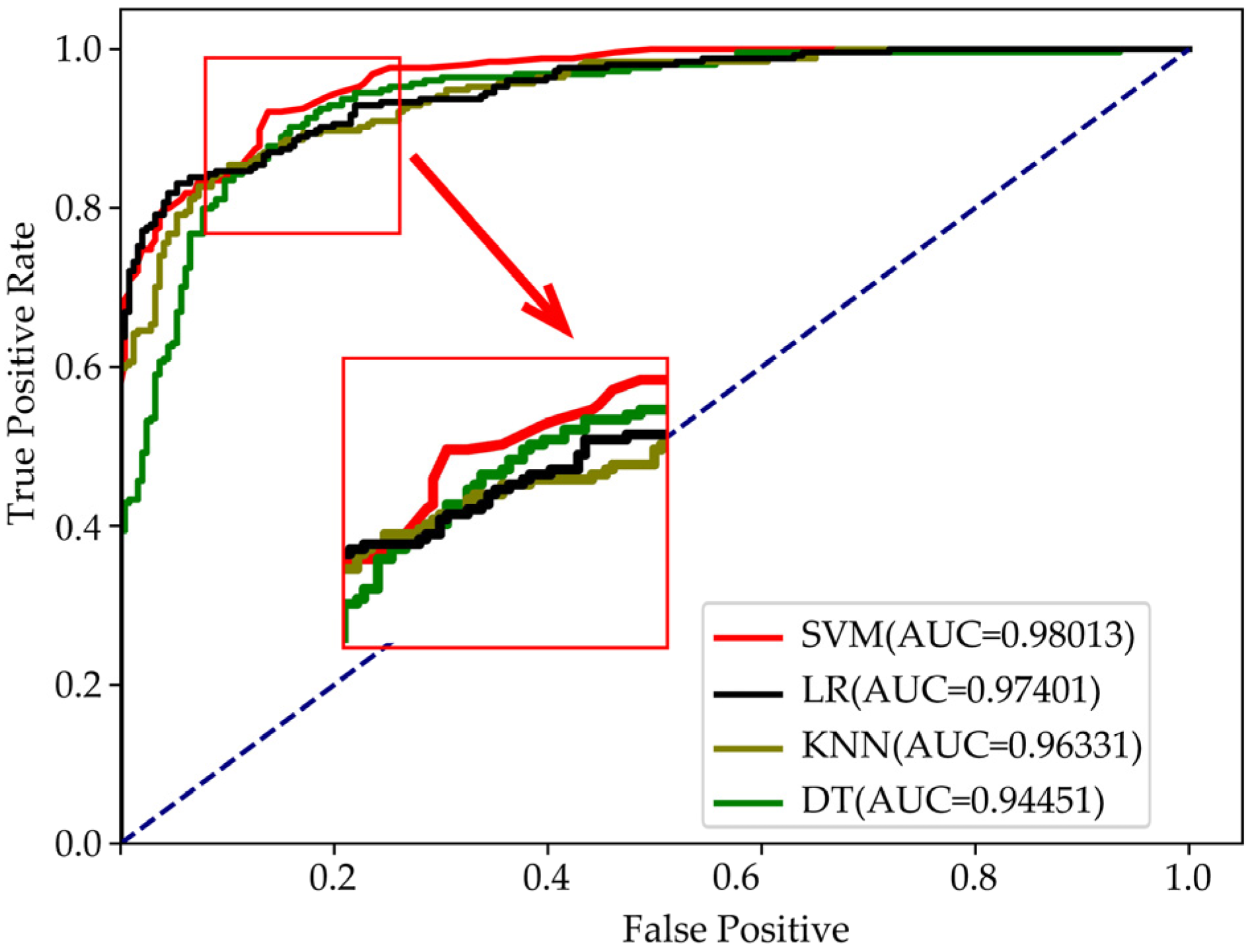
As described in Section 3.2, the meta-model layer usually chooses a relatively simple model to prevent the overfitting problem of the collation model, so this section selects several relatively simple models at the meta-classifier layer to compare the experimental results of the stacking structural integration learning method, including the SVM, DT, KNN, and LR. The ROC curves of the experimental results of the stacking structure under the above four different meta-models are shown in Figure 8.

It can be clearly seen from Figure 8 that when SVM is selected for the meta-model layer, the overall detection effect of Stacking ensemble learning is the best, and its AUC value is 0.98013. When the meta-model layer adopts decision tree, the sorting and detection effect of the stacking ensemble learning is slightly worse than the other three. Therefore, considering the detection effect, this paper adopts SVM as the model of the stacking integrated learning meta-model layer.

Since the recognition accuracy of the SVM algorithm is limited to a large extent by the selection of parameters, and the parameter optimization algorithm generally has problems, such as slow convergence speed and a tendency to fall into local extremums, the particle swarm optimization (PSO) algorithm [43] with strong optimization ability, fast convergence speed, and short calculation time is selected in this experiment to optimize the penalty coefficient C and kernel function (i.e., radial basis function) parameter σ values in the stacking integrated learning model metaclassifier SVM hyperparameter. 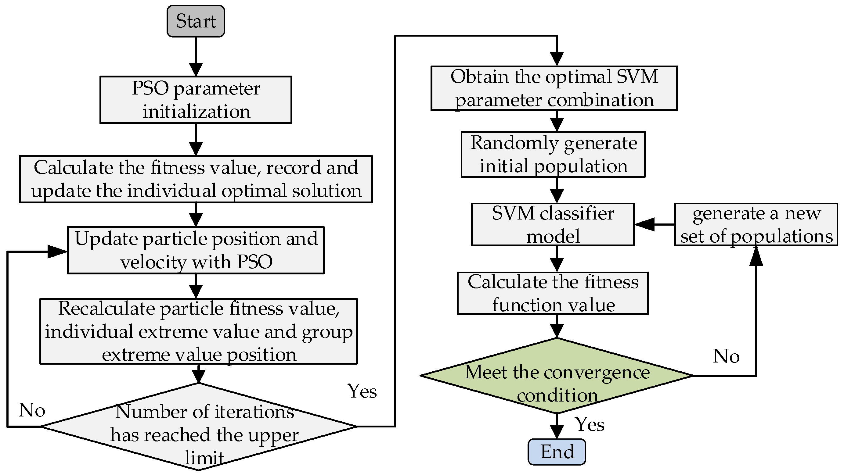Figure 9 shows the particle swarm optimization metaclassifier SVM hyperparameter flowchart, which is implemented as follows:

First of all, the initialization stage of the PSO parameter sets the step size and upper and lower boundaries of the search parameters, and the local optimal solution of the particles, the global optimal solution of the particle swarm, and its corresponding position are obtained by calculating the fitness function, and the fitness function adopts the cross-validation scores (CVS) method, which is calculated as follows [43]:

$$\mathrm{CVS}=\frac{1}{k}{\displaystyle \sum _{i=1}^k\frac{y_i}{y}},$$

(24)

where k is the number of cross-validations, y represents the number of training samples, y_i is the number of training samples that are correctly divided, and the higher the CVS value, the higher the accuracy of the model.

Second, the velocity and position of the individual particle swarm are iteratively updated according to the local optimal and global optimal solutions, and the cycle is reached until the maximum number of iterations is reached.

Finally, the parameters corresponding to the global optimal particle swarm individuals obtained above are trained as the initial parameters of the SVM, and the fitness value of each particle is calculated by the k-fold cross-validation value method again. If the adaptability of the new position is better than that of the local optimal particle, the local optimal particle is replaced with the new particle. If the optimal particle in the population is superior to the global optimal particle, the global optimal particle is replaced by the best particle in the population. The global optimal parameter C and σ values are returned after the above is completed.

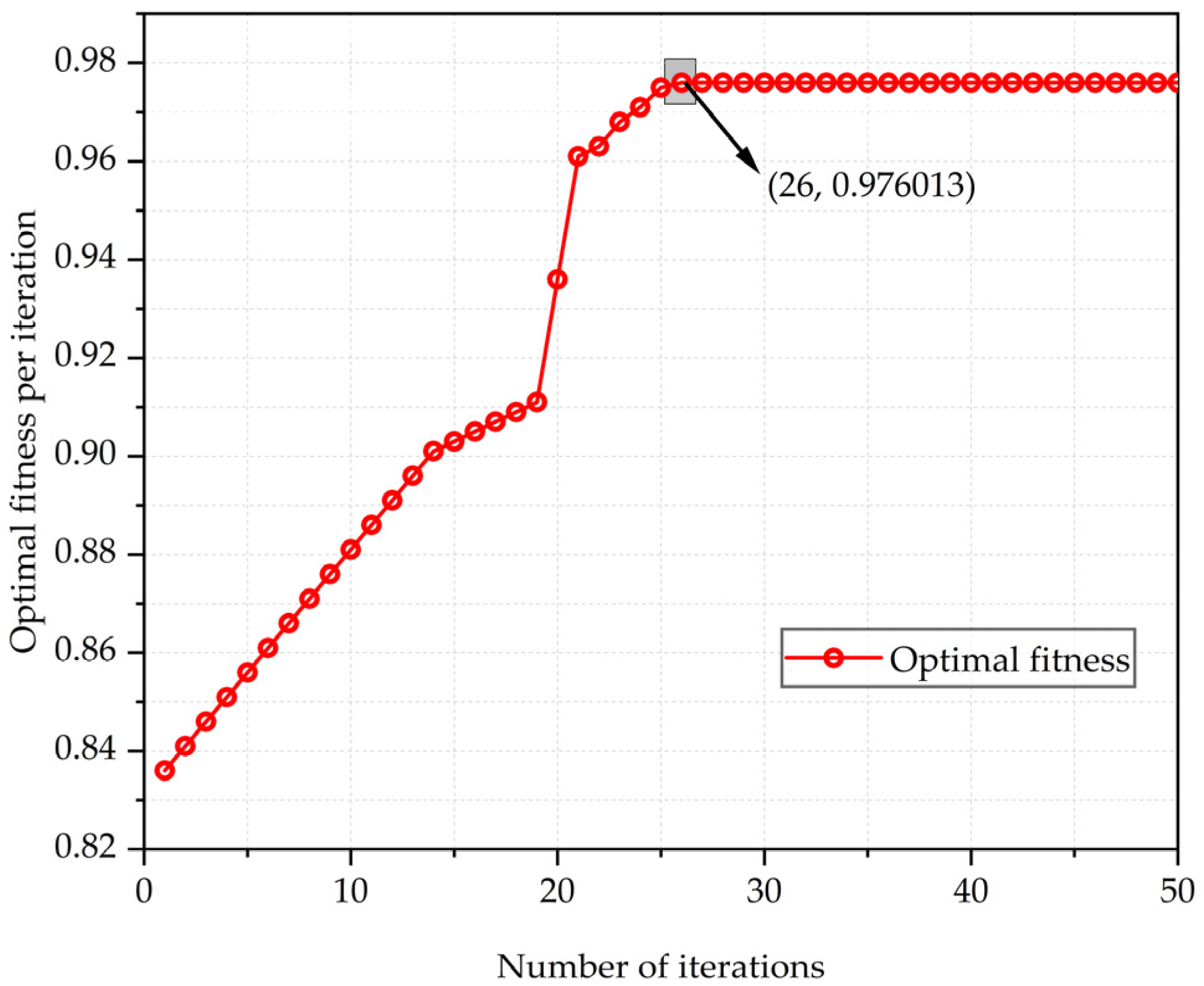
The above particle swarm algorithm optimizes the stacking ensemble learning model meta-classifier SVM hyperparameter, and the basic parameters of PSO setting are: acceleration factor c₁ and c₂ are both 2, inertia factor ω = 1, the number of particle swarms is 20, and the maximum number of iterations is 50. Figure 10 shows an evolutionary iteration plot that represents the resulting change in fitness values over different evolutionary algebras. As can be seen from Figure 10, PSO optimizes the SVM process, the fitness value remains unchanged after 26 iterations, and the final optimal fitness value is 0.976013, at which time the optimal parameter combination of the trained SVM is C = 21.375 and σ = 1.43.

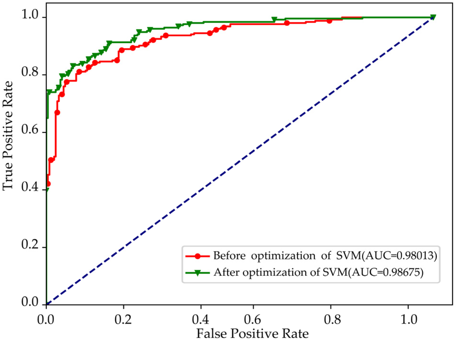
When the PSO optimization SVM obtains the best adaptability value, the AUC value is compared with the different effects before and after the optimization of the SVM parameters, as shown in Figure 11, which is the ROC curve of the stacking integration learning model before and after optimization.

It can be clearly seen from the ROC curve that the AUC value before optimization is 0.98013, while that after optimization is 0. 98675, and the AUC value is increased by about 0.007, because the detection effect of the stacking integrated learning model is relatively satisfactory, and the room for improvement is effective. So, SVM can relatively effectively improve the overall performance of the algorithm.

4.3. Comparison with Existing Methods

In order to verify the effectiveness of the detection method of stealing behavior based on the stacking ensemble learning model proposed in this paper, the experimental results are compared by using CNN [44], wide and deep CNN [27], hybrid deep neural networks (HDNNs) [45], CNN-RF [39] and the methods adopted in this paper. The dataset used in the above method is described in Section 3.1. Figure 12 shows the ROC curve of the above five methods, and the experimental results of the above five methods are shown in

Table 7. The methods proposed in this article compare the results with other methods.

Methods	Metrics
	Recall	F1-Score	MAP@100	AUC
CNN	0.82613	0.75625	0.86015	0.83447
wide and deep CNN	0.85862	0.86331	0.87329	0.84273
Hybrid Deep Neural Networks(HDNNs)	0.84228	0.86085	0.86265	0.83718
CNN-RF	0.87637	0.89628	0.91358	0.84729
The proposed method	0.98948	0.99913	0.99975	0.98675

.

We can see from Table 7 that the evaluation indicators of the method proposed in this paper under the actual power grid data are better than the other four existing detection methods, of which the AUC value is 0.98675, which is much higher than the other four methods.

In addition, for Recall and F₁-score, the method in this paper is one order of magnitude higher than other methods. For example, the Recall of this method reaches 0.98948, while the highest Recall value of the other four methods is CNN-RF, which is 0.87637. In addition, we found that the other four methods are all deep learning methods, three of which are variants of CNNs, that is, optimization on CNNs. Compared with the automatic extraction process of CNN, the purpose of manual feature extraction and selection of the proposed method is more clear and more efficient. Moreover, the stacking structure is a combination of multiple strong models that can learn from different angles of the data, and the learning ability of this method is stronger.

In summary, the evaluation indicators of CNN and its optimization methods have been improved to a certain extent, but they still cannot reach a very high level. It is worth noting that the method proposed in this paper can break through the bottleneck where other methods cannot improve after the accuracy reaches a certain level and achieve the purpose of improving the accuracy rate.

5. Conclusions

In this paper, we propose a multi-model fusion ensemble learning algorithm based on the stacking structure to detect electricity theft behaviors. The feature of this paper based on the stacking structure detection algorithm is that the PCA method is used to reduce the dimensionality of the user time series statistical feature indicators in the extracted dataset. That is, only the new properties of the first six principal component eigenvalues are used to ensure that a large amount of original information is not lost. The subjective weight values determined by the AHP method and the objective weight values determined by the EWM are combined and weighted by GRA method. The classifier combination of LG + LSTM + KNN with a relatively high comprehensive evaluation value (0.9867) and a relatively low model training time (13.078 s) is selected as the base model layer of the stacking structure by comprehensive evaluation index values through a large number of experiments.

In the meta-model layer, several relatively simple models are selected for comparative experiments. The SVM model with relatively good overall structure experimental results (the AUC value is 0.98013) of stacking is selected as the meta-model. The PSO algorithm is used to optimize the hyperparameters of the SVM model and improve the AUC value of the model from 0.98013 to 0.98675. By comparing the stacking structural model with the existing methods under the SGCC dataset, the effectiveness of the proposed methods is further verified. For example, the AUC value of the method proposed in this paper is 0.98675, which is an order of magnitude higher than the CNN-RF method with the highest AUC value of 0.84729 among other methods. Therefore, the stacking structure integrated learning method can effectively realize the accurate detection and identification of electricity theft behavior.

References

1. Xia, X.; Xiao, Y.; Liang, W.; Cui, J. Detection Methods in Smart Meters for Electricity Thefts: A Survey. Proc. IEEE 2022, 110, 273–319. [Google Scholar] [CrossRef]
2. Saeed, M.S.; Mustafa, M.W.; Hamadneh, N.N.; Alshammari, N.A.; Sheikh, U.U.; Jumani, T.A.; Khalid, S.B.A.; Khan, I. Detection of Non-Technical Losses in Power Utilities—A Comprehensive Systematic Review. Energies 2020, 13, 4727. [Google Scholar] [CrossRef]
3. Xia, X.; Xiao, Y.; Liang, W.; Zheng, M. GTHI: A Heuristic Algorithm to Detect Malicious Users in Smart Grids. IEEE Trans. Netw. Sci. Eng. 2020, 7, 805–816. [Google Scholar] [CrossRef]
4. Feng, X.; Hui, H.; Liang, Z.; Guo, W.; Que, H.; Feng, H.; Yao, Y.; Ye, C.; Ding, Y. A Novel Electricity Theft Detection Scheme Based on Text Convolutional Neural Networks. Energies 2020, 13, 5758. [Google Scholar] [CrossRef]
5. Park, C.H.; Kim, T. Energy Theft Detection in Advanced Metering Infrastructure Based on Anomaly Pattern Detection. Energies 2020, 13, 3832. [Google Scholar] [CrossRef]
6. Xiong, D.; Chen, Y.; Chen, X.; Liu, X.; Yang, M. Design and Application of Intelligent Electricity Monitoring Device. In Proceedings of the 2018 International Conference on Power System Technology (POWERCON), Guangzhou, China, 6–8 November 2018; pp. 3312–3317. [Google Scholar]
7. Pamir; Javaid, N.; Javaid, S.; Asif, M.; Javed, M.U.; Yahaya, A.S.; Aslam, S. Synthetic Theft Attacks and Long Short Term Memory-Based Preprocessing for Electricity Theft Detection Using Gated Recurrent Unit. Energies 2022, 15, 2778. [Google Scholar] [CrossRef]
8. Raggi, L.M.; Trindade, F.C.; Cunha, V.C.; Freitas, W. Non-Technical Loss Identification by Using Data Analytics and Customer Smart Meters. IEEE Trans. Power Del. 2020, 35, 2700–2710. [Google Scholar] [CrossRef]
9. Leite, J.B.; Mantovani, J.R.S. Detecting and Locating Non-Technical Losses in Modern Distribution Networks. IEEE Trans. Smart Grid 2018, 9, 1023–1032. [Google Scholar] [CrossRef] [Green Version]
10. Zanetti, M.; Jamhour, E.; Pellenz, M.; Penna, M.; Zambenedetti, V.; Chueiri, I. A Tunable Fraud Detection System for Advanced Metering Infrastructure Using Short-Lived Patterns. IEEE Trans. Smart Grid 2019, 10, 830–840. [Google Scholar] [CrossRef]
11. Guerrero, J.I.; Monedero, I.; Biscarri, F.; Biscarri, J.; Millan, R.; Leon, C. Non-Technical Losses Reduction by Improving the Inspections Accuracy in a Power Utility. IEEE Trans. Power Syst. 2018, 33, 1209–1218. [Google Scholar] [CrossRef]
12. Wei, L.; Sundararajan, A.; Sarwat, A.I.; Biswas, S.E.; Ibrahim, E. A distributed intelligent framework for electricity theft detection using benford’s law and stackelberg game. In Proceedings of the 2017 Resilience Week (RWS), Wilmington, DE, USA, 18–22 September 2017; pp. 5–11. [Google Scholar]
13. Chen, Q.; Zheng, K.; Kang, C.; Huang, F. Detection Methods of Abnormal Electricity Consumption Behaviors: Review and Prospect. Autom. Electr. Power Syst. 2018, 42, 189–199. [Google Scholar]
14. Amin, S.; Schwartz, G.A.; Cardenas, A.A.; Sastry, S.S. Game-Theoretic Models of Electricity Theft Detection in Smart Utility Networks: Providing New Capabilities with Advanced Metering Infrastructure. IEEE Control Syst. Mag. 2015, 35, 66–81. [Google Scholar]
15. Gao, Y.; Foggo, B.; Yu, N. A Physically Inspired Data-Driven Model for Electricity Theft Detection With Smart Meter Data. IEEE Trans. Ind. Informat. 2019, 15, 5076–5088. [Google Scholar] [CrossRef]
16. Zheng, K.; Chen, Q.; Wang, Y.; Kang, C.; Xia, Q. A Novel Combined Data-Driven Approach for Electricity Theft Detection. IEEE Trans. Ind. Informat. 2019, 15, 1809–1819. [Google Scholar] [CrossRef]
17. Takiddin, A.; Ismail, M.; Zafar, U.; Serpedin, E. Robust Electricity Theft Detection Against Data Poisoning Attacks in Smart Grids. IEEE Trans. Smart Grid 2021, 12, 2675–2684. [Google Scholar] [CrossRef]
18. Zhang, Q.; Zhang, M.; Chen, T.; Fan, J.; Yang, Z.; Li, G. Electricity Theft Detection Using Generative Models. In Proceedings of the 2018 IEEE 30th International Conference on Tools with Artificial Intelligence (ICTAI), Volos, Greece, 5–7 November 2018; pp. 270–274. [Google Scholar]
19. Aslam, Z.; Ahmed, F.; Almogren, A.; Shafiq, M.; Zuair, M.; Javaid, N. An Attention Guided Semi-Supervised Learning Mechanism to Detect Electricity Frauds in the Distribution Systems. IEEE Access 2020, 8, 221767–221782. [Google Scholar] [CrossRef]
20. Lu, X.; Zhou, Y.; Wang, Z.; Yi, Y.; Feng, L.; Wang, F. Knowledge Embedded Semi-Supervised Deep Learning for Detecting Non-Technical Losses in the Smart Grid. Energies 2019, 12, 3452. [Google Scholar] [CrossRef] [Green Version]
21. Li, J.; Wang, F. Non-Technical Loss Detection in Power Grids with Statistical Profile Images Based on Semi-Supervised Learning. Sensors 2020, 20, 236. [Google Scholar] [CrossRef] [Green Version]
22. Wu, R.; Wang, L.; Hu, T. AdaBoost-SVM for Electrical Theft Detection and GRNN for Stealing Time Periods Identification. In Proceedings of the IECON 2018-44th Annual Conference of the IEEE Industrial Electronics Society, Washington, DC, USA, 21–23 October 2018; pp. 3073–3078. [Google Scholar]
23. Kong, X.; Zhao, X.; Liu, C.; Li, Q.; Li, Y. Electricity theft detection in low-voltage stations based on similarity measure and dt-ksvm. Int. J. Electr. Power Energy Syst. 2021, 125, 106544. [Google Scholar] [CrossRef]
24. Buzau, M.M.; Tejedor-Aguilera, J.; Cruz-Romero, P.; Gómez-Expósito, A. Detection of Non-Technical Losses Using Smart Meter Data and Supervised Learning. IEEE Trans. Smart Grid 2019, 10, 2661–2670. [Google Scholar] [CrossRef]
25. Yan, Z.; Wen, H. Electricity Theft Detection Base on Extreme Gradient Boosting in AMI. IEEE Trans. Instrum. Meas. 2021, 70, 1–9. [Google Scholar] [CrossRef]
26. Razavi, R.; Gharipour, A.; Fleury, M.; Justice, A.I. A practical feature-engineering framework for electricity theft detection in smart grids. Appl. Energy 2019, 238, 481–494. [Google Scholar] [CrossRef]
27. Zheng, Z.; Yang, Y.; Niu, X.; Dai, H.-N.; Zhou, Y. Wide and Deep Convolutional Neural Networks for Electricity-Theft Detection to Secure Smart Grids. IEEE Trans. Ind. Informat. 2018, 14, 1606–1615. [Google Scholar] [CrossRef]
28. Hasan, M.N.; Toma, R.N.; Nahid, A.-A.; Islam, M.M.M.; Kim, J.-M. Electricity Theft Detection in Smart Grid Systems: A CNN-LSTM Based Approach. Energies 2019, 12, 3310. [Google Scholar] [CrossRef] [Green Version]
29. Zhai, D.; Pan, Y.; Li, P.; Li, G. Estimating the Vigilance of High-Speed Rail Drivers Using a Stacking Ensemble Learning Method. IEEE Sensors J. 2021, 21, 16826–16838. [Google Scholar] [CrossRef]
30. Tang, Y.; Gu, L.; Wang, L. Deep Stacking Network for Intrusion Detection. Sensors 2022, 22, 25. [Google Scholar] [CrossRef]
31. Zhao, R.; Mu, Y.; Zou, L.; Wen, X. A Hybrid Intrusion Detection System Based on Feature Selection and Weighted Stacking Classifier. IEEE Access 2022, 10, 71414–71426. [Google Scholar] [CrossRef]
32. Tan, R.; Zhang, W.; Chen, S. Decision-Making Method Based on Grey Relation Analysis and Trapezoidal Fuzzy Neutrosophic Numbers Under Double Incomplete Information and its Application in Typhoon Disaster Assessment. IEEE Access 2020, 8, 3606–3628. [Google Scholar] [CrossRef]
33. Takiddin, A.; Ismail, M.; Nabil, M.; Mahmoud, M.M.; Serpedin, E. Detecting Electricity Theft Cyber-Attacks in AMI Networks Using Deep Vector Embeddings. IEEE Syst. J. 2021, 15, 4189–4198. [Google Scholar] [CrossRef]
34. Seghouane, A.-K.; Shokouhi, N.; Koch, I. Sparse Principal Component Analysis with Preserved Sparsity Pattern. IEEE Trans. Image Process. 2019, 28, 3274–3285. [Google Scholar] [CrossRef]
35. Pavlyshenko, B. Using Stacking Approaches for Machine Learning Models. In Proceedings of the 2018 IEEE Second International Conference on Data Stream Mining & Processing (DSMP), Lviv, Ukraine, 21–25 August 2018; pp. 255–258. [Google Scholar]
36. Wang, X. Design and Implementation of College English Teaching Quality Evaluation System Based on Analytic Hierarchy Process. In Proceedings of the 2020 International Conference on Computers, Information Processing and Advanced Education (CIPAE), Ottawa, Canada, 16–18 October 2020; pp. 213–216. [Google Scholar]
37. Yin, J.; Han, L.; Ma, L.; Cai, H.; Li, H.; Li, J.; Sun, G. Evaluation of Terminal Signal Quality based on Entropy Weight Method. In Proceedings of the 2022 4th International Conference on Intelligent Control, Measurement and Signal Processing (ICMSP), Hangzhou, China, 8–10 July 2022; pp. 855–858. [Google Scholar]
38. Adeli, E.; Li, X.; Kwon, D.; Zhang, Y.; Pohl, K.M. Logistic Regression Confined by Cardinality-Constrained Sample and Feature Selection. IEEE Trans. Pattern Anal. Mach. Intell. 2020, 42, 1713–1728. [Google Scholar] [CrossRef] [PubMed] [Green Version]
39. Shuan, L.; Ying, H.; Xu, Y.; Ying, S.; Jin, W.; Qiang, Z. Electricity Theft Detection in Power Grids with Deep Learning and Random Forests. J. Electr. Comput. Eng. 2019, 2019, 1–12. [Google Scholar] [CrossRef]
40. Tang, M.; Zhao, Q.; Ding, S.X.; Wu, H.; Li, L.; Long, W.; Huang, B. An Improved LightGBM Algorithm for Online Fault Detection of Wind Turbine Gearboxes. Energies 2020, 13, 807. [Google Scholar] [CrossRef] [Green Version]
41. Xie, R.; Cui, Z.; Jia, M.; Wen, Y.; Hao, B. Testing Coverage Criteria for Deep Forests. In Proceedings of the 2019 6th International Conference on Dependable Systems and Their Applications (DSA), Harbin, China, 3–6 January 2020; pp. 513–514. [Google Scholar]
42. Vieira, J.; Duarte, R.P.; Neto, H.C. kNN-STUFF: kNN STreaming Unit for Fpgas. IEEE Access 2019, 7, 170864–170877. [Google Scholar] [CrossRef]
43. Wu, Y.; Liu, Y.; Li, N.; Wang, S. Hybrid Multi-objective Particle Swarm Optimization Algorithm Based on Particle Sorting. In Proceedings of the 2021 IEEE International Conference on Emergency Science and Information Technology (ICESIT), Chongqing, China, 22–24 November 2021; pp. 257–260. [Google Scholar]
44. Yao, D.; Wen, M.; Liang, X.; Fu, Z.; Zhang, K.; Yang, B. Energy Theft Detection with Energy Privacy Preservation in the Smart Grid. IEEE Internet Things J. 2019, 6, 7659–7669. [Google Scholar] [CrossRef]
45. Buzau, M.; Tejedor-Aguilera, J.; Cruz-Romero, P.; Gómez-Expósito, A. Hybrid Deep Neural Networks for Detection of Non-Technical Losses in Electricity Smart Meters. IEEE Trans. Power Syst. 2020, 35, 1254–1263. [Google Scholar] [CrossRef]
Figure 1. Three types of physical electricity theft methods. (a) Voltage reduction type wiring diagram. (b) Current reducing type wiring diagram. (c.1) Power factor reduction type wiring diagram. (c.2) Power factor reduction type phase diagram.
Energies 15 07423 g001
Figure 2. The usual structure of ensemble learning.
Energies 15 07423 g002
Figure 3. Structure of stacking integrated model.
Energies 15 07423 g003
Figure 4. Structure of stacking integrated model experimental flow chart.
Energies 15 07423 g004
Figure 5. Training time of stacking structure integration learning model under different classifier combinations.
Energies 15 07423 g005
Figure 6. Experimental results of stacking structure with different k values.
Energies 15 07423 g006
Figure 7. Matrix of correlation coefficients for the value of the classification prediction indicator between classifiers.
Energies 15 07423 g007
Figure 8. The ROC curve of stacking structures under different meta-models.
Energies 15 07423 g008
Figure 9. Flowchart of PSO to optimize meta-classifier (SVM) hyperparameters.
Energies 15 07423 g009
Figure 10. Diagram of evolutionary iterations.
Energies 15 07423 g010
Figure 11. ROC curve before and after optimization.
Energies 15 07423 g011
Figure 12. The ROC curves of the method proposed in this paper and the other four methods.
Energies 15 07423 g012