
Thermochemical Properties for Valorization of Amazonian Biomass as Fuel

 , , ,
, , ,  , , and
Abstract
: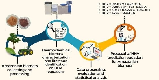
1. Introduction

| Equation | Source | HHV Equation (MJ/kg) wt. %, Dry Basis | Biomass Data Origin | Type of Analysis |
|---|---|---|---|---|
| (1) | [23] | HHV = −1.6701 + 0.4373 × C | Wood from different countries | Ultimate |
| (2) | [21] | HHV = −0.763 + 0.301 × C + 0.525 × H + 0.064 × O | Field crop residues, orchard pruning, vineyard pruning, food and fiber processing wastes, forest residues and energy crops from California | Ultimate |
| (3) | [15] | HHV = −10.81408 + 0.3133 × (V + FC) | Agricultural residues from Spain | Proximate |
| (4) | [5] | HHV = 35.43 − 0.1835 × V − 0.3543 × A | Forest and agricultural wastes/chars from Spain and Cuba | Proximate |
| (5) | [16] | HHV = 0.1534 × V + 0.312 × FC | Turkey | Proximate |
| (6) | [19] | HHV = −1.3675 + 0.3237 × C + 0.7009 × H + 0.0318 × O | Various types from the open literature | Ultimate |
| (7) | [19] | HHV = 3.4597 + 0.3259 × C | Various types from the open literature | Ultimate |
| (8) | [19] | HHV = −3.0368 + 0.2218 × V + 0.26 × FC | Various types from the open literature | Proximate |
| (9) | [22] | HHV = 0.3491 × C + 1.1783 × H + 0.1005 × S − 0.1034 × O − 0.0151 × N − 0.0211 × A | Gases, liquids, solid fuels (coal/coke), wood, sawdust, refuse, MSW, animal waste from the open literature | Ultimate |
| (10) | [13] | HHV = 0.3536 × FC + 0.1559 × V − 0.0078 × A | Fuels such as coals/lignite/manufactured fuel/all kinds of biomass/industry waste from the open literature | Proximate |
| (11) | [20] | HHV = 0.3560 + 0.4328 × C − 0.2977 × H + 0.2874 × N | Straw from China | Ultimate |
| (12) | [17] | HHV = 0.1905 × V + 0.2521 × FC | Agricultural byproducts/wood from Argentina, Australia, Cuba, Greece, India, Morocco, the Netherlands, Spain, Turkey and the United States of America | Proximate |
| (13) | [17] | HHV = 0.2949 × C + 0.8250 × H | Agricultural byproducts/wood from Argentina, Australia, Cuba, Greece, India, Morocco, the Netherlands, Spain, Turkey and the United States of America | Ultimate |
| (14) | [26] | HHV = −3.393 + 0.507 × C − 0.341 × H + 0.067 × N | Crop species from Spain | Ultimate |
| (15) | [26] | HHV = −13.173 + 0.416 × V | Crop species from Spain | Proximate |
| (16) | [14] | HHV = 19.2880 − 0.2135 × (V/FC) − 1.9584 × (A/V) + 0.0234 × (FC/A) | Various types from the open literature | Proximate |
| (17) | [12] | HHV = 0.879 × C + 0.321 × H + 0.056 × O − 24.826 | Oil palm fronds from Malaysia | Ultimate |
| (18) | [24] | HHV = 0.4373 × C − 1.6701 | Agroforestry biomass from Russia | Ultimate |
| (19) | [27] | HHV = 0.2328 × C + 6.9703 | Various types from the open literature | Ultimate |
| (20) | [18] | HHV = −0.0038 × (−19.9812 × FC1.2259) + (−1.0298 × 10⁻¹³ × V × 8.0664) + (0.1026 × A2.423) + (−1.2065 × 10⁻⁷ × FC × A4.6653 + 0.0228 × FC × V × A) + (−0.2511 × (V/A) − (0.0478 × (FC/V)) + 15.7199 | Various types from the open literature | Proximate |
| (21) | [28] | HHV = 0.3826 × C − 0.3681 × H + 2.7882 × S − 0.0378 × O + 0.9262 | Biomass/biochar from Malaysia | Ultimate |
2. Materials and Methods
2.1. Biomass Characteristics
2.2. Development of Regression Equations
2.2.1. Pearson’s Correlation
2.2.2. Linear Regression Methods
2.2.3. Statistical Analysis
R2 and R2-Adjusted
F-Test and p-Value
Error Analysis
- Mean absolute error (MAE);
- Mean absolute percentage of error (MAPE);
- Square root of mean error (SRME).
2.3. Validation Databank
2.4. HHV Equations from the Literature: Models Used for Comparison
3. Results and Discussion
3.1. Biomass Characteristics
3.2. Development of the Models for the HHV
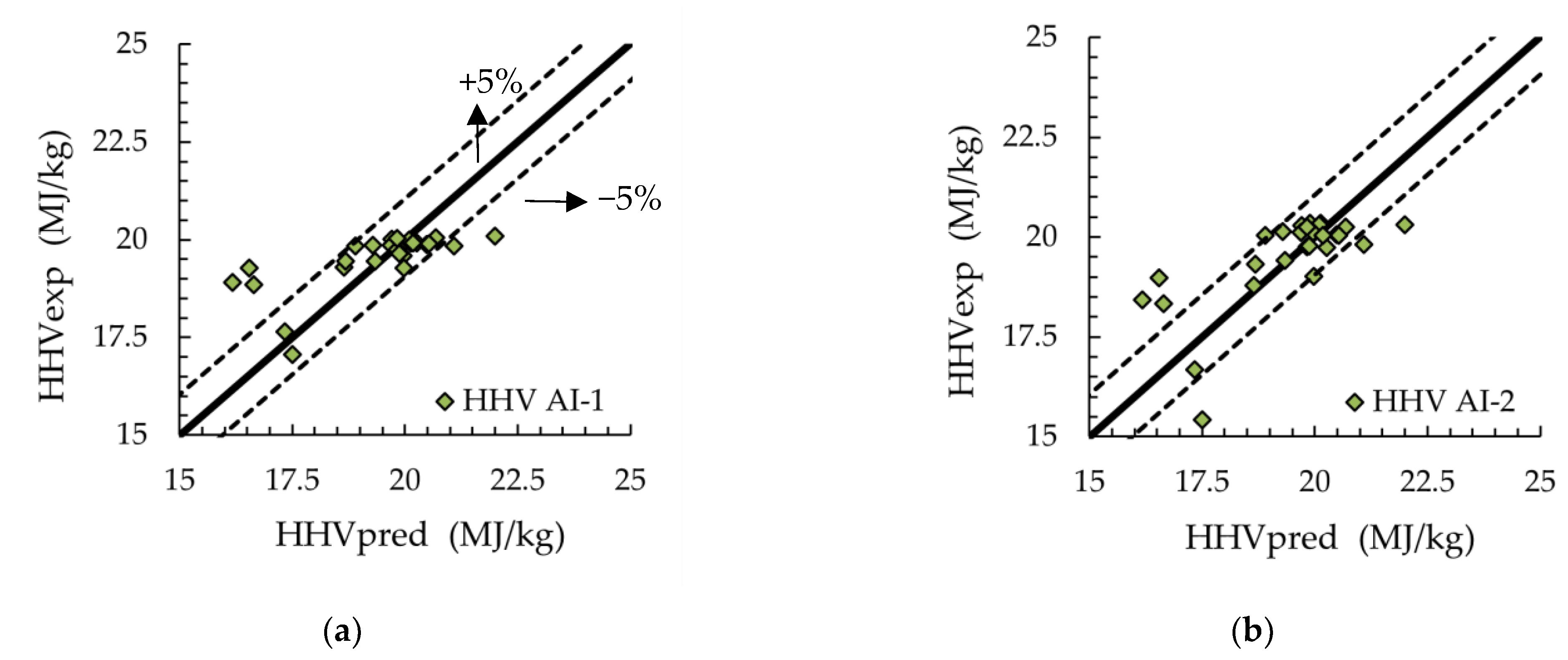
3.3. Validation of the Proposed HHV Equations
3.4. Results of the Comparison between the Proposed and Literature Equations
4. Conclusions
Author Contributions
Funding
Data Availability Statement
Acknowledgments
Conflicts of Interest
References
- Empresa de Pesquisa Energética (Brasil). Brazilian Energy Balance 2021 Year 2020; Empresa de Pesquisa Energética (Brasil): Brasilia, Brazil, 2021; p. 292.
- Chavando, J.A.M.; Silva, V.; Guerra, D.R.D.S.; Eusébio, D.; Cardoso, J.S.; Tarelho, L.A. Review Chapter: Waste to Energy through Pyrolysis and Gasification in Brazil and Mexico. In Gasification; Intech Open: London, UK, 2021. [Google Scholar] [CrossRef]
- Araujo, R.O.; Ribeiro, F.C.P.; Santos, V.O.; Lima, V.M.R.; Santos, J.L.; Vilaça, J.E.S.; Chaar, J.S.; Falcão, N.P.S.; Pohlit, A.M.; de Souza, L.K.C. Renewable Energy from Biomass: An Overview of the Amazon Region. Bioenergy Res. 2022, 15, 834–849. [Google Scholar] [CrossRef]
- van Loo, S.; Koppejan, J. The Handbook of Biomass Combustion and Co-Firing; Earthscan: London, UK, 2008. [Google Scholar]
- Cordero, T.; Marquez, F.; Rodriguez-Mirasol, J.; Rodriguez, J. Predicting heating values of lignocellulosics and carbonaceous materials from proximate analysis. Fuel 2001, 80, 1567–1571. [Google Scholar] [CrossRef]
- Qian, H.; Guo, X.; Fan, S.; Hagos, K.; Lu, X.; Liu, C.; Huang, D. A Simple Prediction Model for Higher Heat Value of Biomass. J. Chem. Eng. Data 2016, 61, 4039–4045. [Google Scholar] [CrossRef]
- Hasan, M.; Haseli, Y.; Karadogan, E. Correlations to Predict Elemental Compositions and Heating Value of Torrefied Biomass. Energies 2018, 11, 2443. [Google Scholar] [CrossRef] [Green Version]
- Dai, Z.; Chen, Z.; Selmi, A.; Jermsittiparsert, K.; Denić, N.M.; Nešić, Z. Machine learning prediction of higher heating value of biomass. Biomass Convers. Biorefin. 2021, 1–9. [Google Scholar] [CrossRef]
- Wahid, F.R.A.A.; Saleh, S.; Samad, N.A.F.A. Estimation of Higher Heating Value of Torrefied Palm Oil Wastes from Proximate Analysis. Energy Procedia 2017, 138, 307–312. [Google Scholar] [CrossRef] [Green Version]
- Keybondorian, E.; Zanbouri, H.; Bemani, A.; Hamule, T. Estimation of the higher heating value of biomass using proximate analysis. Energy Sources Part A Recover. Util. Environ. Eff. 2017, 39, 2025–2030. [Google Scholar] [CrossRef]
- Akkaya, A.V. Proximate analysis based multiple regression models for higher heating value estimation of low rank coals. Fuel Process. Technol. 2009, 90, 165–170. [Google Scholar] [CrossRef]
- Elneel, R.; Anwar, S.; Ariwahjoed, B. Prediction of Heating Values of Oil Palm Fronds from Ultimate Analysis. J. Appl. Sci. 2013, 13, 491–496. [Google Scholar] [CrossRef]
- Parikh, J.; Channiwala, S.A.; Ghosal, G.K. A Correlation for Calculating HHV from Proximate Analysis of Solid Fuels. Fuel 2005, 84, 487–494. [Google Scholar] [CrossRef]
- Nhuchhen, D.R.; Salam, P.A. Estimation of higher heating value of biomass from proximate analysis: A new approach. Fuel 2012, 99, 55–63. [Google Scholar] [CrossRef]
- Jiménez, L.; Gonzalez, F. Study of the physical and chemical properties of lignocellulosic residues with a view to the production of fuels. Fuel 1991, 70, 947–950. [Google Scholar] [CrossRef]
- Demirbaş, A. Calculation of higher heating values of biomass fuels. Fuel 1997, 76, 431–434. [Google Scholar] [CrossRef]
- Yin, C.-Y. Prediction of higher heating values of biomass from proximate and ultimate analyses. Fuel 2011, 90, 1128–1132. [Google Scholar] [CrossRef] [Green Version]
- Dashti, A.; Noushabadi, A.S.; Raji, M.; Razmi, A.; Ceylan, S.; Mohammadi, A.H. Estimation of biomass higher heating value (HHV) based on the proximate analysis: Smart modeling and correlation. Fuel 2019, 257, 115931. [Google Scholar] [CrossRef]
- Sheng, C.; Azevedo, J. Estimating the higher heating value of biomass fuels from basic analysis data. Biomass Bioenergy 2005, 28, 499–507. [Google Scholar] [CrossRef]
- Huang, C.; Han, L.; Yang, Z.; Liu, X. Ultimate analysis and heating value prediction of straw by near infrared spectroscopy. Waste Manag. 2009, 29, 1793–1797. [Google Scholar] [CrossRef]
- Jenkins, B.M.; Ebeling, J.M. Thermochemical Properties of Biomass Fuels. Calif. Agric. 1985, 39, 14–16. [Google Scholar]
- Channiwala, S.; Parikh, P. A unified correlation for estimating HHV of solid, liquid and gaseous fuels. Fuel 2002, 81, 1051–1063. [Google Scholar] [CrossRef]
- Tillman, D.A. Wood as an Energy Resource; Academic Press: New York, NY, USA, 1978; ISBN 9780126912609. [Google Scholar]
- Bychkov, A.L.; Denkin, A.I.; Tikhova, V.; Lomovsky, O. Prediction of higher heating values of plant biomass from ultimate analysis data. J. Therm. Anal. Calorim. 2017, 130, 1399–1405. [Google Scholar] [CrossRef]
- Ahmed, A.; Bakar, M.; Razzaq, A.; Hidayat, S.; Jamil, F.; Amin, M.; Sukri, R.; Shah, N.; Park, Y.-K. Characterization and Thermal Behavior Study of Biomass from Invasive Acacia mangium Species in Brunei Preceding Thermochemical Conversion. Sustainability 2021, 13, 5249. [Google Scholar] [CrossRef]
- Callejón-Ferre, A.; Velázquez-Martí, B.; López-Martínez, J.; Manzano-Agugliaro, F. Greenhouse crop residues: Energy potential and models for the prediction of their higher heating value. Renew. Sustain. Energy Rev. 2011, 15, 948–955. [Google Scholar] [CrossRef]
- Boumanchar, I.; Charafeddine, K.; Chhiti, Y.; Alaoui, F.E.M.; Sahibed-Dine, A.; Bentiss, F.; Jama, C.; Bensitel, M. Biomass higher heating value prediction from ultimate analysis using multiple regression and genetic programming. Biomass Convers. Biorefin. 2019, 9, 499–509. [Google Scholar] [CrossRef]
- Afiqah, N.; Kamaruddin, B.; Azlina, W.; Abdul, W.; Ghani, K.; Rezi, M.; Hamid, A.; Alias, A.B.; Shamsudin, A.H. Simulation and Analysis of Calorific Value for Biomass Solid Waste as a Potential Solid Fuel Source for Power Generation. Jase. Tku. Edu. Tw 2022, 26, 163–173. [Google Scholar]
- Lopes, F.C.R.; Pereira, J.C.; Tannous, K. Thermal decomposition kinetics of guarana seed residue through thermogravimetric analysis under inert and oxidizing atmospheres. Bioresour. Technol. 2018, 270, 294–302. [Google Scholar] [CrossRef] [PubMed]
- Rousset, P.; Aguiar, C.; Volle, G.; Souza, M. De Com Torrefaction of Babassu: A Potential Utilization Pathway. BioResources 2013, 8, 358–370. [Google Scholar]
- Nobre, J.R.C.; Napoli, A.; Bianchi, M.L.; Trugilho, P.F.; Urbinati, C.V. Caracterização Elementar, Química E Energética De Resíduos De Manilkara Huberi (Maçaranduba) Do Estado Do Pará. In Proceedings of the Encontro Brasileiro em Madeiras e em Estruturas de Madeira, Natal-RN, Brazil, 28–30 April 2014. [Google Scholar]
- Rambo, M.; Alexandre, G.P.; Rambo, M.C.D.; Alves, A.R.; Garcia, W.T.; Baruque, E. Characterization of biomasses from the north and northeast regions of Brazil for processes in biorefineries. Food Sci. Technol. 2015, 35, 605–611. [Google Scholar] [CrossRef] [Green Version]
- Rambo, M.; Schmidt, F.; Ferreira, M. Analysis of the lignocellulosic components of biomass residues for biorefinery opportunities. Talanta 2015, 144, 696–703. [Google Scholar] [CrossRef]
- Mardikyan, S.; Darcan, O.N. A Software Tool for Regression Analysis and its Assumptions. Inf. Technol. J. 2006, 5, 884–891. [Google Scholar] [CrossRef] [Green Version]
- Seabold, S.; Perktold, J. Statsmodels: Econometric and Statistical Modeling with Python. In Proceedings of the 9th Python in Science Conference, Austin, TX, USA, 28 June–3 July 2010; pp. 92–96. [Google Scholar] [CrossRef] [Green Version]
- Montgomery, D.C. Introduction to Statistical Quality Control, 6th ed.; John Wiley & Sons: New York, NY, USA, 2009. [Google Scholar]
- Montesinos López, O.A.; Montesinos López, A.; Crossa, J. Multivariate Statistical Machine Learning Methods for Genomic Prediction; Springer Nature: Berlin, Germany, 2022; ISBN 9783030890100. [Google Scholar]
- Haldar, S.K. Mineral Exploration: Principles and Applications, 2nd ed.; Elsevier: Amsterdam, The Netherlands, 2018; ISBN 978-0-12-814022-2. [Google Scholar]
- Jenkins, B.M.; Baxter, L.L.; Miles, T.R., Jr.; Miles, T.R. Combustion Properties of Biomass Combustion Properties of Biomass. Fuel Process. Technol. 1998, 54, 17–46. [Google Scholar]
- Ebeling, J.M.; Jenkins, B. Physical and Chemical Properties of Biomass Fuels. Trans. Am. Soc. Agric. Eng. 1985, 28, 898–902. [Google Scholar] [CrossRef]
- Parikh, J.; Channiwala, S.; Ghosal, G. A correlation for calculating elemental composition from proximate analysis of biomass materials. Fuel 2007, 86, 1710–1719. [Google Scholar] [CrossRef]


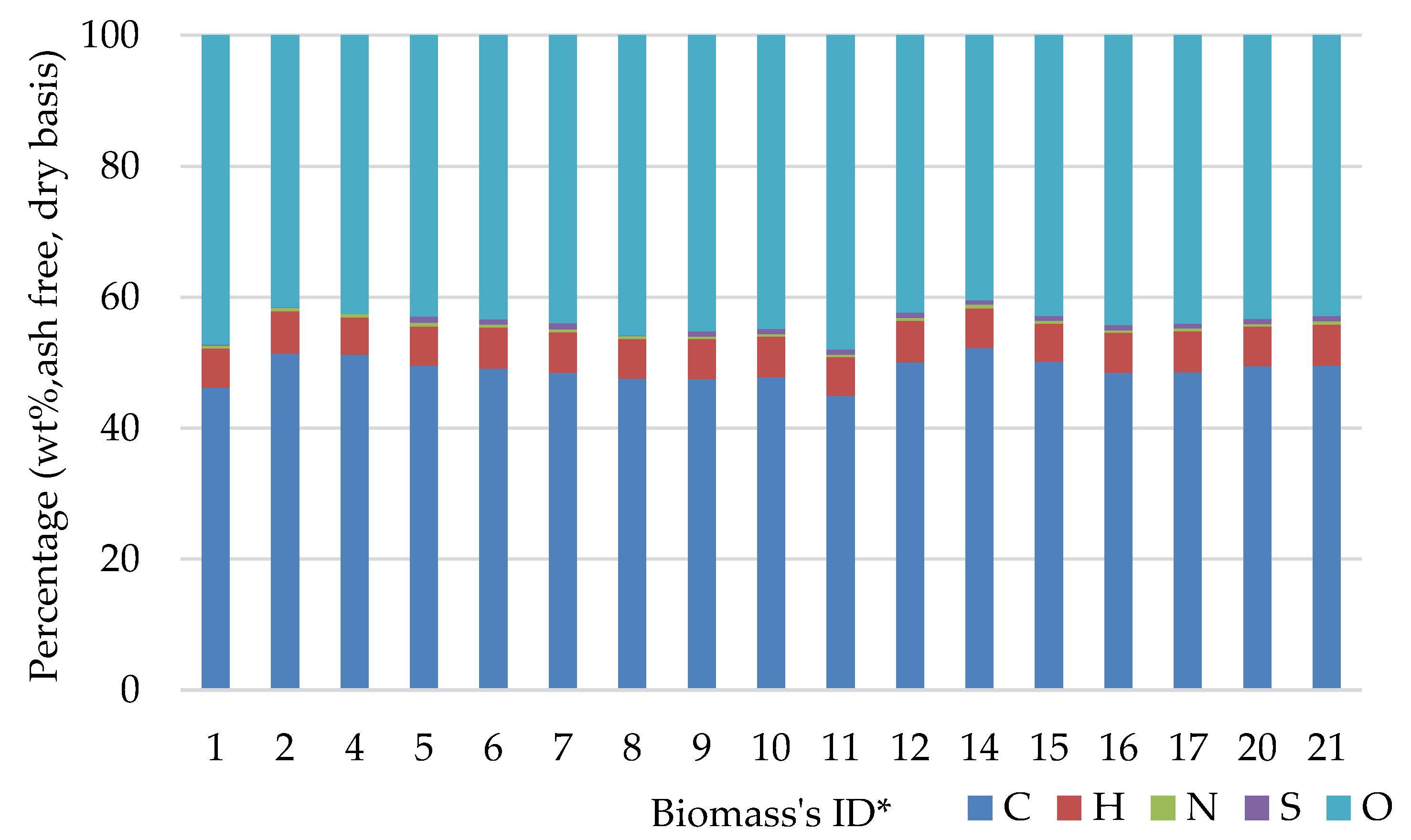
| ID * | Source | Biomass Residues | HHV 1 | C 2 | H 3 | O 4 | N 5 | S 6 |
|---|---|---|---|---|---|---|---|---|
| (MJ/kg) | (wt. %, Ash-Free, Dry Basis) | |||||||
| 1 | [33] | Açaí seed Euterpe oleracea | 18.60 | 47.60 | 6.40 | 45.12 | 0.78 | - |
| 2 | [33] | Banana stem Musa spp. | 16.13 | 39.00 | 5.44 | 54.84 | 0.82 | - |
| 3 | [33] | Banana stalk Musa spp. | 15.73 | 37.95 | 4.73 | 55.85 | 1.46 | - |
| 4 | [33] | Bamboo Guadua sarcocarpa | 18.33 | 43.34 | 5.55 | 48.93 | 0.91 | - |
| 5 | [33] | Coconut Cocos nucifera | 18.70 | 47.40 | 5.41 | 46.64 | 0.55 | - |
| 6 | [32] | Babassu mesocarp Attalea speciosa | 19.07 | 47.13 | 5.17 | 40.70 | 0.27 | - |
| 7 | [30] | Babassu Attalea speciosa | 21.95 | 56.90 | 5.20 | 36.90 | - | - |
| 8 | [29] | Guarana seed Paullinia cupana | 17.58 | 41.55 | 6.44 | 44.91 | 1.51 | - |
| 9 | [31] | Maçaranduba Manilkara huberi | 20.44 | 49.54 | 6.31 | 43.45 | 0.67 | 0.01 |
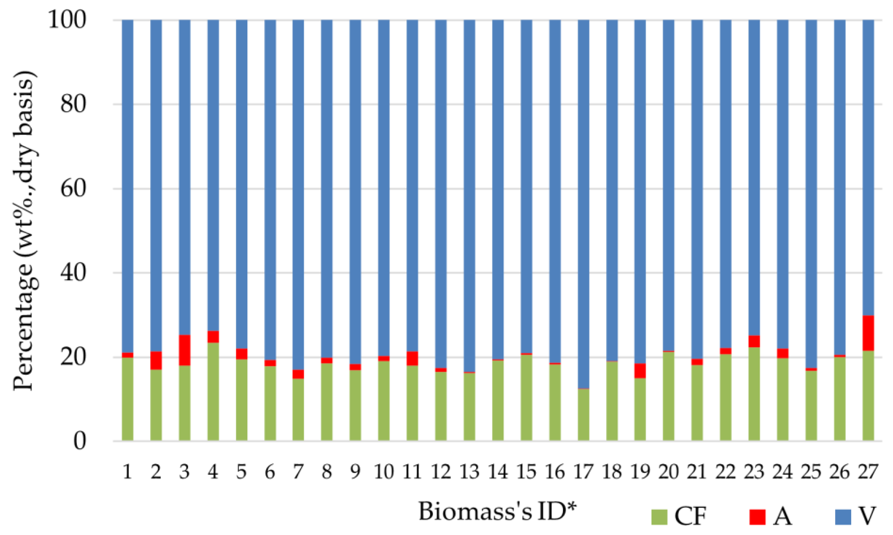
| ID * | Biomass Residues | HHV 1 | V 2 | FC 3 | A 4 | C 5 | H 6 | O 7 | N 8 | S 9 |
|---|---|---|---|---|---|---|---|---|---|---|
| (MJ/kg) | (wt. %, Dry Basis) ª | |||||||||
| 1 | Açaí berry (seed) Euterpe oleracea | 19.23 | 78.88 | 19.91 | 1.21 | 46.16 | 6.01 | 47.26 | 0.43 | 0.13 |
| 2 | Tucumã (seed) Astrocaryum aculeatum | 22.18 | 78.56 | 17.02 | 4.42 | 51.35 | 6.50 | 41.52 | 0.52 | 0.11 |
| 3 | Açaí tree bark (husk) Euterpe oleracea | 16.73 | 74.70 | 17.99 | 7.31 | - | - | - | - | - |
| 4 | Coconut shell (husk) Cocos nucifera | 19.33 | 73.78 | 23.46 | 2.76 | 51.14 | 5.70 | 42.57 | 0.51 | 0.00 |
| 5 | Palm oil kernel shell (PKS) (husk) Elaeis guineensis | 21.22 | 77.92 | 19.55 | 2.53 | 49.55 | 5.96 | 42.92 | 0.60 | 0.96 |
| 6 | Angelim pedra (woody) Hymenolobium modestum | 19.42 | 80.60 | 17.85 | 1.55 | 49.15 | 6.26 | 43.34 | 0.39 | 0.86 |
| 7 | Angelim vermelho (woody) Dinizia excelsa | 20.10 | 82.90 | 14.86 | 2.24 | 48.44 | 6.22 | 43.99 | 0.45 | 0.9 |
| 8 | Bamboo with stripes (woody) Bambusa vulgaris vulgaris | 18.83 | 80.14 | 18.47 | 1.39 | 46.93 | 5.92 | 45.82 | 0.43 | 0.13 |
| 9 | Imperial bamboo (woody) Bambusa vulgaris vittata | 18.76 | 81.64 | 16.97 | 1.39 | 47.48 | 6.14 | 45.21 | 0.35 | 0.82 |
| 10 | Giant bamboo (woody) Dendrocalamus giganteus | 19.56 | 79.73 | 19.09 | 1.18 | 47.82 | 6.15 | 44.83 | 0.37 | 0.83 |
| 11 | Bamboo (woody) Guadua sarcocarpa | 18.80 | 78.63 | 17.96 | 3.41 | 44.96 | 5.90 | 47.99 | 0.39 | 0.77 |
| 12 | Cedro (woody) Cedrela fissilis | 19.83 | 82.60 | 16.54 | 0.86 | 50.10 | 6.34 | 42.37 | 0.37 | 0.82 |
| 13 | Cupiuba (woody) Goupia glabra | 19.37 | 83.44 | 16.20 | 0.36 | 49,09 | 7.83 | 42.52 | 0.19 | - |
| 14 | Ipê amarelo (woody) Handroanthus albus | 21.43 | 80.50 | 19.27 | 0.23 | 52.24 | 6.08 | 40.45 | 0.55 | 0.69 |
| 15 | Jatobá (woody) Hymenaea courbaril | 20.32 | 79.06 | 20.57 | 0.37 | 50.17 | 5.77 | 42.89 | 0.50 | 0.67 |
| 16 | Louro (woody) Ocotea spp. | 20.90 | 81.39 | 18.31 | 0.30 | 48.42 | 6.13 | 44.23 | 0.42 | 0.79 |
| 17 | Marupá (woody) Simarouba amara | 19.66 | 87.42 | 12.38 | 0.20 | 48.53 | 6.28 | 44.05 | 0.41 | 0.73 |
| 18 | Muiracatiara (woody) Astronium ulei | 20.34 | 80.89 | 18.91 | 0.20 | - | - | - | - | - |
| 19 | Pacapeua (woody) Swartzia Racemosa | 18.68 | 81.49 | 15.02 | 3.49 | - | - | - | - | - |
| 20 | Tatajuba (woody) Maclura tinctoria | 19.62 | 78.50 | 21.20 | 0.30 | 49.50 | 6.06 | 43.32 | 0.33 | 0.79 |
| 21 | Timborana (woody) Piptadenia suaveolens | 19.77 | 80.36 | 18.17 | 1.47 | 49.52 | 6.30 | 42.88 | 0.55 | 0.75 |
| 22 | Casca de amêndoa (husk) Prunus dulcis | 22.21 | 77.73 | 20.66 | 1.61 | - | - | - | - | - |
| 23 | Talo de uncária (husk) Uncaria tomentosa | 19.51 | 74.81 | 22.32 | 2.87 | - | - | - | - | - |
| 24 | Tanimbuca (woody) Buchenavia capitata | 19.58 | 78.01 | 19.80 | 2.26 | - | - | - | - | - |
| 25 | Tauari (woody) Couratari tauari | 19.86 | 82.56 | 16.75 | 0.69 | - | - | - | - | - |
| 26 | Pau-preto (woody) Dalbergia melanoxylon | 22.21 | 79.36 | 20.02 | 0.62 | - | - | - | - | - |
| 27 | Uncária (husk) Uncaria tomentosa | 20.77 | 70.10 | 21.49 | 8.41 | - | - | - | - | - |
| Sample mean | 19.74 | 79.66 | 27.60 | 1.79 | 48.19 | 6.25 | 43.79 | 0.43 | 0.77 | |
| Standart deviation | 1.23 | 3.06 | 2.43 | 1.82 | 1.89 | 0.46 | 1.90 | 0.12 | 0.37 | |
| ID * | Biomass Residues | HHV 1 | V 2 | FC 3 | A 4 |
|---|---|---|---|---|---|
| (MJ/kg) | (wt. %, Dry Basis) ª | ||||
| 28 | Angelim (woody) Andira fraxinifolia | 17.50 | 70.01 | 15.13 | 14.86 |
| 29 | Breu (woody) Protium heptaphyllum | 19.90 | 85.62 | 14.19 | 0.19 |
| 30 | Buchas trituradas de dendê (husk) Elaeis guineensis | 17.33 | 72.86 | 15.23 | 9.91 |
| 31 | Cacho seco de amêndoa (husk) Prunus dulcis | 19.34 | 80.55 | 16.60 | 2.85 |
| 32 | Brazil nut shells (husk) Bertholletia excelsa | 20.27 | 71.04 | 27.07 | 1.88 |
| 33 | Walnut shell (husk) Juglans regia L. | 21.08 | 75.86 | 22.49 | 1.65 |
| 34 | Copaíba (woody) Copaifera langsdorffii | 19.90 | 90.87 | 9.05 | 0.08 |
| 35 | Cumaru (woody) Dipteryx odorata | 20.13 | 86.65 | 13.29 | 0.07 |
| 36 | Falso Pau-Brasil (woody) Biancaea sappan | 22.00 | 78.39 | 21.42 | 0.19 |
| 37 | Fibra de coco (husk) Cocos nucifera | 18.65 | 70.60 | 24.67 | 4.73 |
| 38 | Garapa (woody) Apuleia leiocarpa | 18.67 | 78.51 | 18.33 | 3.17 |
| 39 | Louro-Faia (woody) Roupala montana | 19.71 | 82.04 | 17.75 | 0.21 |
| 40 | Maçaranduba (woody) Manilkara bidentata | 20.10 | 82.43 | 17.36 | 0.20 |
| 41 | Mandioqueira (woody) Manihot esculenta | 19.69 | 83.23 | 16.04 | 0.73 |
| 42 | Melancieiro (woody) Alexa grandiflora | 19.96 | 93.87 | 5.36 | 0.77 |
| 43 | Mogno (woody) Swietenia macrophylla | 19.83 | 78.43 | 19.72 | 1.84 |
| 44 | Pau-marfim (woody) Balfourodendron riedelianum | 19.29 | 84.07 | 15.25 | 0.69 |
| 45 | Pequiá (woody) Caryocar brasiliense | 19.87 | 82.63 | 15.60 | 1.77 |
| 46 | Pracuuba (woody) Dimorphandra paraensis Ducke | 20.48 | 80.92 | 18.17 | 0.91 |
| 47 | Quaruba (woody) Vochysia maxima | 18.91 | 81.96 | 17.06 | 0.97 |
| 48 | Coconut shell (husk) Cocus nucifera | 20.54 | 79.74 | 19.30 | 0.95 |
| 49 | Resíduo de Favadanta (husk) Dimorphandra mollis Benth | 19.98 | 76.86 | 19.08 | 4.06 |
| 50 | Roxinho (woody) Peltogyne angustiflora | 19.83 | 80.08 | 19.59 | 0.33 |
| 51 | Sucupira (woody) Pterodon emarginatus | 20.18 | 82.76 | 16.70 | 1.69 |
| 52 | Acapu (woody) Vouacapoua americana | 20.69 | 78.72 | 20.91 | 0.37 |
| 53 | Casca de palmito (husk) Bactris gasipaes | 16.17 | 76.14 | 18.00 | 5.86 |
| 54 | Palm fruit fibre (husk) Elaeis guineensis | 16.54 | 76.21 | 19.59 | 4.20 |
| 55 | Pupunha bark (husk) Bactris gasipaes | 16.64 | 76.24 | 17.63 | 6.13 |
| 56 | Empty palm fruit bunch (EFB) Elaeis guineensis | 18.27 | 84.32 | 15.68 | 2.32 |
| Sample mean | 19.65 | 80.06 | 17.77 | 2.17 | |
| Standard deviation | 1.32 | 5.19 | 3.87 | 3.00 | |
| HHV 1 | V 2 | FC 3 | A 4 | V/FC | FC/V | V/A | FC/A | A/V | A/FC | FC + V | FC + A | V + A | |
|---|---|---|---|---|---|---|---|---|---|---|---|---|---|
| HHV 1 | 1.000 | ||||||||||||
| V 2 | 0.132 | 1.000 | |||||||||||
| FC 3 | 0.218 | −0.795 | 1.000 | ||||||||||
| A 4 | −0.520 | 0.073 | −0.660 | 1.000 | |||||||||
| V/FC | 0.004 | −0.859 | 0.755 | −0.180 | 1.000 | ||||||||
| FC/V | 0.063 | 0.985 | −0.870 | 0.215 | −0.823 | 1.000 | |||||||
| V/A | 0.072 | −0.342 | 0.374 | −0.196 | 0.308 | −0.342 | 1.000 | ||||||
| FC/A | 0.128 | −0.283 | 0.365 | −0.256 | 0.256 | −0.297 | 0.974 | 1.000 | |||||
| A/V | −0.507 | 0.079 | −0.664 | 0.999 | −0.182 | 0.222 | −0.186 | −0.243 | 1.000 | ||||
| A/FC | −0.520 | −0.050 | −0.560 | 0.983 | −0.071 | 0.089 | −0.180 | −0.238 | 0.982 | 1.000 | |||
| FC + V | 0.523 | −0.064 | 0.656 | −0.995 | 0.174 | −0.206 | 0.190 | 0.248 | −0.994 | −0.983 | 1.000 | ||
| FC + A | −0.206 | 0.808 | −0.998 | 0.647 | −0.763 | 0.880 | −0.377 | −0.367 | 0.650 | 0.543 | −0.637 | 1.000 | |
| V + A | −0.113 | −0.996 | 0.814 | −0.102 | 0.861 | −0.986 | 0.344 | 0.285 | −0.108 | 0.019 | 0.100 | −0.822 | 1.000 |
| ID * | Equation | F. | p-Value | MAPE | |
|---|---|---|---|---|---|
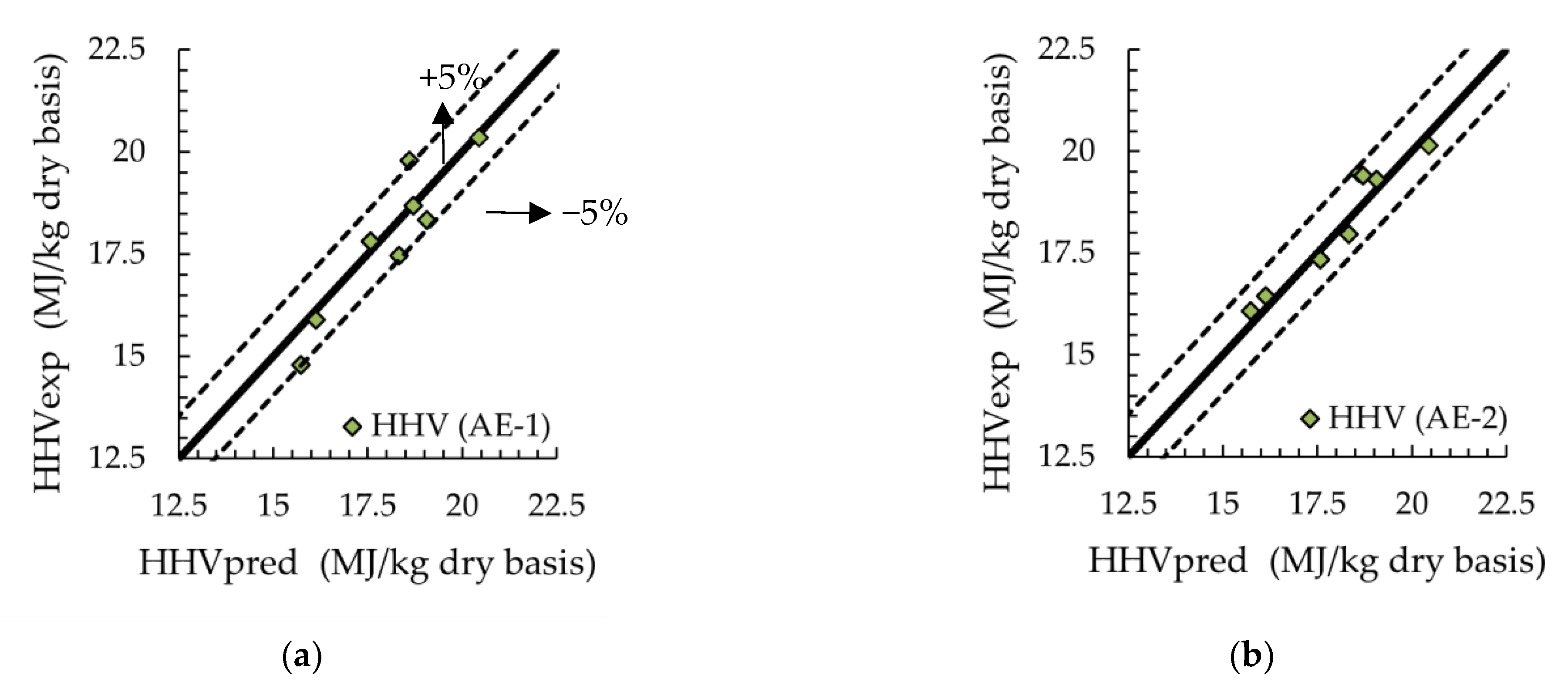
| AI-1 | HHV = 0.196 × V + 0.221 × FC | 0.94 | 0.00 | 0.02 | 4.19% |
| AI-2 | HHV = 0.204 × (V + FC) − 0.128 A | 0.95 | 0.00 | 0.31 | 4.35% |
| HHV | C | H | N | S | O | |
|---|---|---|---|---|---|---|
| HHV | 1.000 | |||||
| C | 0.899 | 1.000 | ||||
| H | 0.502 | 0.447 | 1.000 | |||
| N | −0.612 | −0.736 | −0.122 | 1.000 | ||
| S | 0.499 | 0.481 | 0.345 | −0.544 | 1.000 | |
| O | −0.808 | −0.848 | −0.573 | 0.477 | −0.366 | 1.000 |
| ID * | Equation a | F. | p-Value | MAPE | |
|---|---|---|---|---|---|
| AE-1 | HHV = 2.957 + 0.335 × C + 1.064 × H | 0.49 | 0.01 | 0.26 | 2.98% |
| AE-2 | HHV = 2.765 + 0.351 × C | 0.57 | 0.00 | 0.00 | 2.84% |
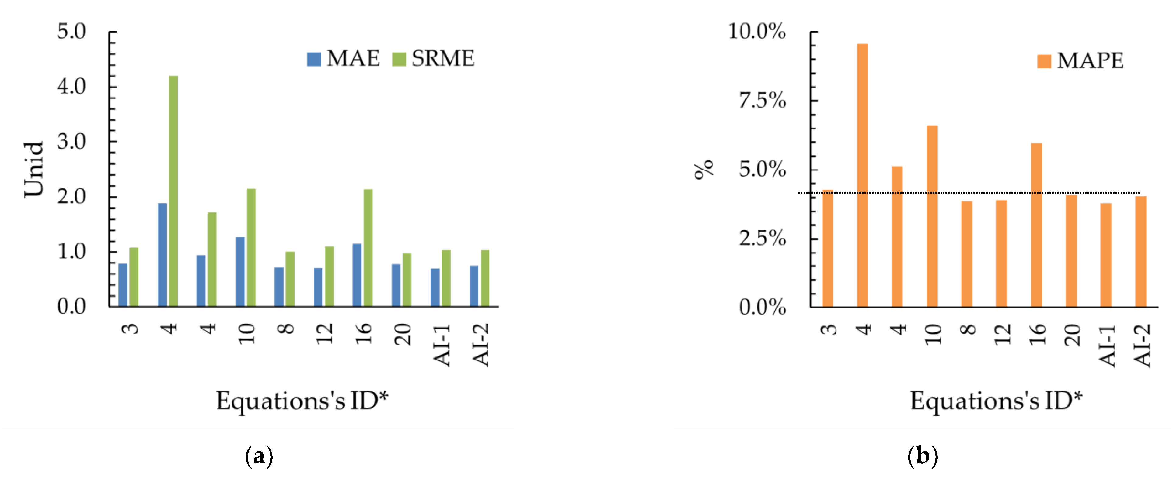
| ID | This Work 1 | MAE | MAPE | SRME |
|---|---|---|---|---|
| AI-1 | HHV = 0.196 × V + 0.221 × FC | 0.70 | 3.79% | 1.04 |
| AI-2 | HHV = 0.204 × (V + FC) − 0.128 A | 0.75 | 4.04% | 1.04 |
| ID | This Work 1 | MAE | MAPE | SRME |
|---|---|---|---|---|
| AE-1 | HHV = 2.957 + 0.335 × C + 1.064 × H | 0.42 | 2.85% | 0.64 |
| AE-2 | HHV = 2.765 + 0.351 × C | 0.20 | 2.20% | 0.45 |
Publisher’s Note: MDPI stays neutral with regard to jurisdictional claims in published maps and institutional affiliations. |
© 2022 by the authors. Licensee MDPI, Basel, Switzerland. This article is an open access article distributed under the terms and conditions of the Creative Commons Attribution (CC BY) license (https://creativecommons.org/licenses/by/4.0/).
Share and Cite
Moreira, J.; Carneiro, A.; Oliveira, D.; Santos, F.; Guerra, D.; Nogueira, M.; Rocha, H.; Charvet, F.; Tarelho, L. Thermochemical Properties for Valorization of Amazonian Biomass as Fuel. Energies 2022, 15, 7343. https://doi.org/10.3390/en15197343
Moreira J, Carneiro A, Oliveira D, Santos F, Guerra D, Nogueira M, Rocha H, Charvet F, Tarelho L. Thermochemical Properties for Valorization of Amazonian Biomass as Fuel. Energies. 2022; 15(19):7343. https://doi.org/10.3390/en15197343
Chicago/Turabian StyleMoreira, João, Alan Carneiro, Diego Oliveira, Fernando Santos, Danielle Guerra, Manoel Nogueira, Hendrick Rocha, Félix Charvet, and Luís Tarelho. 2022. "Thermochemical Properties for Valorization of Amazonian Biomass as Fuel" Energies 15, no. 19: 7343. https://doi.org/10.3390/en15197343