Energy Saving Evaluation with Low Liquid to Gas Ratio Operation in HVAC&R System

Abstract

Previous studies have been conducted by employing various methods to reduce the condenser water temperature, a crucial control variable to consider when attempting to improve the operational efficiency of a chiller. The existing literature dealing with the effects of low-condenser water temperatures is limited, as the cooling water flow rate is often considered the operating variable of the condenser loop. However, to produce additional low condenser water temperatures, the approach temperature of the cooling tower in the system must be reduced. To reduce the approach temperature, it is necessary to review the physical behavior and efficiency of the cooling tower according to the change in the liquid to gas ratio (LGR), which is dependent upon the condenser water flow rate and the cooling tower fan air flow rate within the condenser loop. However, this process has rarely been reviewed in previous studies. Therefore, this study developed a new cooling tower control algorithm from the LGR perspective, and the operational effectiveness was quantitatively reviewed using EnergyPlus. Compared to the conventional conditions, when the cooling tower operation algorithm for low-approach temperatures was applied, the annual energy saving was 27.0%, the average chiller COP was improved by 27.8%, and the average system COP was improved by 47.4%. Furthermore, even when the algorithm was not applied at the same condenser water set temperature, the annual energy saving was 15%. The average COP of the chiller and COP of the system is improved by 2% and 23.2%, respectively. These results indicated that when a cooling tower is operated with a low LGR, even under the same outdoor air and load conditions, the cooling system’s efficiency can be improved with a change in the control algorithm without installing additional high-efficiency equipment.

1. Introduction

1.1. Background

Cooling energy accounts for around 20% of the total energy consumption of a typical building [1]. With an average temperature increase of 1 °C, a 25% increase in cooling degree days is predicted. The demand for cooling energy is expected to triple by 2050 due to the larger global population and higher income. Thus, improving the efficiency of cooling systems in buildings is essential for energy savings.

A water-cooled central chilled water system is commonly used in large commercial buildings. The energy consumption of the chiller is approximately three to four times larger than the sum of the other components, such as cooling tower fans and pumps. Thus, improving the efficiency of chillers can significantly impact the cooling energy savings [2,3]. Various parameters should be considered to increase the coefficient of performance (COP), representing the chiller’s efficiency [4,5,6,7,8,9]. The parameters include the chiller’s outlet temperature, the condenser inlet temperature (from now on referred to as a condenser water temperature), the part-load ratio, the sequencing control, the system configuration, and the weather conditions. Among them, the smaller the condenser water temperature change according to the outdoor wet-bulb temperature, and the lower the condenser water temperature, the greater the efficiency of a vapor-compression-based cooling system. When the condenser water temperature was decreased by 1 °C, the total cooling energy consumption was reduced by 3% to 5% [10]. However, despite the effects of this efficiency improvement, general cooling tower designs and controls are operated with a fixed condenser water temperature according to the rated conditions, so maximized efficiency operation is not possible [3,11]. Therefore, to improve the efficiency of the water-cooled central chilled water system, it is necessary to review a cooling tower control-based method for lowering the condenser water temperature.

1.2. Literature Review

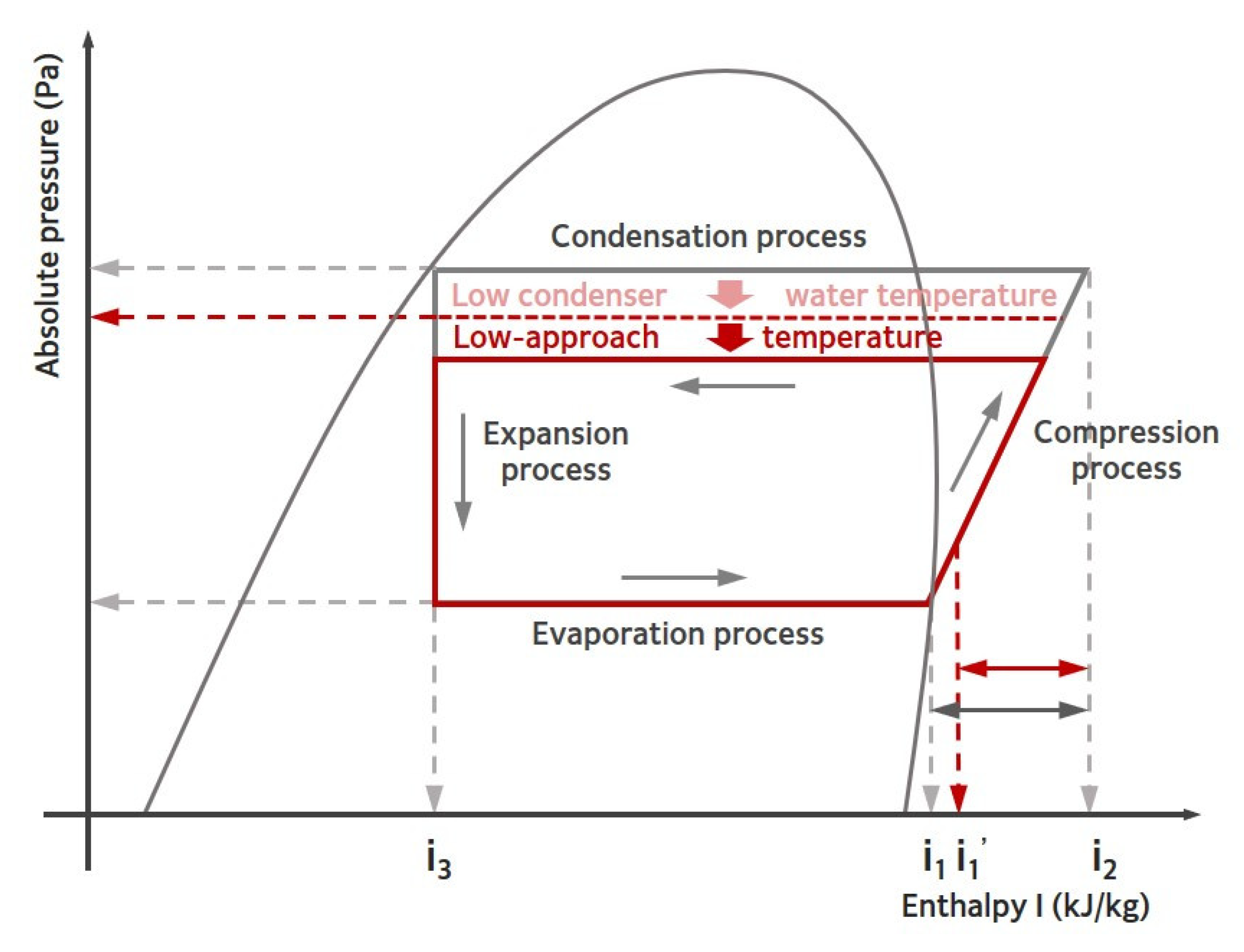
1.2.1. Influence of Low-Condenser Water Temperature on Cooling System

Studies have been conducted on various control methods for producing low-temperature condenser water [3,12,13,14,15,16,17,18,19]. Liu and Chuah [14] applied an optimal approach temperature control strategy per hour to reset the condenser water temperatures for commercial buildings in Taiwan, aiming to improve the performance of chillers and cooling tower systems. Their results verified a greater than 4% energy-saving effect annually compared to existing control methods. Yao et al. [15] optimized a model-based cooling system to obtain an optimal condenser water temperature and flow rate, thereby reducing the system’s cooling energy consumption by around 10%. Zhang et al. [16] minimized the cooling plant system’s energy consumption by utilizing an optimal cooling tower outlet temperature, chiller load, and condenser water flow rate. Huang et al. [3] applied a predictive control model to improve the efficiency of legacy chiller plants. Their method determined the optimal condenser water set temperature based on the relationship between the cooling load and the outdoor air wet-bulb temperature without altering the control scheme. The required annual cooling energy of the chiller and the cooling tower was reduced by up to 9.57%. They also used a Bayesian network model and reduced energy usage by 25.92% in the cooling season and by 1.39% in the intermediate seasons due to the use of the optimal condenser water set temperature, which was lower than the existing fixed condenser water set temperature (26.1 °C) [17]. Kang et al. [18] developed an artificial neural network-based real-time prediction control and optimization algorithm to save on cooling energy in the chiller-based cooling system of a specific building. The outlet temperature range (25–32 °C) of the cooling tower and the chilled water inlet temperature range (6–12 °C) of the chiller was selected, and the average energy savings rate was 7.4%, while the COP improved by 9.4% on average. Lee et al. [19] verified the low-temperature condenser water effect by controlling the condenser water flow rate of a large-sized office building system. Although the condenser water temperature during general operations was primarily distributed around 32 °C, a lower condenser water temperature, 24 °C, could be produced when the flow control algorithm was applied. As a result, a 24% energy saving and a 5.9% reduction in an outdoor unit’s variable refrigerant flow (VRF) due to the low-temperature condenser water were achieved. The COP of the outdoor unit and the system improved by 7.3% and 12.7%, respectively. Tae Young Kim et al. [20] showed that, through ANN-based real-time condenser water optimal control, energy was saved by about 5.6% compared to the conventional cooling water temperature control fixed at 30 °C. However, the author does not mention the cooling water temperature control by changing the approach temperature.

The studies above produced low condenser water temperatures using various control methods, verifying cooling energy savings and improved system efficiency compared to existing control methods. Existing studies [4,5,18,19,21] set the condenser water temperature according to the climate zone of the pertinent region, and the condenser water flow rate acted as the primary control variable to produce low condenser water temperatures [5,18,19].

However, the set temperature of the condenser water was set at the lower limit temperature of the chiller specifications. In addition, the process of producing a low-condenser water temperature in a cooling tower was determined by the condenser water flow rate and the cooling tower fan air flow rate (from now on, referred to as LGR). Without considering the control sequence and the influence of these two control variables, no matter how advanced the methodology, there is a limit to lowering the condenser water temperature. Therefore, to produce a lower condenser water temperature than in the existing studies, it is necessary to review the operating effect from the LGR viewpoint.

1.2.2. Liquid to Gas Ratio

Generally, LGR values are reviewed from the design viewpoint of the cooling tower. However, LGR values are also examined from the operation control viewpoint [22,23,24], as a reduction in LGR values indicates an increase in the airflow rate compared to the condenser water flow rate inside the cooling tower, an increase in the contact area between the condenser water and the fill material, and an increase in the residence time of the fill material in the condenser water. This leads to an improvement of the heat transfer capacity, thereby increasing the number of transfer units that share the characteristic values of the fill material, thereby improving the heat rejection rate in the cooling tower [25,26,27]. As the LGR value decreases, the efficiency of the cooling tower is improved, and the approach temperature can be reduced. The reduction of the approach temperature leads to a lower condenser water temperature, and thus the temperature range of the cooling tower is increased. The conveying energy is reduced, and the COP of the chiller is improved due to the decrease in the flow rate of the condenser water [28]. Therefore, there is a need for a cooling tower-based control method to lower LGR values. It is necessary to reduce the approach temperature and quantitatively review the energy performance from the system’s perspective.

As mentioned above, the efficiency of the cooling tower changes according to the LGR value, which indicates a degree of success in utilizing the cooling potential of the ambient air for cooling towers. There are studies on the efficiency of cooling towers according to changes in LGR values from the operational viewpoint [29,30,31,32]. Siphon [29] studied the heat transfer and pressure drop characteristics according to the LGR through experimental and mathematical methods. Costelloe and Finn [30] reviewed the number of transfer units (NTU) required for a low approach temperature (1–3 K) of an open cooling tower in a temperate maritime climate in a building where a chilled ceiling was installed. Their study results showed that as the heat performance of the cooling tower changed according to the change in the LGR, the NTU level increased when the LGR was 0.3–0.9. Nasrabadi and Finn [31] developed a mathematical model to minimize the approach temperature of an open cooling tower in a building where a radiant cooling system was applied through experiments. They analyzed the configurations of the cooling towers, which changed according to the ambient boundary conditions and the condenser water temperature. They reviewed the effects of the cooling tower’s coefficient on the cooling tower’s outlet temperature and heat rejection. In addition, [32] they examined the performance under four different climate conditions and the main parameters of the cooling tower based on verified mathematical models. It was determined that a low approach temperature concerning the ambient air wet-bulb temperature could be achieved down to 2 K under all climate conditions. A 1 K approach temperature was feasible only in warm and humid climates.

The above studies [29,30,31,32] identified the efficiency of cooling towers and changes in the approach temperatures according to LGR values and climate conditions with only a cooling tower system (condenser loop). However, no studies have been conducted to review a cooling system’s efficiency and energy savings, including the chiller. In addition, most studies have not dealt with the physical behavior of cooling towers, efficiency improvements, and lowered approach temperature according to changes in LGR values under dynamic building operating conditions, such as the installation of outdoor air conditions, internal heat gain, and changing cooling loads.

In this study, a new cooling tower control algorithm was developed from the LGR perspective to increase the overall system efficiency of water-cooled central chilled water systems. A water-cooled chilled water system, from the cooling tower to the chilled water header, was modeled using EnergyPlus. The developed control algorithm was applied through an EnergyPlus-Python co-simulation. The study selected three viewpoints: intermediate seasons, cooling season, and an annual period for the simulation to analyze the operational efficiency quantitatively and comparatively (energy cut-off, improvement of system efficiency, low-condenser water temperature production, and the reduction effects of approach temperature) of the developed LGR algorithm compared to that of existing cooling tower control methods having the same system specifications.

1.3. Contributions

The contribution of this study is to develop a new control algorithm for the low condenser water temperature of cooling towers from the perspective of the LGR, considering changing outdoor air conditions and the cooling loads of the buildings in real-time, specifically as follows:

• Considering the chiller equipment specifications, a perspective on the condenser water set temperature is presented to produce a lower low-approach temperature than the low-condenser water temperature according to existing climatic conditions.
• It is essential to understand the relationship between five variables (ambient wet-bulb temperature, heat rejection load of cooling tower, approach temperature [33], condenser water flow rate, and cooling tower fan air flow rate) to produce low-condenser water temperatures that change in real-time without relying on rules of thumb. A control sequence was developed, taking these variables into account.
• Using the LGR value from an operation control point of view, the physical behavior of the cooling tower, efficiency improvements, and decreased approach temperatures were identified. In addition, the effect on the overall efficiency improvements of the chiller and central chilled water system were evaluated quantitatively.
• Efficiency improvements in the central chilled water system currently operating in buildings without adding efficiency devices can be expected only when changing the cooling tower control algorithm.

The remainder of this study is organized as follows: Section 2 briefly describes the efficiency improvement methods reviewed and explains the newly developed cooling tower control algorithm. Section 3 describes the target building and physics-based HVAC&R system modeling. Section 4 compares and analyzes the calculation results for each simulation case. Section 5 provides a conclusion.

2. Methodology

The temperature range ($T_{Range})$ of the cooling tower is defined as the difference between the inlet and outlet temperature of the cooling tower ($T_{out,cw}-T_{in,cw}$). The approach temperature ($T_{approach}$) of the cooling tower is defined as the difference between the outlet temperature of the cooling tower and the outdoor air wet-bulb temperature ($T_{in,cw}$ − $T_{in, wb}$). Figure 1 was constructed concerning Ref. [34]. The study depicted focused on increasing the evaporation temperature of the chiller. However, this study focuses on decreasing the condenser water temperature. The liquid to gas ratio (hereinafter referred to as LGR) is defined as the ratio of condenser water flow rate to cooling tower fan airflow rate. In Figure 1, as the length of the arrow decreases, the height of the cooling cycle decreases due to the reduction of refrigerant pressure of the chiller, as shown in Figure 2. Accordingly, the compressor’s power consumption is reduced, and the chillers’ COP is increased. Therefore, in this study, the operation efficiency is reviewed by securing the lowest condenser water temperature within the operating range of the cooling tower. In this paper, a condenser water temperature lower than the rated condition of the existing cooling tower is defined as a low-condenser water temperature, and a lower temperature than that of the low-condenser water temperature is defined as a low-approach temperature.

2.1. Study Scope

This study developed a new cooling tower operation control algorithm from the LGR perspective by changing the cooling water set temperature according to the chiller specifications. This study quantitatively and comparatively analyzed energy performance through dynamic simulations to review the operational efficiency of the developed algorithm and condenser water temperatures. Accordingly, this study employed EnergyPlus v.9.5, a building energy simulation program that can model a building and heating, ventilation, air conditioning, and refrigeration (HVAC&R) system and conduct sensitivity analysis. The results were compared to the general cooling tower control methods specified in Korean Standards (KS). The control measure was divided into three, considering the condenser water set temperature and LGR values, which are variables that can be considered during cooling tower operations. The three control measures proposed in this study were: (1) change the condenser water set temperature (Section 2.2.1), (2) review the low approach temperature according to changes in the LGR (Section 2.2.2), and (3) application of the integrated cooling tower to the cooling tower system (Section 2.2.3). Finally, this study aimed to review the system energy consumption and efficiency according to the classified cases and identify the operational efficiency of low LGR in the cooling tower by identifying the production time of the condenser water temperature. Figure 3 shows the overall flow chart of this study.

2.2. Cooling Tower’s Efficiency Improvement Strategy

Figure 4 depicts the strategy to improve the efficiency of cooling tower operations. Cases are categorized as conventional LGR, high LGR (if the LGR value was 1.2 higher than the designed conditions), and low LGR (if the LGR value was 1.2 lower than the designed conditions).

2.2.1. Condenser Water Set Temperature Change

The consumption of power by the compressor was reduced due to the refrigerant pressure drop as low-condenser water was produced, thereby improving the COP, which is the performance coefficient of the chiller. Accordingly, the condenser water set temperature, the primary variable to improve performance and save energy in the chiller, was changed by case.

It is common to perform on/off controls of the cooling tower fan while fixing the condenser water flow rate, thus leaving the temperature as the rated temperature when the water-cooled chiller uses the cooling tower method, as many offices do in Korea [35]. In Case A, 32 °C is the rated condition of the cooling tower according to KS specifications. In Case B, 23.9 °C, corresponding to Seoul’s temperature (Climate zone 4A), proposed in ASHRAE 90.1, was used [36]. This temperature was chosen arbitrarily because the lower condenser water temperature limits differ depending on the chiller manufacturer, although every manufacturer sets a value to maintain stability during the cooling cycle. In Cases C–E, 14 °C, which included a safety factor of about 10% to 12.78 °C, the lower limit temperature of the chiller model (Carrier 19XR) specifications was applied [37]. This allowed the cooling tower to run conservatively, ensuring the stability and robustness of the system.

2.2.2. Review of the Low Approach Temperature According to Changes in the LGR

Section 2.2.1 focused on the change in the condenser water set temperatures. However, this change can cause a problem—low delta-T syndrome in the condenser water loop side of a hydronic system as the cooling tower control method continues to be operated using conventional LGR standards. Low delta-T syndrome is one of the main operational problems that degrade the energy performance of a cooling system [38,39]. If the flow rate and pressure are not controlled correctly in a hydronic system on the condenser water loop side, the efficiency of the cooling tower degrades due to the excessive flow of low condenser water, which increases the conveyance energy of the condenser water pump, and induces a higher LRG value. As a result, it can produce a high approach temperature regardless of the cooling tower specifications. In particular, a high approach temperature may lead to a high condenser water temperature entering the chiller’s condenser, thereby degrading the efficiency of the entire cooling system and increasing energy consumption.

To overcome this, Case D employs a lower LGR, rather than a conventional LGR, through a change in the control algorithm of the cooling tower. Generally, LGR is considered during the design of a cooling tower. However, it can be utilized from the operation control viewpoint to improve efficiency, as it can improve the cooling tower due to the change in heat transfer performance. Accordingly, the condenser water flow rate should be reduced, and the fan air flow rate in the cooling tower should be increased to obtain a lower LGR.

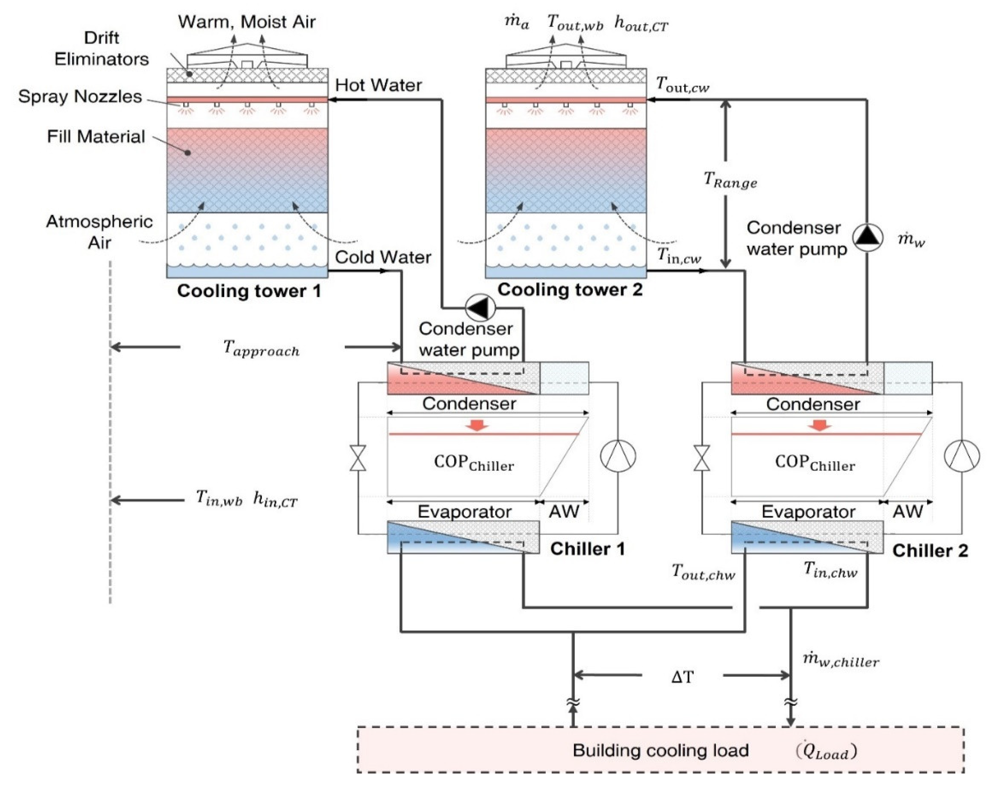
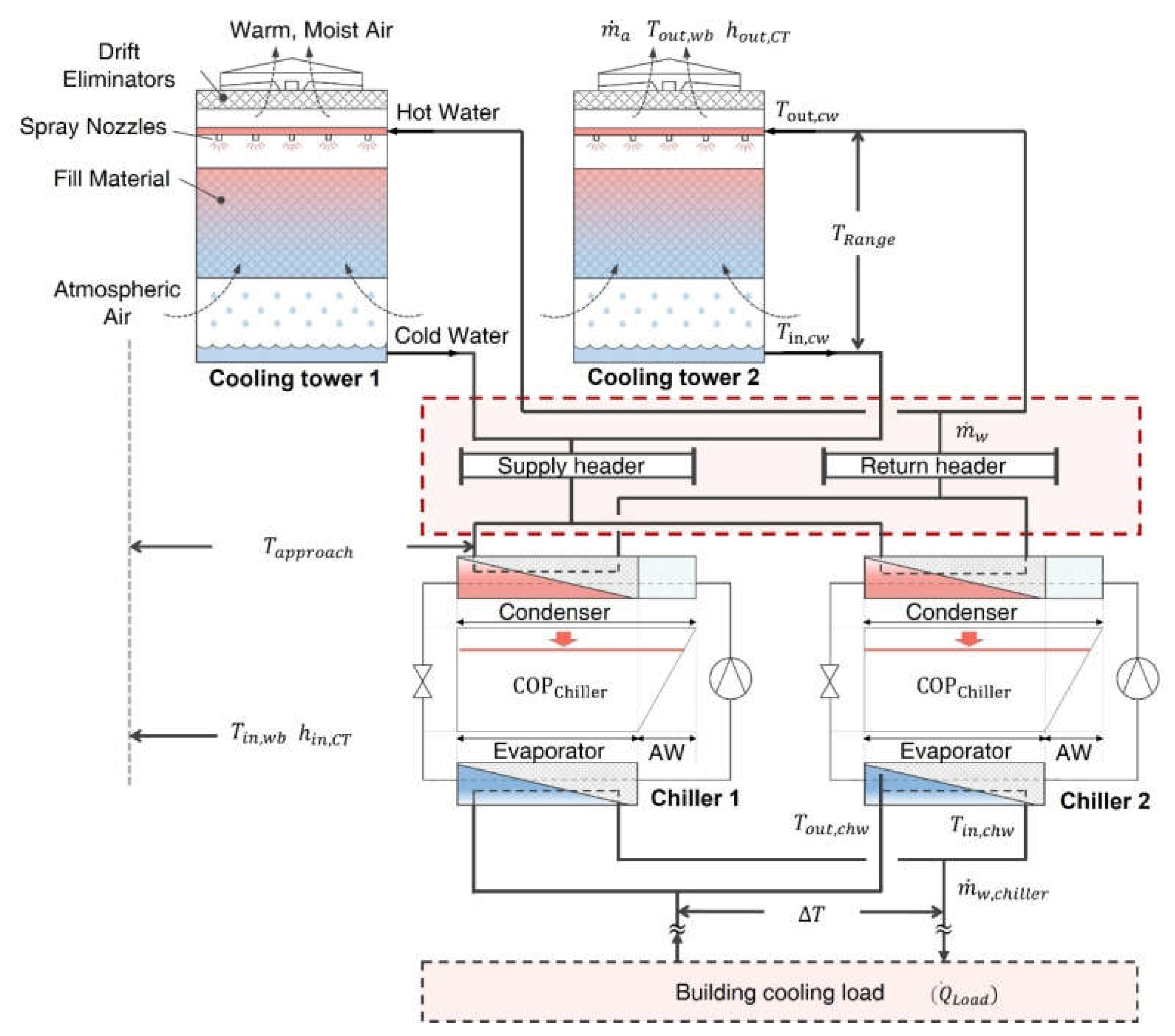
2.2.3. Integrated Cooling Tower

As shown in Figure 5, the ratio of the cooling tower to a chiller in Cases A–D is generally 1:1. In other words, one chiller is connected to one cooling tower. However, the cooling capacity increases as the airflow rate increases in a cooling tower compared to the constant flow rate of condenser water. Thus, an approach temperature of 1–2 K can be achieved. Still, the cooling capacity has to be increased up to six times the rated value depending on climate, which is a drawback. This may lead to an unrealistically excessive design of a cooling tower. Therefore, a measure was proposed to reduce the condenser water flow rate [32]. However, if the condenser water flow rate is decreased excessively, overheating in the pump and a temperature rise in the chiller condenser may occur. Thus, previous studies [29,30,31,32] only considered the performance of a single cooling tower, which is a limitation. To overcome this limitation and review higher LGR operation efficiency compared to Case D, Case E integrated existing cooling tower hydronics, as shown in Figure 6, to model an integrated cooling tower, which has a high operating cost [40], aiming to increase the airflow rate in the cooling tower without increasing the rated capacity.

2.3. Development of Cooling Tower Control Algorithm

Co-Simulation

To maintain control with the low LGR of Cases D and E, the cooling system should be equipped with a variable-speed cooling tower and a variable-speed condenser water pump for the control of air flow rate in the cooling tower fan and the flow rate of the condenser water pump inside the condenser water loop system, respectively. However, in the current EnergyPlus simulation program, the flow rate of the condenser water pump is constantly maintained at the maximum flow rate whenever the chiller is operated, regardless of the cooling load of the building, and the variable-speed condenser water pump and the variable speed control of the cooling tower fan cannot be modeled, which is a drawback [41,42]. As mentioned in Section 2.2.2, if the flow rate of the condenser water pump is maintained at the maximum and the air flow in the cooling tower fan is reduced, there is a conventional LGR result. The conventional LGR leads to low delta-T syndrome inside the condenser loop, and a low approach temperature cannot be obtained. Thus, this study integrated EnergyPlus and Python v.3.9.5, an open-source programming language, to solve the variable condenser water pump modeling issue. An embedded Python interpreter was added to EnergyPlus v. 9.3, and Energy Management System (EMS) end points (e.g., sensor, actuator, and meter) were wrapped into the Python programming interface (API), allowing users to write EMS programs. Python is equipped with various libraries for functions varying from scientific calculations to machine learning. It can also interact with web APIs and detect and control hardware. In addition, EMS scripts written by users can be made as portable packages that can be modified and used by others using Python [43,44]. Users can program the EMS objects in EnergyPlus by selecting algorithms using Python programming scripts and control them in real-time.

Table 1. Data exchange between EnergyPlus and Python.

EnergyPlus to Python	Python to EnergyPlus
Cooling tower heat transfer rate [kW]	Cooling tower air flow rate [kg/s]
Outdoor dry-bulb temperature [°C]	condenser water flow rate [kg/s]
Outdoor relative humidity [%]	Outdoor wet-bulb temperature [°C]
Design cooling tower heat transfer rate [kW]	Cooling tower inlet temperature [°C]
Design cooling tower water flow rate [kg/s]	Cooling tower outlet temperature [°C]

presents the data items exchanged in real-time between EnergyPlus and Python.

2.4. Cooling Tower Control Algorithm for Low Approach Temperature

In this section, the control algorithm implemented through co-simulation is explained. The performance of the cooling tower can be exhibited through approach temperatures and changes according to the cooling tower inlet and outlet temperature, the ambient air’s wet-bulb temperature, the condenser water flow rate, and the air flow rate of the cooling tower fan. A cooling system designer provides the first four variables, but the cooling tower manufacturer determines the air flow rate [28]. Thus, for an operator to lower the approach temperature without depending on rules of thumb, it is important to consider the relationship among all variables.

Accordingly, this study developed a cooling tower control algorithm that can calculate a low approach temperature considering the five variables that dynamically change within the system, as shown in Figure 7. The algorithm is reflected in Cases D–E. Outdoor air wet-bulb temperature, LGR, and the temperature range are independent variables and are calculated to obtain the approach temperature, a dependent variable in Equation (5). In addition, because the approach temperature is a value that changes according to the LGR under the same outdoor air and load conditions, the algorithm was made by focusing on maintaining a low LGR in every control step. The approach temperature can be lowered through the improvement of efficiency in heat transfer of the cooling tower as the LGR value is lowered, which leads to the production of low-temperature condenser water, leading to the expected improvement of the chiller COP and a reduction in the condenser water flow rate.

The initial input data required for the control algorithm are the outdoor air dry-bulb temperature and relative humidity, the condenser water set temperature, the condenser water pump flow rate, the cooling tower air flow rate, the cooling tower heat rejection rate, and the on/off of the condenser water pump operations. Using this input data, the control variables required for the reduction of approach temperature were calculated.

Generally, an outdoor air wet-bulb temperature can be measured using a wet-bulb thermometer, but this data is difficult to acquire inside most buildings. Thus, an outdoor air dry-bulb temperature and the relative humidity measured in the building were requirements for Equation (1) [45] to calculate the approximate outdoor air wet-bulb temperature. As the condenser water is affected by the outdoor air wet-bulb temperature, it is important to address this issue.

$$\begin{array}{cc}{T}_{in,wb}=T_{db}·\hfill & atan\left[0.151977{\left(\omega +8.313659\right)}^{0.5}\right]+atan\left(T_{db}+\omega \right)\hfill \\ & -atan\left(\omega -1.676331\right)+0.00391838{\left(\omega \right)}^{1.5}\hfill \\ & ·atan\left(0.023101\omega \right)-4.686035\hfill \end{array}$$

(1)

where, $T_{db}$ refers to the outdoor dry-bulb temperature (°C), $\omega$ refers to the outdoor relative humidity (%), and $T_{in,wb}$ refers to the outdoor wet-bulb temperature (°C).

The operation status of the cooling system can be determined by the on or off status of the condenser water pump and the condenser water flow rate, which were calculated through Equation (2). To solve the problem that a variable condenser water pump controlled though the aforementioned variables cannot reflect changes in the building cooling load, this study controlled the condenser water flow rate in real-time according to the cooling tower heat rejection rate.

$${\dot{m}}_w={\dot{m}}_{Ref,w}·\frac{{\dot{Q}}_{HR,CT}}{{\dot{Q}}_{Ref,CT}}$$

(2)

where, ${\dot{m}}_w$ refers to the condenser water flow rate (kg/s),${\dot{m}}_{Ref,w}$ refers to the condenser water flow rate (kg/s) at the rated condition, ${\dot{Q}}_{HR,CT}$ refers to the cooling tower heat rejection rate (kcal/h), and ${\dot{Q}}_{Ref,CT}$ refers to the cooling tower heat rejection rate (kcal/h) at the rated condition.

According to the EnergyPlus Engineering Ref. [46], the variable-speed cooling towers empirical model applied in this study to produce a low approach temperature determines the cooling tower outlet temperature by running the cooling tower fan at the peak rate. When the cooling tower outlet temperature is higher than the condenser water set temperature, the cooling tower fan continues to run at the peak rate. The LGR, which is a ratio of the condenser water pump flow rate to the cooling tower fan air flow rate, was calculated using Equation (3), where ${\dot{m}}_a$ refers to the cooling tower air flow rate (kg/s).

$$\mathrm{LGR}=\frac{{\dot{m}}_w}{{\dot{m}}_a}$$

(3)

The temperature range ($T_{Range})$, which is the temperature difference between the condenser water entering and leaving the tower ($T_{out,cw}$ − $T_{in,cw}$), was calculated via Equation (4), where $C_{pw}$ is 4.185 kJ/kg, the specific heat value of water. As the temperature range becomes larger as the condenser water flow rate, calculated in Equation (2), decreases, it can be interpreted as a changing value according to the cooling load.

$$T_{Range}=\frac{{\dot{Q}}_{HR,CT}}{{\dot{m}}_w·C_{pw}}$$

(4)

The approach temperature ($T_{approach})$, which is the difference between the cooling tower outlet temperature and inlet air wet-bulb temperature and represents the performance of the cooling tower. The heat rejection temperature is determined by the cooling capacity of the cooling tower and the outdoor air wet-bulb temperature [47]. The approach temperature in the YorkCalc model of the variable-speed cooling tower, applied in this study, can be calculated through Equation (5). Where, ${\beta }_1$–${\beta }_{27}$ refer to the coefficients that represent the characteristics of the YorkCalc cooling tower models proposed in the Engineering Ref. [46], which are presented in

Table 2. Cooling tower model coefficients.

${\mathit{\beta }}_1$	${\mathit{\beta }}_2$	${\mathit{\beta }}_3$	${\mathit{\beta }}_4$	${\mathit{\beta }}_5$
−0.359741205	−0.055053608	0.0023850432	0.173926877	−0.0248473764
${\beta }_6$	${\beta }_7$	${\beta }_8$	${\beta }_9$	${\beta }_{10}$
0.00048430224	−0.005589849456	0.0005770079712	−1.342427256 × 10−5	2.84765801111111
${\beta }_{11}$	${\beta }_{12}$	${\beta }_{13}$	${\beta }_{14}$	${\beta }_{15}$
−0.121765149	0.0014599242	1.680428651	−0.0166920786	−0.0007190532
${\beta }_{16}$	${\beta }_{17}$	${\beta }_{18}$	${\beta }_{19}$	${\beta }_{20}$
−0.025485194448	4.87491696 × 10−5	2.719234152 × 10−5	−0.06537662555556	−0.002278167
${\beta }_{21}$	${\beta }_{22}$	${\beta }_{23}$	${\beta }_{24}$	${\beta }_{25}$
0.0002500254	−0.0910565458	0.00318176316	3.8621772 × 10−5	−0.0034285382352
${\beta }_{26}$	${\beta }_{27}$
8.56589904 × 10−6	−1.516821552 × 10−6

. They differ according to the model and performance of the cooling tower. The approach temperature, a dependent variable in the equation, can be calculated by substituting the outdoor air wet-bulb temperature, temperature range, and the LGR value calculated using Equations (1), (3) and (4), and changes according to the independent variables.

$$\begin{array}{cc}{T}_{approach}={\beta }_1\hfill & +{\beta }_2·T_{in,wb}+{\beta }_3·T_{in,wb}{}^2+{\beta }_4·T_{Range}+{\beta }_5·T_{in,wb}·T_{Range}\hfill \\ & +{\beta }_6·T_{in,wb}{}^2·T_{Range}+{\beta }_7·T_{Range}{}^2+{\beta }_8·T_{in,wb}·T_{Range}{}^2\hfill \\ & +{\beta }_9·T_{in,wb}{}^2·T_{Range}{}^2+{\beta }_{10}·LGR+{\beta }_{11}·T_{in,wb}·LGR+{\beta }_{12}\hfill \\ & ·T_{in,wb}{}^2·LGR+{\beta }_{13}·T_{Range}·LGR+{\beta }_{14}·T_{in,wb}·T_{Range}·LGR\hfill \\ & +{\beta }_{15}·T_{in,wb}{}^2·T_{Range}·LGR+{\beta }_{16}·T_{Range}{}^2·LGR+{\beta }_{17}\hfill \\ & ·T_{in,wb}·T_{Range}{}^2·LGR·T_{in,wb}{}^2·T_{Range}{}^2·LGR+{\beta }_{19}·LG{R}^2\hfill \\ & +{\beta }_{20}·T_{in,wb}·LG{R}^2+{\beta }_{21}·T_{in,wb}·LG{R}^2+{\beta }_{22}·T_{Range}·LG{R}^2\hfill \\ & +{\beta }_{23}·T_{in,wb}·T_{Range}·LG{R}^2+{\beta }_{24}·T_{in,wb}{}^2·T_{Range}·LG{R}^2\hfill \\ & +{\beta }_{25}·T_{Range}{}^2·LG{R}^2+{\beta }_{26}·T_{in,wb}·T_{Range}{}^2·LG{R}^2+{\beta }_{27}\hfill \\ & ·T_{in,wb}{}^2·T_{Range}{}^2·LG{R}^2\hfill \end{array}$$

(5)

To achieve a low approach temperature under the same outdoor air wet-bulb temperature and cooling load conditions, the LGR value should be reduced. To reduce the LGR value, the condenser water flow rate should decrease, or the cooling tower fan air flow rate should increase. However, as explained above, the cooling load affects the condenser water flow rate, and the building operator can arbitrarily limit the change. Thus, when the cooling tower outlet temperature is higher than the cooling tower set temperature, the operator should consider the maximum speed of the cooling tower fan as a priority, and a low LGR can be achieved under the same operating conditions.

The cooling tower outlet temperature ($T_{in,cw}$) in Equation (6) is calculated using the outdoor air wet-bulb temperature in Equation (1) and the approach temperature in Equation (5). This value is higher than the cooling tower set temperature and outdoor air wet-bulb temperature.

$$T_{in,cw}=T_{in, wb}+T_{approach}$$

(6)

3. Simulation Modeling Overview

3.1. Outdoor Air Condition of the Target Area

The target area was Seoul, where the largest number of large-sized office buildings are located in Korea [48], and typical meteorological year (TMYx) data was used [49]. The climate zone of the target area is 4A [36]. Figure 8 shows the outdoor air conditions of Seoul, (a) displaying the outdoor dry- and wet-bulb temperatures during the cooling season (June–September) and intermediate seasons (April to May, October to November), and (b) defining the items (box, -, x, o) marked in the box plot of (a).

The differences between the average outdoor air dry- and wet-bulb temperature during the cooling and intermediate seasons were 3.4 K and 3.6 K, and the median values of the web-bulb temperature were 20.2 °C and 9.3 °C, respectively. Because the condenser water temperature in the chiller was affected by the wet-bulb temperature, it is important to identify the ambient wet-bulb temperature in the target area. It was identified that the outdoor air conditions in Seoul allow for the production of lower condenser water than 32 °C, the rated condition of the cooling tower, while ensuring the operation for a considerable period.

3.2. Building Modeling

For the target building in this study, a large-sized office building based on ASHRAE 90.1 provided by the Department of Energy [50] was selected. The reference floor size was 73.2 m (width) × 48.8 m (length), 12 stories above the ground, with a 40% window area ratio. The performance of the building envelope was as follows and was in accordance with the Design Standard for Energy Saving in Buildings [51] in Korea: 0.24 W/m²·K for the outer wall, 0.15 W/m²·K for the roof, 1.5 W/m²·K for window and doors, and the solar heat gain coefficient (SHGC) was 0.516. For the internal heating conditions, 8.5 W/m² was attributed to the lighting load, and 8.07 W/m² was attributed to the equipment load. The occupancy density was 18.6 m²/person, with 2.05 m³/h·m² of zone infiltration and 9 m³/h·person of the minimum outdoor air flow rate were applied [52]. In addition, the building operation time was set from 7–20 h, five days a week, reflecting the working hours of general commercial buildings, and the cooling temperature and setback temperatures were set at 26 °C [53] and 30 °C, respectively. The air handling unit discharge temperature was fixed at 12.8 °C.

3.3. HVAC&R System Configuration

The conventional central chilled water system applied in this study was configured by applying the rated conditions of the chiller and cooling tower specified in KS (12 °C/7 °C of the chiller’s inlet and outlet temperatures, 37 °C/32 °C of the inlet and outlet temperatures in the cooling tower, and 27 °C of air wet-bulb temperature in the inlet) [54,55]. The chiller system (plant loop) was configured with two centrifugal chillers, and the hydronic system was configured with two sets of primary constant-speed and secondary variable-speed chilled water pumps. The condenser loop was configured with two mechanical-draft cooling towers and two constant-speed condenser water pumps. In addition, each cooling tower was connected to one chiller and one condenser water pump. A sequential load distribution scheme for the chiller and cooling tower was applied. When the capacity of the primary chiller was exceeded, the secondary chiller was operated [46].

Table 3. Design parameters of central chilled water system.

System Component	Design Parameters
Plant loop
Hydronic system	Primary(constant)–secondary(variable) chilled water system
Centrifugal chiller (EA:2)	Cooling capacity: 1407 kW (400RT)
	Electric power consumption: 232.9 kW (COP: 6.04)
	Chilled water temperature range: 4.44–10 °C (Fixed value: 7 °C)
	Chilled water flow rate: 0.061 m3/s (61 kg/s)
	Condenser entering temperature range: 12.78–32.22 °C
	Condenser water flow rate: 0.076 m3/s (76 kg/s)
Load Distribution Scheme	Sequential load
Condenser loop (Case A)
Cooling tower (EA:2)	Heat rejection: 1759 kW (400CRT)
	Design inlet air wet-bulb temperature: 27 °C
	Design approach temperature: 5 K
	Design temperature range: 5 K
	Leaving water set temperature: 32 °C
	Fan Electric power consumption: 7.5 kW
	Design Air flow rate: 48.55 m3/s (61.92 kg/s) (LGR 1.2)
	Fan control type: Single speed (on/off)
	Cooling tower capacity control: Fluid-bypass
	Number of cells: single cell
Condenser water pump (EA:2)	Control type: constant speed
	Pump Electric power consumption (Motor efficiency): 16 kW (0.9)
Load Distribution Scheme	Sequential load

presents the specifications of the HVAC&R system.

3.3.1. Water-Cooled Chiller Physics-Based Model

The performance of the water-cooled chiller changes in real-time according to the chilled water outlet temperature ($T_{out,chw})$, the temperature of the condenser water that enters the condenser of the chiller (that is, cooling tower outlet temperature;$T_{in,cw})$, and the part load ratio. To consider this, the EnergyPlus Engineering Reference [46] states that the energy consumption (${\dot{P}}_{Chiller})$ of the chiller configured with the cooling capacity function of the temperature curve ($f_{CAP})$, the energy input configured with the cooling output ratio function of the temperature curve ($f_{EIR})$, and the energy input configured with the cooling output ratio function of the part load ratio curve ($f_{PLR})$ can be expressed with Equations (7)–(10) [46].

$${\dot{P}}_{Chiller}=Q_{Ref}·\frac{1}{CO{P}_{ref}}·f_{CAP}·f_{EIR}·f_{PLR}$$

(7)

$$f_{CAP}={\alpha }_1+{\alpha }_2·T_{out,chw}+{\alpha }_3·T_{out,chw}{}^2+{\alpha }_4·T_{in,cw}+{\alpha }_5·T_{in,cw}{ }^2+{\alpha }_6·T_{out,chw}·T_{in,cw}$$

(8)

$$f_{EIR}={\alpha }_7+{\alpha }_8·T_{out,chw}+{\alpha }_9·T_{out,chw}{}^2+{\alpha }_{10}·T_{in,cw}+{\alpha }_{11}·T_{in,cw}{ }^2+{\alpha }_{12}·T_{out,chw}·T_{in,cw}$$

(9)

$$f_{PLR}={\alpha }_{13}+{\alpha }_{14}·PLR+{\alpha }_{15}·PL{R}^2$$

(10)

where $f_{CAP}$, $f_{EIR}$, and $f_{PLR}$ correspond to the rated conditions, $T_{out,chw}$ is the chilled water outlet temperature (°C),$T_{in,cw}$ is the condenser water inlet temperature (°C), PLR is the part-load ratio (-), $Q_{Ref,Chiller}$ is the chiller capacity under the reference condition (kW), and $CO{P}_{Ref,chiller}$ is the chiller COP under the reference condition (-).

In the water-cooled chiller applied in this study, the performance data prepared based on the product’s catalog data (Carrier 19XR) was provided by the EnergyPlus Dataset [37], and the coefficients of the chiller model are presented in

Table 4. Water-cooled chiller model coefficients.

$f_{CAP}$	${\alpha }_1$	${\alpha }_2$	${\alpha }_3$	${\alpha }_4$	${\alpha }_5$	${\alpha }_6$
	1.042261	0.002644821	−0.001468026	0.01366256	−0.0008302334	0.001573579
$f_{EIR}$	${\alpha }_7$	${\alpha }_8$	${\alpha }_9$	${\alpha }_{10}$	${\alpha }_{11}$	${\alpha }_{12}$
	1.02634	−0.01612819	−0.001092591	−0.01784393	0.0007961842	−0.00009586049
$f_{PLR}$	${\alpha }_{13}$	${\alpha }_{14}$	${\alpha }_{15}$
	0.118888	0.6723542	0.2068754

. The rated capacity, rated COP, evaporator temperature, condenser temperature, and PLR condition were specified as 1407 kW, 6.04, 4.44–10 °C, 12.78–32.22 °C, and 0.2–1.04, respectively.

Figure 9 shows the COP of the water-cooled chiller according to the chilled water outlet temperature ($T_{out,chw}$) and the inlet temperature ($T_{in,cw})$ when PLR is fixed to 1. At the same load condition, the COP improves as the inlet temperature is lowered and the chilled water outlet temperature of the chiller is raised. The chilled water outlet temperature ($T_{set, chw})$ was fixed to 7 °C, focusing on the outlet temperature of the cooling tower.

3.3.2. Cooling Tower Physics-Based Model

The performance of the cooling tower can be analyzed using various methods [56,57,58,59,60,61,62], but the modeling of the cooling tower in this study employed Merkel’s theory reflected in EnergyPlus [46,63]. This model can consider the performance of the cooling tower in the free convection regime, when the cooling tower fan is off, and the condenser water pump is on. It is a simple linear interpolation between two steady regimes without considering any cycling loss during partial-load operations. In addition, the $\mathsf{\epsilon }-\mathrm{NTU}$ relationship of the counterflow heat exchanger is employed to analyze the performance of the cooling tower, which is based on the following assumptions: (1) Air and water vapor behave as ideal gases, (2) the effect of evaporation is neglected, (3) fan heat is neglected, (4) the inter-facial air film is assumed to be saturated, (5) the Lewis number is equal to 1, and (6) steady-state operations.

Based on Merkel’s theory, the equation that displays the steady-state total heat transfer ($d{\dot{Q}}_{total}$) between the ambient air wet-bulb temperature that enters the cooling tower and condenser water can be expressed by Equation (11). In addition, the equilibrium equations of energy of the air and the condenser on the water sides can be expressed by Equations (12) and (13). In the equations, the enthalpy of the moist air is entirely a function of the wet-bulb temperature, and moist air is assumed as an ideal gas using the mean specific heat (${\overline{c}}_{pe}$) and Equation (14). In addition, because the conduction of the liquid side is much greater than that on the gas side, the wet surface temperature is assumed to be equal to the cooling water temperature. $U_e$ is expressed in Equation (15) and refers to the mean total heat transfer coefficient. This is the same as the total heat transfer coefficient inside the fill material.

$$d{\dot{Q}}_{total}=U_{e}dA\left(T_{cw}-T_{in,wb}\right)$$

(11)

$${\dot{dQ}}_{total}={\dot{m}}_w{c}_{pw}(T_{out,cw}-T_{in,cw})$$

(12)

$$d{\dot{Q}}_{total}={\dot{m}}_a{\overline{c}}_{pe}\Delta T_{wb}$$

(13)

$${\overline{c}}_{pe}=\frac{\Delta h}{\Delta T_{wb}}$$

(14)

$$U_e=\frac{U{\overline{c}}_{pe}}{c_{pa}}$$

(15)

where $U$ refers to the cooling tower’s overall heat transfer coefficient (W/m² · °C),$A$ refers to the heat transfer surface area (${\mathrm{m}}^2$),$T_{cw}$ refers to the temperature of the condenser water (°C), ${\dot{m}}_w$ refers to the condenser water flow rate (kg/s), ${\dot{m}}_a$ refers to the cooling tower air flow rate (kg/s), $T_{in,wb}$ refers to the wet-bulb temperature of the ambient air (°C), $c_{pw}$ refers to the specific heat of the condenser water, $c_{pa}$ refers to the specific heat of moist air (J/kg · °C), $\Delta h$ refers to the enthalpy difference between the air entering ($h_{in,wb}$) and leaving ($h_{out,wb}$) the tower (J/kg), and $\Delta T_{wb}$ refers to the wet-bulb temperature difference between the air entering ($h_{in,wb}$) and leaving ($T_{out,wb}$) the tower (°C).

The efficiency of the cooling tower can be expressed similarly to the efficiency (${\epsilon }_{HX,simple}$) of the simple heat exchanger that is expressed by Equation (16), and this equation is satisfied when the heat capacity ratio (${\dot{C}}_w$, Equation (17)) of the condenser water is smaller than the heat capacity ratio (${\dot{C}}_a$, Equation (18)) of the air. The integrated result of combining Equations (11)–(13) on the heat transfer surface are combined with Equation (16), which produces the efficiency (${\epsilon }_{CT}$) of the cooling tower presented in Equation (19). The NTU is presented in Equation (20) and has the characteristic value of the fill material. It is a dimensionless variable that represents the heat transfer performance. This is the mandatory index to represent the cooling tower performance [30,56].

$${\epsilon }_{HX,simple}=\frac{T_{out,cw}-T_{in,cw}}{T_{out,cw}-T_{in,wb}}$$

(16)

$${\dot{C}}_w={\dot{m}}_w{c}_{pw}$$

(17)

$${\dot{C}}_a={\dot{m}}_a{\overline{c}}_{pe}$$

(18)

$${\epsilon }_{CT}=\frac{1-exp\left\{-NTU\left[1-\left(\frac{{\dot{C}}_w}{\dot{C_a}}\right)\right]\right\}}{1-\left(\frac{{\dot{C}}_w}{\dot{C_a}}\right)exp\left\{-NTU\left[1-\left(\frac{{\dot{C}}_w}{\dot{C_a}}\right)\right]\right\}}$$

(19)

$$NTU=\frac{U{A}_e}{{\dot{C}}_w}$$

(20)

where, ${\epsilon }_{HX,simple}$ refers to the efficiency (-) of the heat exchanger, ${\dot{C}}_w$ refers to the heat capacity ratio (kW/°C) of condenser water, ${\dot{C}}_a$ refers to the heat capacity ratio (kW/°C) of air, and ${\epsilon }_{CT}$ refers to the efficiency (-) of the cooling tower.

The rated conditions of the mechanical-draft cooling tower selected in this study were a capacity of 1759 kW with an LGR of 1.2. For the control method, a fluid-bypass was applied for the capacity control of the cooling tower, and the single-speed control that allowed on and off control was applied to the cooling tower fan. The condenser water set temperature was fixed to 32 °C considering the rated conditions.

4. Simulation Results

4.1. Simulation Cases

Table 5. Case classification.

Case and Strategies	Detail Description of Conditions
Case A * Conventional cooling tower	It is equal to Case A in Table 1
Case B ** ASHRAE 90.1 condenser water set temperature	Cooling tower capacity control: fan-cycling Cooling tower fan control: variable speed Condenser water pump: variable speed (16 kW) Design Pump head: 148.6 kpa Pump efficiency: 0.9 Leaving condenser water set temperature $\left(T_{set,cw}\right)$: 23.9 °C Other conditions are equal to Case A
Case C *** Low condenser water set temperature	Leaving condenser water set temperature $\left(T_{set,cw}\right)$: 14 °C Other conditions are equal to Case B
Case D *** Low approach temperature	LG Ratio range: Less than 1.2 (variable condition) Other conditions are equal to Case C
Case E *** Integrated-cooling tower	Integrated cooling tower: CT1&CT2 Header condenser water pump (variable-speed, EA:2) Number of pumps in bank 2 Condenser water flow rate: 151.42 kg/s condenser water pump power (31.72 kW), Load Distribution Scheme (Uniform load) Other conditions are equal to Case D

* KS (Korean standard) B6364: 2014; ** ASHARE standard 90.1; *** Water-cooled chiller specification (Carrier 19XR).

shows all simulation cases applied in this study. The cases were classified by changing the parameters one by one that should be considered in the design and operation phase of the cooling tower to properly measure and review the savings in cooling energy. Case E includes all design standard changes from Cases B through D. Case A reflects the current design standards of general cooling systems. Since the criteria for each Case A-E were explained in Section 2.1 above, in this section, HVAC&R system modeling will be described. The schematic diagrams of the central chilled water system in Cases A-D and E, explained later, are shown in Figure 5 and Figure 6, respectively.

The system configuration of Case A is the same as described in Table 3. The condenser water set temperatures were at 32, 23.9, and 14 degrees for Case A (KS), B (ASHRAE 90.1 climate zone), and C-E (Carrier 19XR specification), respectively. The system configurations of Cases B–C were changed from that of Case A to produce low-temperature condenser water through fan control, changing the cooling tower capacity control from fluid-bypass to fan cycling, the fan control method from a single speed on/off to a variable speed, and the pump from a fixed to variable flow rate. According to the results, the two-speed fan control method spent more energy by 5.8–38% [11,64], so it was excluded from the simulation review cases. The YorkCalc model, which was the variable speed cooling tower EnergyPlus applied, was based on the empirical curve of performance or the measured data from the manufacturer, and its validation result was found to be within the 2% error range. Thus, the model’s accuracy was confirmed [65].

$${\dot{P}}_{CT}=\left({\mathsf{\gamma }}_1+{\mathsf{\gamma }}_2·FanPLR+{\mathsf{\gamma }}_3·FanPL{R}^2+{\mathsf{\gamma }}_4·FanPL{R}^3\right)·{\dot{P}}_{fan,design}$$

(21)

$${\dot{P}}_{Pump}=\left({\mathsf{\gamma }}_5+{\mathsf{\gamma }}_6·PumpPLR+{\mathsf{\gamma }}_7·PumpPL{R}^2+{\mathsf{\gamma }}_8·PumpPL{R}^3\right)·P_{pump,design}·{\eta }_{pump}$$

(22)

Generally, the similarity law has been used for the cooling tower fan in previous studies, but in this study, a variable-speed cooling tower physical-based model from the EnergyPlus dataset was used. Equations (21) and (22) express the energy consumption of the cooling tower fan, and the variable speed condenser water pump, respectively [46], where $FanPLR$ and $PumpPLR$ refer to the part-load ratio of the cooling tower fan and pump, ${\dot{P}}_{fan,design}$ and ${\dot{P}}_{pump,design}$ refer to the power at the rated condition, and ${\eta }_{pump}$ refers to the efficiency of the condenser water pump.

Table 6. Variable-speed fan and pump coefficients.

Cooling tower fan	${\gamma }_1$	${\gamma }_2$	${\gamma }_3$	${\gamma }_4$
	−9.31516302 × 10−3	5.12333966 × 10−2	−8.38364671 × 10−2	1.04191823
Variable pump	${\gamma }_5$	${\gamma }_6$	${\gamma }_7$	${\gamma }_8$
	0	0.0205	0.4101	0.5753

presents the coefficients of the model.

Cases A–C described above focused on the set temperature of the condenser water, but Case D applied the cooling tower control algorithm shown in Figure 7 to produce a lower-approach temperature. Applying the algorithm makes it possible to operate from conventional LGR to low-LGR. The conditions of Case E are the same as that of Case D, and the condenser water pump was configured with a variable header and a uniform load distribution scheme, in which two cooling towers are uniformly assigned the same distribution [46]. As a result, because multiple cooling tower fans are simultaneously operated, operations can be done with a lower LGR than Case D, producing a low approach temperature.

4.2. Simulation Result Analysis

System energy performance changes according to the outdoor air condition and cooling loads; therefore, both should be taken into consideration. This study selected August 7 to 11, when the peak cooling load occurs, as the representative week of the cooling season and May 8 to 12 as the representative week of the intermediate season. Figure 8, Figure 9, Figure 10 and Figure 11a,b show the representative weeks of the cooling and intermediate seasons, respectively. The chillers used to calculate the system energy consumption included both Chillers 1 and 2, as well as the condenser water pumps, and cooling tower fans. For calculating the cooling tower efficiency and the COPs of the chillers and system, Cooling tower 2, Chiller 2, and Condenser water pump 2, operated for only a portion of the intermediate season, were excluded.

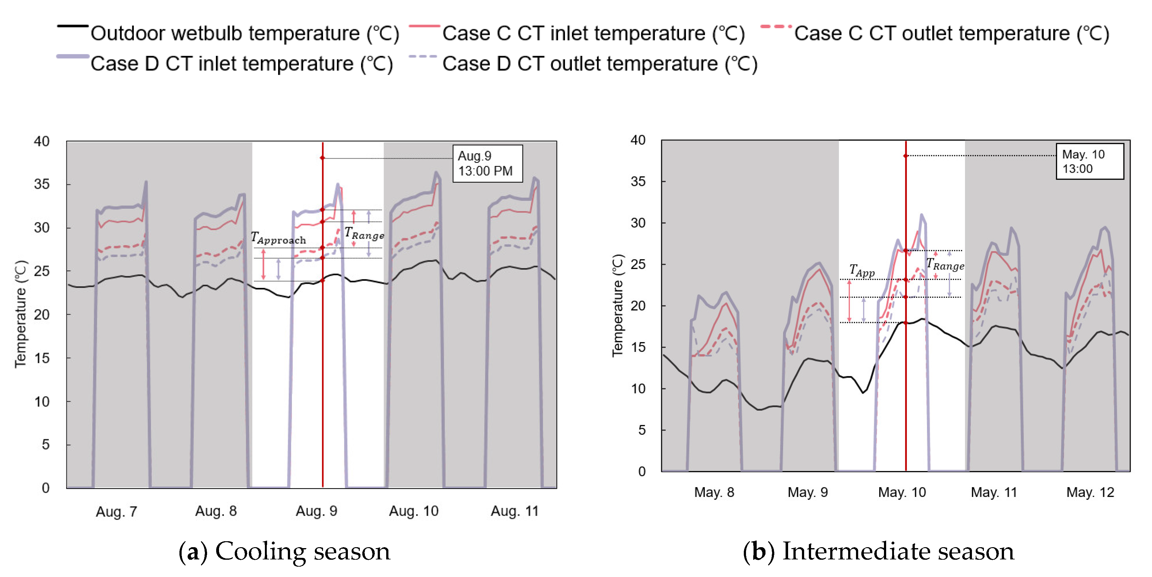
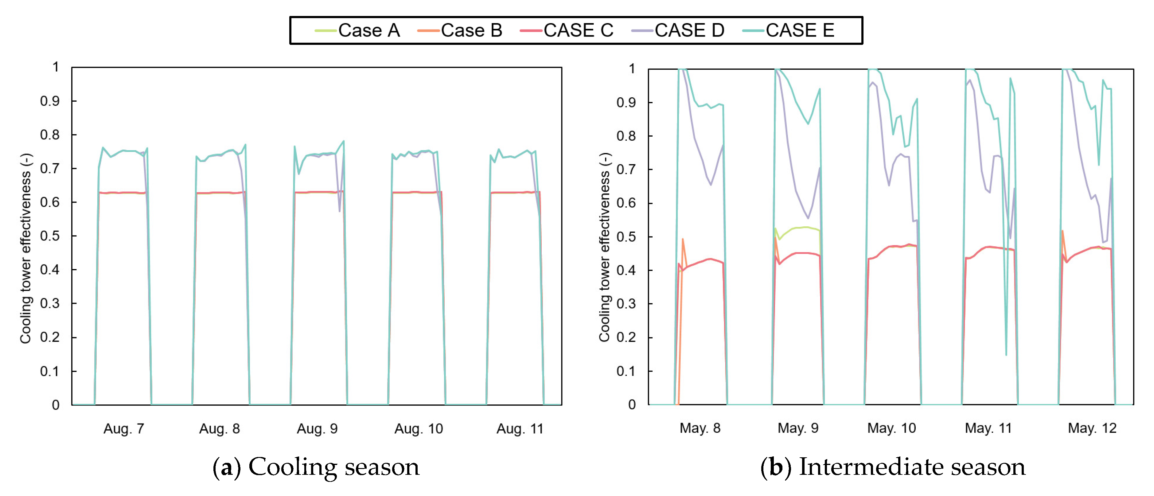
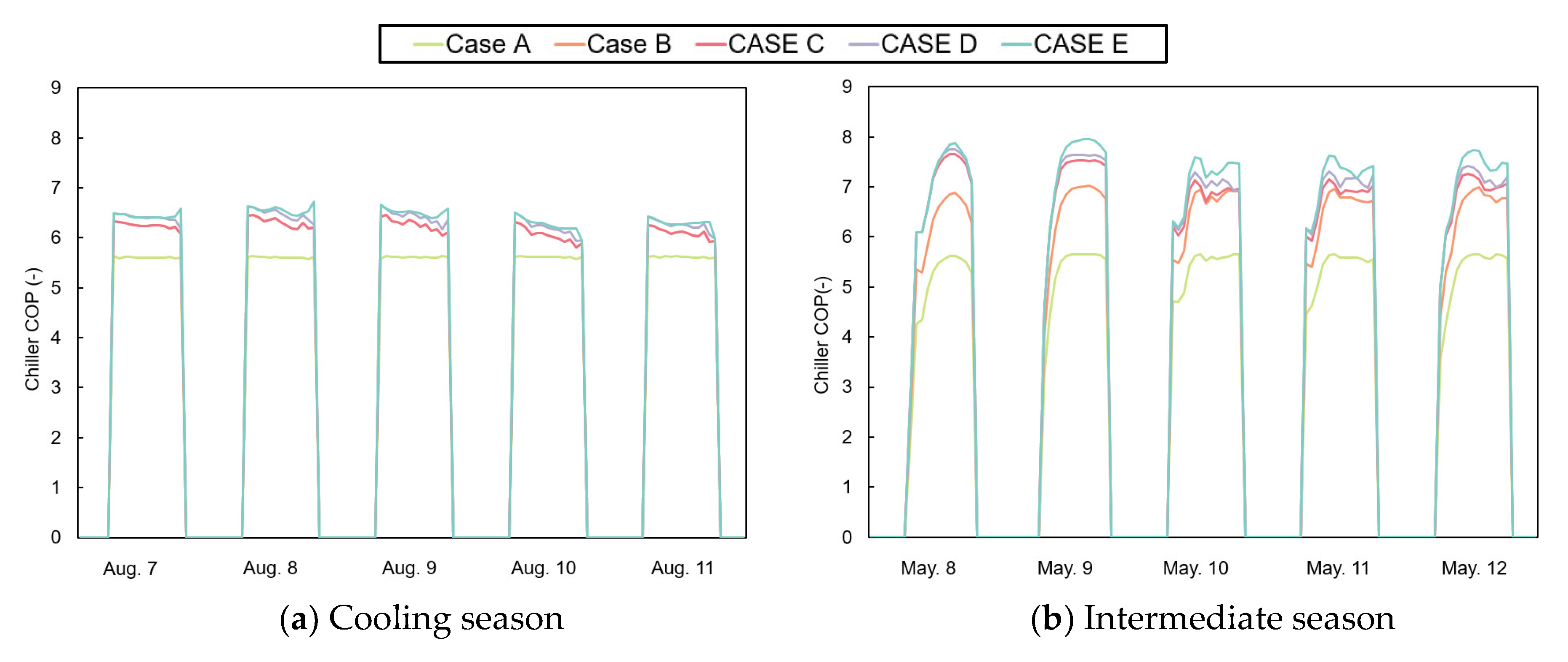
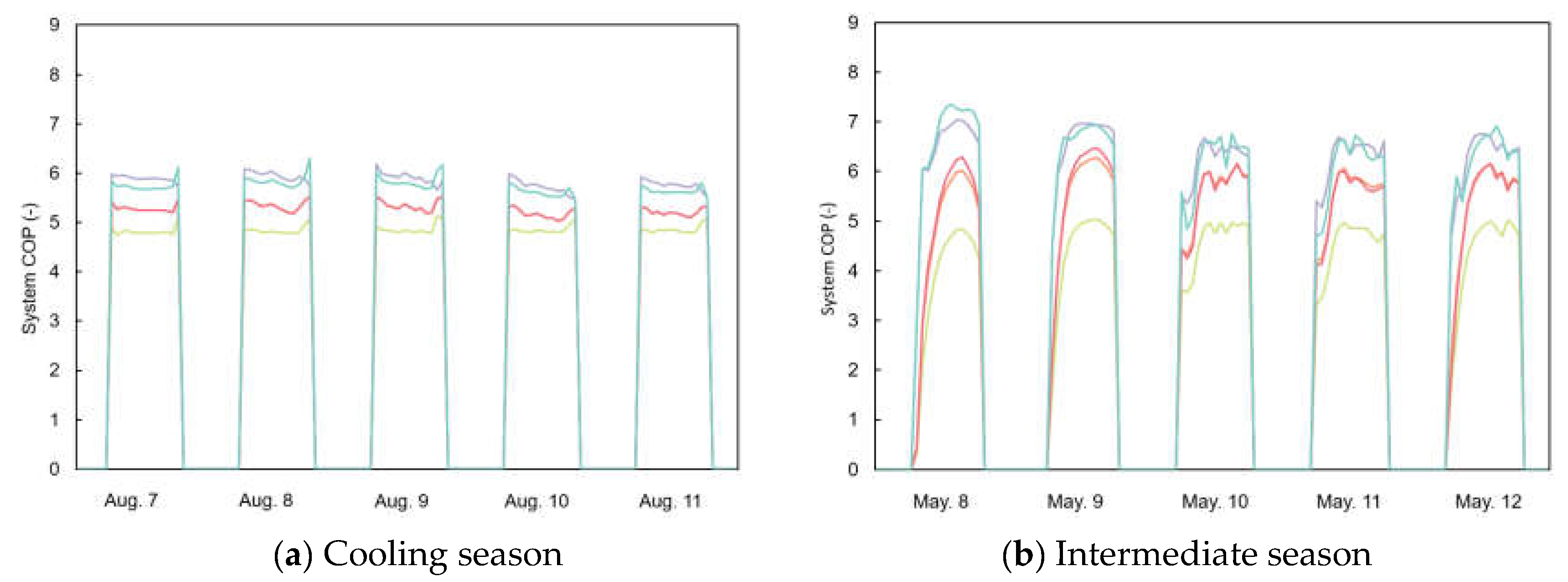
Seasonal Cooling Energy Performance Analysis

Figure 10 shows the energy consumption per component of the cooling system during the representative weeks. The condenser water set temperatures were 32 °C in Case A, 23.9 °C in Case B, and 14 °C in Cases C–E. Although there was a tendency for more energy reduction than Case A, which reflects the general design standards, when the condenser water set temperature was lower, the difference in energy consumption among Cases B–C was minimal, and the only notable energy reduction was achieved in Cases C–E, under the same conditions.

Case B saved 1780 kWh (7.9%) in the representative week of the cooling season and 2182 kWh (21.3%) in the representative week of the intermediate season, compared to Case A. For the cooling season, this result was due to the lower condenser water set temperature (23 °C) than that of Case A (32 °C), leading to a 9.2% reduction in energy consumption by the chillers. The difference in energy consumption was minimal among other components. For the intermediate season, the largest reduction in energy consumption was found in the cooling tower fan at 72.7%, followed by the chiller at 20.7%, and the condenser water pump at 2.2%. The reason for the large reduction in energy consumption of the cooling tower fan was because the system in Case A was configured with on/off control for the cooling tower fan and the condenser water had a fixed flow rate pump, leading to the operation at the rated conditions, regardless of a partial load. On the other hand, when the cooling tower outlet temperature in Case B reached the condenser water set temperature, the cooling tower fan speed was slowed, and the fan air flow rate was reduced. The energy consumption of the chillers was reduced due to the low condenser water set temperature. Despite the condenser water set temperature of Case C being lower than that of Case B, the energy consumption in the representative week of the cooling season was the same, having only a 0.3% difference. During the representative week of the intermediate season, the energy consumption was reduced by 5.3% for the chiller, followed by a 0.3% reduction for the condenser water pump, but the energy consumption of the cooling tower fan increased by 244.1%. This was due to the low condenser water set temperature, which reduced the energy consumption of the chillers, but the cooling tower fan speed had to be maintained at the maximum level to meet the low condenser water set temperature.

Cases A–C focused on the cooling energy reduction according to the change in the condenser water set temperature, whereas Cases C–E aimed to review the energy reduction according to the change in the operation control and system components at the same condenser water set temperature. In Cases D–E, the algorithm detailed in Figure 8 was applied to produce a low approach temperature at the same condenser water set temperature as that of Case C. In Case D, only the algorithm was changed, maintaining the same conditions as those of Case C. The energy consumption in the representative cooling weeks of the cooling and intermediate seasons was reduced by 2131 kWh (10.3%) and 1189 kWh (14.8%), respectively, compared to Case C. The largest energy reduction in the representative week of the cooling season was found in the condenser water pumps at 74.9%, followed by the chillers at 3.3%; and the largest energy consumption in the representative week of the intermediate season was found in the condenser water pump at 80.5%, followed by the cooling tower fans at 14.5%, and the chillers at 4.0%.

Figure 11 shows the cooling tower air and condenser water flow rate in Cases C and D according to the cooling loads. Figure 12 shows the cooling tower inlet and outlet temperatures considering the outdoor air wet-bulb temperature of Cases C and D. When the cooling tower operation control algorithm was applied, the cooling tower fan air and condenser water flow rates were able to be changed, despite the same load conditions, as shown in Figure 11. In Case D, where the algorithm was applied, the cooling tower fan operation was maintained at the maximum air flow in order to operate at the low LGR, and the condenser water flow rate was adjusted according to the cooling tower heat rejection rate. Under the same load, when the condenser water flow rate was reduced, the cooling range became larger, which enabled the production of a low approach temperature. For example, as shown in the white box that is highlighted in Figure 12, the range and approach temperatures of Case C, before applying the algorithm, were 3.0 K and 3.7 K, respectively, while those of Case D were 5.6 K and 2.6 K, respectively; after applying the algorithm at 13:00 p.m. on 9 August, during the cooling season. In addition, the temperature range and approach temperatures of Case C were 3.4 K and 5.1 K, respectively, while those of Case D were 5.5 K and 3.2 K, respectively, as of 13:00 p.m. on 10 May, during the intermediate season. With the application of the algorithm, the temperature range increased by 2.6 K, and the approach temperature decreased by 1.1 K during the cooling season. The temperature range increased by 2.1 K, and the approach temperature decreased by 1.9 K during the intermediate season. The intermediate season could secure a lower approach temperature than the cooling season due to the lower outdoor air wet-bulb temperature and reduced cooling load. Thus, if the LGR value is used as one of the main variables during cooling tower operations, different ranges and approach temperatures can be secured even under the same load conditions. Moreover, the reduction in the condenser water pump power consumption and improvement in chiller efficiency are expected due to the reduction in the condenser water flow rate and approach temperature as the low LGR is maintained in the cooling tower.

In Case E, the system components of the cooling tower used in Case D were changed into an integrated cooling tower. The energy consumption in the cooling season was reduced slightly by 150 kWh (0.8%) compared to that of Case D, but the energy consumption in the intermediate season increased by 209 kWh (3%). The energy consumption in the representative week during the cooling season was reduced by 3.9% in the chiller, but that of the condenser water pump and the cooling tower fan increased by 97.9% and 1.1%, respectively. This was because the energy consumption of the chiller was larger than that of the other components, resulting in a reduction in overall cooling energy consumption. Furthermore, the energy consumption in the representative week during the intermediate season showed that the chillers and condenser water pumps reduced energy consumption by 0.9% and 14.1%, respectively, but the cooling tower fan increased energy consumption by 72.1%. Although the energy consumption of the chiller was reduced due to the effect of the low-temperature condenser water securing a low approach temperature and, as a result, a low LGR due to the simultaneous operation of two cooling tower fans, the energy consumption of the condenser water pump and cooling tower fans increased the system energy consumption. The increase in the pump’s energy consumption was due to the effect of the specifications of the condenser water pump head. Finally, the comparison results with Case A, while conforming to the rated standards of the cooling tower system, demonstrated that Case E had the largest energy reduction in the representative week during the cooling season, 4063 kWh (18.0%), and Case D had the largest energy reduction during the representative week of the intermediate seasons, 3399 kWh (33.1%). In terms of the cooling system components, despite the representative week of the cooling season, Case E energy consumption was reduced by 15.6% in the chiller and 50.0% in the condenser water pump, while the cooling tower fan energy consumption increased by 0.9%. The representative week of the intermediate season (Case D) showed that the condenser water pump had the largest energy reduction, at 80.9%, followed by the chiller at 27.9%, and the cooling tower fan at 19.8%. Thus, the cooling tower sequencing control method should be considered according to the building’s outdoor air and cooling load conditions.

Figure 13 shows the cooling tower effectiveness for Cases A–E in the representative weeks, calculated via Equation (19). As presented in the equation, the cooling tower effectiveness changes according to the NTU and the LGR. Cases A–C had a similar effectiveness, except for outlier periods, as they were operated under conventional conditions, and the mean values in the representative week of the cooling and intermediate seasons were 0.44 and 0.63, respectively. The effectiveness of Case D, where the algorithm was applied, and Case E, where the integrated cooling tower was also applied, were 0.72 and 0.74 during the cooling season and 0.73 and 0.88 during the intermediate season, respectively. Cases D and E cooling tower effectiveness improved by 14.9% and 17.3% during the cooling season and 65.4% and 100.6% during the intermediate season, respectively, compared to Cases A–C. This result indicated that the low LGR operation of the cooling tower improved the cooling tower’s effectiveness.

Figure 14 and Figure 15 show the chiller and system COPs for Cases A–E in the representative week, calculated using Equations (23) and (24), respectively.

$$CO{P}_{Chiller}=\frac{{\dot{Q}}_{Load}}{{\dot{P}}_{Chiller}}=\frac{{\dot{m}}_w\times C_p\times \Delta T}{{\dot{P}}_{Chiller}}$$

(23)

$$CO{P}_{System}=\frac{{\dot{Q}}_{Load}}{{\dot{P}}_{Chiller}+{\dot{P}}_{CT}+{\dot{P}}_{Pump}}$$

(24)

where, $CO{P}_{Chiller}$ is the COP of the chiller, ${\dot{Q}}_{Load}$ is the cooling load, ${\dot{P}}_{Chiller}$ is the electrical power consumption of Turbo chiller, $CO{P}_{System}$ is the COP of the centralized chilled water system, ${\dot{P}}_{CT}$ is the electrical consumption of the cooling tower, and ${\dot{P}}_{Pump}$ is the electrical power consumption of the condenser water pump.

The COP of Case A in the cooling and intermediate seasons were 5.26 and 5.61, respectively, which were reduced by around 13.0% and 7.2% compared to the rated value. Except for the COPs in Cases B and C during the cooling season, the COPs improved from Case B to E. The COP of the chiller in Cases A–C, operated at a conventional LGR, improved by 2.6% during the cooling season and 13.1% during the intermediate seasons due to the change in the condenser water set temperature. However, despite Case B and C having different condenser water set temperatures, the chiller COP in both operations were the same, exhibiting a limitation. In Cases D and E, the algorithm with the low LGR operation was applied (Figure 8). Compared to the rated value, the chiller COP in Cases D and E improved by 5.1% and 6.1% during the cooling season and 14.9% and 17.9% during the intermediate seasons. This was because Case E, where the integrated cooling tower was applied, maintained a lower LGR than that of Case D due to more cooling tower fan operation, thereby securing a lower approach temperature. The COP in Case E, which had the highest chiller COP, improved by 14.3% in the cooling season and 35.4% in the intermediate season, compared to Case A. Except for Cases D and E, which were operated at low LGR conditions, the efficiency of the system COP improved similarly to that of the chiller COP. The chiller COP of Case E in the intermediate season improved by 2.6%, whereas the system COP improvement was minimal, and the chiller and system COPs in the cooling season were reduced by 1.7% and 5.7%, respectively.

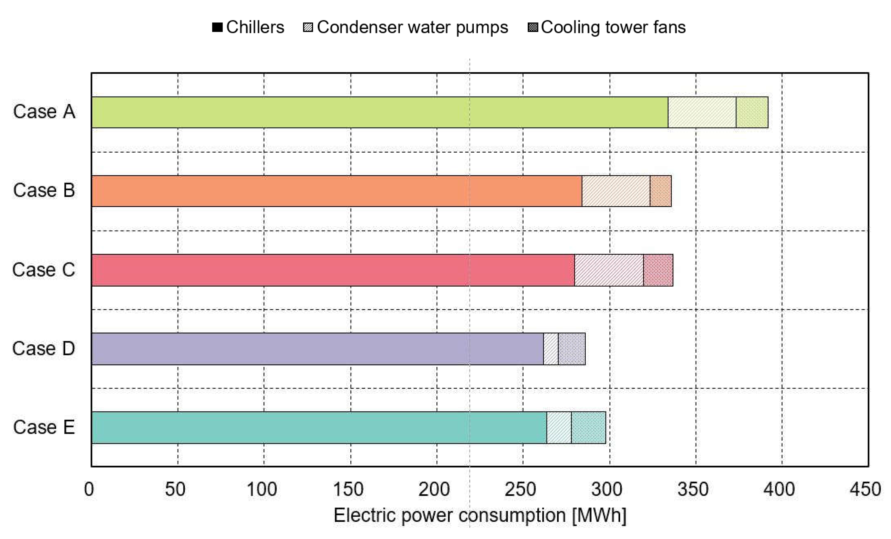
4.3. Annual Cooling Energy Performance Analysis

Figure 16 shows the relationship between the condenser water and outdoor air wet-bulb temperatures for Cases A–E. The data was obtained when the cooling system was operated during the cooling season (June to September) and the intermediate season (April to May, October to November). Some outliers occurred when the cooling system was re-run after operation was interrupted, and others occurred when the outdoor air temperature was too low, in a relative sense. More outliers occurred as cooling time was unstable during the intermediate and cooling seasons. The condenser water set temperatures of Cases A and B were 32 °C and 23.9 °C, respectively, and the condenser water temperatures were maintained, regardless of the outdoor air wet-bulb temperature. In Cases C–E, the condenser water temperatures showed a linear reduction as the outdoor air wet-bulb temperature decreased, exhibiting a data concentration around 14 °C for the condenser water set temperature applying a safety factor. In addition, a lower condenser water temperature could be obtained in the low LGR operation more than in the conventional LGR operation, even with the same condenser water set temperature. Case E, which was operated with the lowest LGR because many cooling tower fans were run at the same time, could reduce the temperature further, by around 1.8 °C on average compared to that of Case C. Thus, the Seoul climate zone, 4A, can operate a central chilled water system with a lower condenser water temperature than 32 °C, which was the rated condition. Furthermore, the approach temperature changed according to the LGR value even in the same range of condenser water set temperatures, through which lower temperature condenser water could be produced.

Figure 17 shows the operation time in relation to the condenser water outlet temperature during the cooling (June to September) and the intermediate seasons (April to May, October to November). The condenser water temperature of 21 °C refers to a range of 20.5–21.4 °C. As shown in Figure 16, Cases A and B are excluded, as their data was distributed densely around their condenser water set temperatures, 32 °C and 23.9 °C, respectively. The data exhibited that 13.6%, 17.2%, and 22.2% of the operations in Cases C–E during the system operation period, including the cooling and intermediate seasons, were operated at the set condenser water temperature of 14 °C. When the cooling tower was operated, as the LGR was lower, a lower condenser water temperature and operation time could be acquired. Moreover, since 58.1%, 67.2%, and 72.4% of the operations in Cases C–E can be secured at a lower range of condenser water temperatures than 23.9 °C of the condenser water set temperature during the entire system operation period, the condenser water set temperature can be lowered to the lower limit of the chiller.

Figure 18 shows the monthly COP of the chiller and system in Cases A–E. Because low-temperature condenser water can be produced according to the low outdoor air wet-bulb temperature in the intermediate seasons (April to May, October to November) compared to that in the cooling season (June to September), both the chiller and the system could secure relatively higher COPs. Accordingly, the production of a low approach temperature is important to achieve additional improvement in cooling system efficiency and energy savings. To do this, low LGR operations are needed. The average chiller COP of Case E, operated at the lowest LGR, was 6.7, a 29.6% improvement, compared to the average chiller COP of 5.2 in Case A, whose cooling tower system was designed with the rated conditions. This was because the compressor power of the chiller was reduced as the low condenser water temperature was produced with low LGR operation. In contrast with the chiller COP, the average system COP of Case D was 6.1, which was 1.2% higher than the 6.0 of Case E; compared to Case A, which had the rated condition, the average system COP improved by 47.4%. The chiller COP of Case E was increased more than that of Case D, but the system COP was reduced due to the increase in the consumption of the cooling tower fans and the condenser water pump energy to secure the lower approach temperature.

Figure 19 shows the annual energy consumption of Cases A–E. The annual energy consumption of the system energy in Case B was reduced by 335.8 MWh (14.3%) compared to that of Case A, and for the components, the cooling tower fan had the largest reduction of 33.5%, followed by the chiller at 14.9%. Since Case A consisted of the cooling tower fan control on/off and a fixed flow rate condenser water pump, it was operated constantly at the rated condition. On the other hand, despite the condenser water set temperature of Case B being low, when it reached the set temperature, the cooling tower fan shut off due to the condenser water pump flow rate control. Despite that, Case C was set to a lower condenser water set temperature, and the system energy increased by 0.8% compared to Case B. This was because the energy consumption of the chiller was reduced by 1.4%, but the energy consumption of the cooling tower fan increased by 39.4% in order to reach the lower condenser water set temperature.

In Case D, the low LGR algorithm operation was applied with the same condenser water set temperature as in Case C. The results revealed that the system energy was reduced by 50.5 MWh, around a 15% savings, and for each component, the condenser water pump had the largest reduction at 78.3%, followed by the cooling tower fan at 8.4%, and the chiller at 6.5%. This was because the lower approach temperature could be secured through low LGR operations, thereby increasing the operation time of the low-temperature condenser water. In addition, the applied algorithm reduced the flow rate of the condenser water and maintained the speed of the cooling tower fan to the maximum before reaching the condenser water set temperature, thereby securing a low LGR. This was the opposite of the cooling tower operations in Case B, and the energy consumption of the cooling tower fan increased by 39.4%. This result indicated that the increase in air flow due to the increase in the cooling tower fan speed was important to the production of low-temperature condenser water securing a low approach temperature. Case E integrated a cooling tower to expand the air flow from the configuration of Case D. However, the system energy increased by 11.95 MWh, which was around 4.2%, compared to that of Case D. Thus, the efficient operation of the individual cooling tower (Case D) showed a better energy performance than the integrated cooling tower (Case E). Finally, when Case A, which reflected the rated standards of the cooling tower system, and Case D, which showed the largest annual energy reduction due to the algorithm application, were compared, the system energy was reduced by 105.8 MWh, which was around 27.0%. The condenser water pump had the largest reduction of 78.5% for each component, followed by the chiller at 21.5% and the cooling tower fan at 15.1%.

5. Conclusions

This study developed a cooling tower operation control algorithm from an LGR perspective. From the LGR perspective, operations may change the condenser water temperature in consideration of the operating efficiency of the cooling tower. Comparing the rated condition to when the low-approach temperature algorithm was applied, the energy savings were 27% per year. The average COP of the chiller and system improved by 27.8% and 47.4%, respectively. In addition, it was found that cooling energy costs were reduced by 15% per year. The average COP of chillers and systems improved by 2% and 23.2%, respectively, after applying the algorithm, even at the same set temperature of the cooling water. This means that the approach temperature can be changed in real-time according to the LGR value of the condenser loop, that is, the operating conditions of the cooling tower, even under the same load conditions and outside air wet bulb temperature. In addition, operation from the LGR perspective can determine the priority of cooling tower fan airflow control and cooling water pump flow control within the condenser loop. Through this, it is possible to solve the low approach temperature manufacturing problem and mitigate low delta-T syndrome on the condenser water loop side.

When the cooling tower is operated with low LGR according to the algorithm developed as a result of this study, it is possible to improve the system efficiency only by applying the control algorithm without the additional high-efficiency devices. Even within the same cooling tower system specification, low LGR can be achieved by reducing the cooling water flow and using max cooling tower fan speed operations. Since the flow rate of the condenser water pump changes according to the load, it is considered that when the cooling water temperature is higher than the set temperature, cooling tower fan airflow control should be prioritized to achieve a low approach temperature.

In previous studies [4,5,18,19,21], low-temperature condenser water was set to a temperature corresponding to the area’s climate conditions; this study found that low-temperature condenser water can be produced down to the lower limit temperature of the chiller in climate zone 4A. Moreover, this study proposed that the LGR, considered in the existing cooling tower design, from the operational viewpoint, can be applied to the installation of a water-cooled chilled water system that uses a cooling tower.

The LGR algorithm application in the cooling tower system (condenser loop) side proposed in this study is the initial step for improving the efficiency of the existing central chilled water systems. To improve efficiency in the central chilled water system, additional studies should be conducted on the air loop side, which is the air-conditioning area, and the plant loop side, in addition to the condenser loop. Thus, the future study will search for the control sequence and efficiency improvement measures of the overall central chilled water system by adding the air and plant loops.

References

1. IEA. The Future of Cooling: Opportunities for Energy-Efficient Air Conditioning. 2018, pp. 1–92. Available online: https://www.iea.org/reports/the-future-of-cooling (accessed on 20 September 2022).
2. Morrison, F. Saving water with cooling towers. ASHRAE J. 2015, 57, 20–33. [Google Scholar]
3. Huang, S.; Zuo, W.; Sohn, M.D. Improved cooling tower control of legacy chiller plants by optimizing the condenser water set point. Build. Environ. 2017, 111, 33–46. [Google Scholar] [CrossRef] [Green Version]
4. Ho, W.T.; Yu, F.W. Improved model and optimization for the energy performance of chiller system with diverse component staging. Energy 2020, 217, 119376. [Google Scholar] [CrossRef]
5. Wang, L.; Lee, E.W.M.; Yuen, R.K.K. A practical approach to chiller plants’ optimization. Energy Build. 2018, 169, 332–343. [Google Scholar] [CrossRef]
6. Tirmizi, S.A.; Gandhidasan, P.; Zubair, S.M. Performance analysis of a chilled water system with various pumping schemes. Appl. Energy 2012, 100, 238–248. [Google Scholar] [CrossRef]
7. Liu, Z.; Tan, H.; Luo, D.; Yu, G.; Li, J.; Li, Z. Optimal chiller sequencing control in an office building considering the variation of chiller maximum cooling capacity. Energy Build. 2017, 140, 430–442. [Google Scholar] [CrossRef]
8. Li, Z.; Huang, G.; Sun, Y. Stochastic chiller sequencing control. Energy Build. 2014, 84, 203–213. [Google Scholar] [CrossRef]
9. Seo, B.M.; Lee, K.H. Detailed analysis on part load ratio characteristics and cooling energy saving of chiller staging in an office building. Energy Build. 2016, 119, 309–322. [Google Scholar] [CrossRef]
10. Goldstein, E.A.; Raman, A.P.; Fan, S. Sub-ambient non-evaporative fluid cooling with the sky. Nat. Energy 2017, 2, 17143. [Google Scholar] [CrossRef]
11. Al-Bassam, E.; Alasseri, R. Measurable energy savings of installing variable frequency drives for cooling towers’ fans, compared to dual speed motors. Energy Build. 2013, 67, 261–266. [Google Scholar] [CrossRef]
12. Sun, J.; Reddy, A. Optimal control of building HVAC&R systems using complete simulation-based sequential quadratic programming (CSB-SQP). Build. Environ. 2005, 40, 657–669. [Google Scholar] [CrossRef]
13. Ma, Z.; Wang, S.; Xu, X.; Xiao, F. A supervisory control strategy for building cooling water systems for practical and real time applications. Energy Convers. Manag. 2008, 49, 2324–2336. [Google Scholar] [CrossRef]
14. Liu, C.W.; Chuah, Y.K. A study on an optimal approach temperature control strategy of condensing water temperature for energy saving. Int. J. Refrig. 2011, 34, 816–823. [Google Scholar] [CrossRef]
15. Yao, Y.; Lian, Z.; Hou, Z.; Zhou, X. Optimal operation of a large cooling system based on an empirical model. Appl. Therm. Eng. 2004, 24, 2303–2321. [Google Scholar] [CrossRef]
16. Zhang, Z.; Li, H.; Turner, W.D.; Deng, S. Optimization of the cooling tower condenser water leaving temperature using a component-based model. ASHRAE Trans. 2011, 117, 934–944. [Google Scholar]
17. Huang, S.; Malara, A.C.L.; Zuo, W.; Sohn, M.D. A Bayesian network model for the optimization of a chiller plant’s condenser water set point. J. Build. Perform. Simul. 2018, 11, 36–47. [Google Scholar] [CrossRef]
18. Kang, W.H.; Yoon, Y.; Lee, J.H.; Song, K.W.; Chae, Y.T.; Lee, K.H. In-situ application of an ANN algorithm for optimized chilled and condenser water temperatures set-point during cooling operation. Energy Build. 2021, 233, 110666. [Google Scholar] [CrossRef]
19. Lee, J.H.; Kim, H.; Song, Y.H. A Study on verification of changes in performance of a water-cooled VRF system with control change based on measuring data. Energy Build. 2018, 158, 712–720. [Google Scholar] [CrossRef]
20. Kim, T.Y.; Lee, J.M.; Yoon, Y.B.; Lee, K.H. Application of Artificial Neural Network Model for Optimized Control of Condenser Water Temperature Set-Point in a Chilled Water System. Int. J. Thermophys. 2021, 42, 172. [Google Scholar] [CrossRef]
21. Thangavelu, S.R.; Myat, A.; Khambadkone, A. Energy optimization methodology of multi-chiller plant in commercial buildings. Energy 2017, 123, 64–76. [Google Scholar] [CrossRef]
22. Singh, K.; Das, R. An experimental and multi-objective optimization study of a forced draft cooling tower with different fills. Energy Convers. Manag. 2016, 111, 417–430. [Google Scholar] [CrossRef]
23. Singh, K.; Das, R. A feedback model to predict parameters for controlling the performance of a mechanical draft cooling tower. Appl. Therm. Eng. 2016, 105, 519–530. [Google Scholar] [CrossRef]
24. Agrawal, A.; Khichar, M.; Jain, S. Transient simulation of wet cooling strategies for a data center in worldwide climate zones. Energy Build. 2016, 127, 352–359. [Google Scholar] [CrossRef]
25. Wen, X.; Liang, C.; Zhang, X. Experimental study on heat transfer coefficient between air and liquid in the cross-flow heat-source tower. Build. Environ. 2012, 57, 205–213. [Google Scholar] [CrossRef]
26. Tomás, A.C.C.; Araujo, S.D.O.; Paes, M.D.; Primo, A.R.M.; da Costa, J.A.P.; Ochoa, A.A.V. Experimental analysis of the performance of new alternative materials for cooling tower fill. Appl. Therm. Eng. 2018, 144, 444–456. [Google Scholar] [CrossRef]
27. Lavasani, A.M.; Baboli, Z.N.; Zamanizadeh, M.; Zareh, M. Experimental study on the thermal performance of mechanical cooling tower with rotational splash type packing. Energy Convers. Manag. 2014, 87, 530–538. [Google Scholar] [CrossRef]
28. Peterson, K.W. Open cooling tower design considerations. ASHRAE J. 2016, 58, 50–54. [Google Scholar]
29. Naphon, P. Study on the heat transfer characteristics of an evaporative cooling tower. Int. Commun. Heat Mass Transf. 2005, 32, 1066–1074. [Google Scholar] [CrossRef]
30. Costelloe, B.; Finn, D.P. Heat transfer correlations for low approach evaporative cooling systems in buildings. Appl. Therm. Eng. 2009, 29, 105–115. [Google Scholar] [CrossRef] [Green Version]
31. Nasrabadi, M.; Finn, D.P. Mathematical modeling of a low temperature low approach direct cooling tower for the provision of high temperature chilled water for conditioning of building spaces. Appl. Therm. Eng. 2014, 64, 273–282. [Google Scholar] [CrossRef]
32. Nasrabadi, M.; Finn, D.P. Performance analysis of a low approach low temperature direct cooling tower for high-temperature building cooling systems. Energy Build. 2014, 84, 674–689. [Google Scholar] [CrossRef]
33. Schwedler, M. Effect of heat rejection load and wet bulb on cooling tower performance. ASHRAE J. 2014, 56, 16–22. [Google Scholar]
34. Seshadri, B.; Rysanek, A.; Schlueter, A. High efficiency ‘low-lift’ vapour-compression chiller for high-temperature cooling applications in non-residential buildings in hot-humid climates. Energy Build. 2019, 187, 24–37. [Google Scholar] [CrossRef]
35. Ha, J.W.; Park, K.S.; Kim, H.Y.; Song, Y.H. A study on Annual Cooling Energy Consumptions Cut-off with Cooling Tower control Change. J. Korean Inst. Archit. Sustain. Environ. Build. Syst. (KIAEBS) 2019, 13, 503–514. [Google Scholar]
36. ASHRAE Standard 90.1-2019; Energy Standard for Buildings Except Low-Rise Residential Buildings. American Society of Heating, Refrigerating and Air-Conditioning Engineers (ASHRAE): New York, NY, USA, 2019.
37. Lawrence Berkeley National Laboratory. Modelica Building Library: Buildings. Fluid.Chillers.Data.ElectricEIR. Available online: https://simulationresearch.lbl.gov/modelica/releases/latest/help/Buildings_Fluid_Chillers_Data_ElectricEIR.html (accessed on 20 September 2022).
38. Gao, D.; Wang, S.; Shan, K.; Yan, C. A system-level fault detection and diagnosis method for low delta-T syndrome in the complex HVAC systems. Appl. Energy 2016, 164, 1028–1038. [Google Scholar] [CrossRef]
39. Rhee, K.N.; Yeo, M.S.; Kim, K.W. Evaluation of the control performance of hydronic radiant heating systems based on the emulation using hardware-in-the-loop simulation. Build. Environ. 2011, 46, 2012–2022. [Google Scholar] [CrossRef]
40. Song, Y.H.; Akashi, Y.; Yee, J.J. A study on the energy performance of a cooling plant system: Air-conditioning in a semiconductor factory. Energy Build. 2008, 40, 1521–1528. [Google Scholar] [CrossRef]
41. Unmet Hours. Question-and-Answer Resource for the Building Energy Modelling Community. Available online: https://unmethours.com/question/35540/condenser-loop-pumpvariablespeed-always-running/ (accessed on 20 September 2022).
42. Unmet Hours. Question-and-Answer Resource for the Building Energy Modelling Community. Available online: https://unmethours.com/question/54977/how-to-simulate-a-variable-speed-condenser-water-pump-in-energyplus/ (accessed on 20 September 2022).
43. EnergyPlus. Input-Output Reference; Department of Energy (DOE): Washington, DC, USA, 2021.
44. Department of Energy (DOE). Python EMS: A Unique EnergyPlus Feature Gets a Serious Upgrade. Available online: https://www.energy.gov/eere/buildings/articles/python-ems-unique-energyplus-feature-gets-serious-upgrade (accessed on 20 September 2022).
45. Stull, R. Wet-bulb temperature from relative humidity and air temperature. J. Appl. Meteorol. Climatol. 2011, 50, 2267–2269. [Google Scholar] [CrossRef] [Green Version]
46. EnergyPlus. Engineering Reference; Department of Energy (DOE): Washington, DC, USA, 2021.
47. ASHRAE. ASHRAE Handbook: HVAC Systems and Equipment; ASHRAE: New York, NY, USA, 2016. [Google Scholar]
48. Statistics Korea. Government Official Work Conference. Available online: http://www.index.go.kr/ (accessed on 20 September 2022).
49. PHIKO (Passive House Institute Korea). Available online: https://climate.onebuilding.org/ (accessed on 20 September 2022).
50. Department of Energy (DOE). Commercial Prototype Building Models. Available online: https://www.energycodes.gov/development/commercial/prototype_models (accessed on 20 September 2022).
51. MOLIT. Building Energy Saving Design Standards; Ministry of Land, Infrastructure, and Transport (MOLIT): Sejong, Korea, 2018. Available online: https://www.law.go.kr/%ED%96%89%EC%A0%95%EA%B7%9C%EC%B9%99/%EA%B1%B4%EC%B6%95%EB%AC%BC%EC%9D%98%EC%97%90%EB%84%88%EC%A7%80%EC%A0%88%EC%95%BD%EC%84%A4%EA%B3%84%EA%B8%B0%EC%A4%80/(2022-52,20220128) (accessed on 20 September 2022).
52. ASHRAE 62.1-2019; Ventilation for Acceptable Indoor Air Quality. American Society of Heating, Refrigerating and Air-Conditioning Engineers (ASHRAE): New York, NY, USA, 2019.
53. MOTIE. Energy Use Rationalization Act; Ministry of Trade, Industry and Energy (MOTIE): Seoul, Korea, 2019.
54. KS B 6270: 2015; Centrifugal Water Chillers. Korean Standards Association (KSA): Seoul, Korea, 2015.
55. KS B 6364: 2014; Performance Tests of Mechanical Draft Cooling Tower. Korean Standards Association (KSA): Seoul, Korea, 2014.
56. Braun, J.E. Methodologies for the Design and Control of Chilled Water Systems. Ph.D. Thesis, University of Wisconsin-Madison, Madison, WI, USA, 1988; p. 434. [Google Scholar]
57. Halasz, B. Application of a general non-dimensional mathematical model to cooling towers. Int. J. Therm. Sci. 1999, 38, 75–88. [Google Scholar] [CrossRef]
58. Jaber, H.; Webb, R.L. Design of cooling towers by the effectiveness-NTU method. J. Heat Transfer. 1989, 111, 837–843. [Google Scholar] [CrossRef]
59. Braun, J.E.; Klein, S.A.; Mitchell, J.W. Effectiveness models for cooling towers and cooling coils. ASHRAE Trans. 1989, 95, 164–174. [Google Scholar]
60. Soylemez, M.S. Theoretical and experimental analyses of cooling towers. ASHRAE Trans. 1999, 105, 330–337. [Google Scholar]
61. Popp, M.; Rogener, H. Calculation of cooling process. In VDI-Warmeatlas; Springer: Berlin/Heidelberg, Germany, 1991; pp. Mi 1–Mi 15. [Google Scholar]
62. Khan, J.R.; Zubair, S.M. An improved design and rating analyses of counter flow wet cooling towers. J. Heat Transf. Trans. ASME 2001, 123, 770–778. [Google Scholar] [CrossRef]
63. Merkel, F. Evaporative cooling. Z. Verein. Deutsch. Ingen. (VDI) 1925, 70, 123–128. [Google Scholar]
64. Chang, C.C.; Shieh, S.S.; Jang, S.S.; Wu, C.W.; Tsou, Y. Energy conservation improvement and ON-OFF switch times reduction for an existing VFD-fan-based cooling tower. Appl. Energy 2015, 154, 491–499. [Google Scholar] [CrossRef]
65. Li, J.; Li, Z. Model-based optimization of free cooling switchover temperature and cooling tower approach temperature for data center cooling system with water-side economizer. Energy Build. 2020, 227, 110407. [Google Scholar] [CrossRef]
Figure 1. Comparison of typical temperature (a) nominal-condition and (b) proposed low-LGR.
Energies 15 07327 g001
Figure 2. Mollier diagram with low-condenser water temperature.
Energies 15 07327 g002
Figure 3. Study flow chart.
Energies 15 07327 g003
Figure 4. The diagram of the whole energy efficiency improvement strategy.
Energies 15 07327 g004
Figure 5. Conventional cooling tower (Case A, B, C, D).
Energies 15 07327 g005
Figure 6. Integrated cooling tower (Case E).
Energies 15 07327 g006
Figure 7. Cooling tower control algorithm for low approach temperature.
Energies 15 07327 g007
Figure 8. Cooling and intermediate season outdoor air condition in Seoul (Climate zone 4A). (a) Cooling and intermediate season outdoor dry and wet-bulb temperature. (b) box plot example.
Energies 15 07327 g008
Figure 9. COP of water-cooled chiller.
Energies 15 07327 g009
Figure 10. Weekly system energy consumption for Case A–E.
Energies 15 07327 g010
Figure 11. Weekly cooling tower air and water flow rate for Case C and D.
Energies 15 07327 g011
Figure 12. Weekly range and approach temperature for Cases C and D.
Energies 15 07327 g012
Figure 13. Weekly cooling tower effectiveness for Case A–E.
Energies 15 07327 g013
Figure 14. Weekly chiller COP for Case A–E.
Energies 15 07327 g014
Figure 15. Weekly system COP for Case A–E.
Energies 15 07327 g015
Figure 16. Relation between condenser water and outdoor wet-bulb temperature for Case A–E.
Energies 15 07327 g016
Figure 17. Annual operation hour of condenser water temperature for Case C–E.
Energies 15 07327 g017
Figure 18. Monthly COP for Case A–E.
Energies 15 07327 g018
Figure 19. Annual system energy consumption for Case A–E.
Energies 15 07327 g019