Article

Effect of Temporal Variation in Chemical Composition on Methane Yields of Rendering Plant Wastewater

School of Engineering and Built Environment, Nathan Campus, Griffith University, Brisbane, QLD 4111, Australia
*
Author to whom correspondence should be addressed.
Energies 2022, 15(19), 7252; https://doi.org/10.3390/en15197252
Submission received: 8 September 2022 / Revised: 28 September 2022 / Accepted: 28 September 2022 / Published: 2 October 2022
(This article belongs to the Special Issue Biomass Wastes for Energy Production 2023)

Abstract

:
The effect of temporal variation in chemical composition on methane yields of rendering plant wastewater was studied in batch experiments at 37 °C. In total, 14 grab samples were collected from Monday through Friday (Day 1 to 5) from a rendering plant located in Queensland, Australia. Each day, three samples were collected: early morning (S1), midday (S2) and afternoon (S3). Chemical analyses showed that a significant different in total solids (TS), volatile solids (VS), and chemical oxygen demand (COD) was noticed among the samples. TS content ranged from 0.13% to 1.82% w/w, while VS content was between 0.11% and 1.44% w/w. Among the samples, S2 of Day 3 had the highest COD concentration (10.5 g/L) whilst S1 of Day 1 had the lowest COD (3.75 g/L) and total volatile fatty acid (VFA) concentration (149.1 mg/L). In all samples, acetic acid was the dominant VFA and accounted for more than 65–90% of total VFAs. Biochemical methane potential studies showed that the highest methane yield of 270.2 L CH4/kgCODadded was obtained from S3 of Day 3. Whilst the lowest methane yield was noticed for S1 of Day 1 (83.7 L CH4/kgCODadded). Results from kinetic modelling showed the modified Grompetz model was best fit than the first order model and a large variation was noticed between the experimental and the modelled data. Time delay ranged from 2.51 to 3.84 d whilst hydrolysis constant values were close to 0.21 d−1. Thus, the study showed that chemical composition of incoming feed to a biogas plant varies throughout the week and is dependent on the chemical composition of organic materials received and the amount of steam used for rendering process.

1. Introduction

Demand for meat products has increased consistently over the past decade due to population growth, urbanization, and dietary shifts. Global meat production has expanded over the past two decades, and it is expected to reach a consumption of 377 Mt by 2031 [1]. Australia’s meat industry has grown consistently over the past decade and is considered as one of the global leaders in meat exports. According to the Australian red meat and livestock industry (MLA), Australia is the first and second-largest exporter of sheep and beef meat in the world, respectively [2]. Nevertheless, this industry has also been recognized as an extensive energy and resource-intensive industry. The environmental protection authority (EPA) in Australia realized that effluent management at animal processing facilities is a major environmental issue owing to high levels of organics viz., fats, oils and grease (FOG), classifying it as high-strength wastewater [3]. Australian red meat processing facilities consume on an average 7.92 kL/t hot standard carcass weight (HSCW) of water and discharge around 6.5 kL/t HSCW of wastewater after processing [4].
The rendering process contributes to more than 50% of the organic and nutrient load of the effluent obtained in animal processing facilities [4]. The chemical oxygen demand (COD) content in wastewaters ranges from 4000 to 10,000 mg/L, with FOG being the primary organic component of rendering wastewaters (RWW) [5]. The current treatment of the RWW involves primary and secondary treatments [6]. Anaerobic treatment is a popular and proven method in management of meat industry wastewaters due to the effective organic matter removal and significant renewable energy generation in the form of methane [7]. In Australia, in areas with land availability, covered anaerobic lagoons (CAL) are the most commonly used technology for treating meat industry wastewaters due to their simplicity in building and operation, plus low capital cost [8]. The aim of the effluent treatment is to reduce the nutrients, organic matter, and FOG and to obtain an effluent that could be used for irrigation within the agricultural field or dispose into sewage.
Several issues have been identified in the treatment of meat industry wastewater by using CAL technology. These include organic and hydraulic overloading with a reduction in treatment efficiency [9,10]; formation and accumulation of crust and effective volume loss [11], and infrastructure damage [12]; and reduction in biogas yields [13,14]. The above identified issues are mainly attributed to the nature and composition of wastewater, which significantly varies from one processing facility to another [15].
There are notable studies in the literature investigating the composition of effluents from different meat processing facilities in Australia [11] and worldwide [16]. The difference in parameters is identified when treating different meat products in the meat processing industries [14,17,18,19]. However, there is no previously published work on the temporal variation in the abattoir wastes received by rendering plants and its impact on the chemical composition of wastewaters and subsequently on the methane composition and yields. Thus, the aim of the present study is to evaluate the effect of temporal variation in chemical composition of abattoir wastes received from Monday through Friday by a rendering plant on its effluent wastewaters (RWW) and methane yields. The results obtained from this work will facilitate in planning the type of abattoir wastes to be received at the rendering plant, daily amounts of water and chemical use in cleaning the rendering plant, designing storage tanks and biogas plants with buffer tanks and/or adjust the organic loading rates (OLR) to biogas plant to maintain process stability and methane yields.

2. Materials and Methods

2.1. Substrate and Inoculum

RWW was collected from a rendering facility (A J Bush & Sons) in Queensland, Australia. The plant operates from Monday to Friday and receives organic waste by-products from red-meat and poultry abattoirs located in south-east Queensland. Materials received in the facility were segregated into five different lines and subject to rendering according to the scheduled day for each line. Rendering process was carried out at 130 °C for 30 min and 20 bars. Thereafter, rendered material is separated into solid and liquid fractions. Solid fraction is sold as dog food and/or organic fertilizer. On the other hand, the liquid fraction is used as feedstock for biogas production. To examine the temporal variation in the chemical composition of the RWW, samples were collected three times per day (morning, S1, midday, S2 and afternoon, S3) on five consecutive weekdays. Rendering facility operates on Fridays until noon, consequently only two samples were obtained on that day. In total, 14 samples were collected and stored at 4 °C immediately to prevent further degradation of organic matter.
Anaerobically digested material from a full-scale biogas plant treating waste activated sludge and primary sludge from sewage treatment plant (Queensland Urban Utilities, Brisbane, Australia) was used as inoculum. The inoculum was degassed by incubating at 37 °C for a week. Degassed inoculum was analysed for the chemical parameters such as pH, ammonium-nitrogen (NH4-N) and volatile fatty acids (VFA) to validate the optimal composition of inoculum as outlined elsewhere [20,21].

2.2. Experimental Set-Up

Biochemical methane potential (BMP) of RWW was performed in batch experiments as per the protocol described elsewhere [20,22]. Briefly, BMP test was carried out in 160 mL glass serum bottles with a working volume of 100 mL. To each assay, 90 mL of inoculum was transferred. RWW was added to achieve a designed inoculum to substrate ratio (ISR) of 4 on COD basis. pH was adjusted to 7.5 by using 3 M sodium hydroxide (NaOH). Assays were sealed with butyl rubber stoppers and aluminum crimps. Sealed assays were then flushed with pure N2 (99%) for five minutes to create anaerobic conditions. Assays with inoculum only were used as controls. Methane produced in control assays was determined and was subtracted from the sample assays. Prepared assays were incubated statically at 37 °C. Methane production and its composition were measured at regular intervals. The experiment was terminated when the variation in methane production was less than 5% for three consequent measurements.

2.3. Kinetic Modelling

The hydrolysis rate constant (Khyd) and lag phase of methane production in different assays were estimated by using the first-order kinetic model Equation (1) and the Gompertz equation model Equation (2) as described elsewhere [23]
B(t) = Bo [1 − e(−khyd ∗ t)]
B(t) = Bo (−e[(Rmax ∗ e)/Bo (λ − t) + 1])
where B(t) is the cumulative methane yield (L CH4 kg−1CODadded), Bo is the maximum specific methane yields (L CH4 kg−1CODadded), Rmax is the maximum specific production rate (L CH4 kg−1 CODadded d−1), tlag is the lag phase (d), khyd constant of hydrolysis (d−1). The Solver tool of Microsoft Office Excel® was used to fit the data in the kinetic model.

2.4. Analitical Methods

Total solids (TS) and volatile solids (VS) were determined according to the Standard Methods [24]. pH was measured immediately by using a pH meter (OHAUS starter300). Total chemical oxygen demand (TCOD) and soluble chemical oxygen demand (SCOD) were determined by the photometric method with the MERK Spectroquant COD Cell test and spectrophotometer Move 100 (Merck) as described elsewhere [25]. Volatile fatty acids (VFAs) were determined by using a Gas Chromatograph (Agilent technologies 789A, Santa Clara, CA, USA) fitted with a flame ionisation detector and Agilent DB-FFAP column [25]. Ammonium nitrogen (NH4-N) was analysed by using Lachat QuikChem 8500 Series 2 Flow Injection Analyser (FIA) in accordance with the established techniques [26]. Total Kjeldahl phosphorus (TKP) and total Kjeldahl nitrogen (TKN) were determined by using an inductivity coupled plasma-optical emission spectroscopy (PerkinElmer ICP-OES Optima 7300DV instrument) as described elsewhere [27]. Total carbon (C) and nitrogen (N) content were measured by using a stable isotope analyser (Sercon Hydra 20–22) and using the method described elsewhere [28]. The biogas composition was analysed by using a gas chromatograph (Shimadzu GC-2014) as per the protocol described elsewhere [29].

2.5. Calculations

The cumulative methane volumes of the studied samples were calculated by summing the methane volumes measured at each sampling time by monitoring the headspace pressure. Biogas was released from the assays when the pressure in the headspace has reached a certain threshold pressure as per Equation (3) [30]
VCH4-STP = [Vheadspace ∗ (Pheadspace/PSTP) ∗ (TSTP/T)] ∗ [%CH4-wet ∗ (1 − (Pvap/(Pambient + Pheadspace))]
In Equation (3) VCH4-STP is the volume of the methane produced by the assay, Vheadspace is the glass serum bottles headspace volume Pheadspace is the manometric pressure measured in the headspace, PSTP and TSTP and are biogas pressure and temperature under standard conditions (1013.25 mbar; 273.15 K), T is the experimental temperature condition (310.15 K). The methane content in biogas measured using gas chromatography is %CH4-wet, and Pvap and Pambient are the vapor pressure of water and ambient pressure at assay temperature.
The cumulative methane yields produced in each assay in terms of CODadded were calculated by using Equation (4), where VCH4-STP and VCH4-STP-control are the volume of methane produced by the sample and control assay, respectively. The gCOD sample represent the amount of COD added per sample in the test.
Cumulative methane yield = [(VCH4-STP) − (VCH4-STP-control)/gCOD sample]
The experimental COD removal efficiency was calculated by using Equation (5), where CODo and CODf represent the initial and final COD, respectively [31].
CODremoval (%) = [(CODo − CODf)/CODo] ∗ 100

2.6. Statistical Analysis

Chemical analysis and biomethane potential test results are presented as the average values ± standard error of the mean from the three replicates used in the study. To evaluate the effect of temporal variation, chemical composition, and methane potential of the 14 studied samples were assessed for significance using one-way ANOVA or t-test with a Tukey’s post hoc test at a significance level of 0.05 by using IBM SPSS Statistics® software.

3. Results and Discussion

3.1. Temporal Variation in Chemical Composition of Rendering Plant Wastewater

The temporal variation in chemical composition of the studied RWW samples is presented in Table 1. Results showed that TS content in the samples ranged from 0.13 to 1.82% w/w. The sample S3 of Day 2 reported the highest TS and VS values of 1.82% and 1.44%, respectively. Overall, a VS/TS ratio of >0.70 was noticed in the samples across the five-day sampling period indicating that the studied samples had high organic matter and can be considered as good feedstocks for methane production [32]. This was also evident from the COD content in the samples, which ranged from 3747 to 9047.9 mg/L (Table 1). A significant variation in COD across the five days was noticed. For Days 1, 2, and 4, S3 had the highest COD content compared to S1 or S2 samples, while S2 sample had the highest COD among Day 3 and 5 samples. These COD values are comparable to the values reported for RWW in a study from the Czech Republic [33]. For instance, COD values ranging from 4333 to 9000 mg/L were reported in the above study [33]. However, no such trend was noticed for NH4-N and phosphorus (PO4-P) in the studied samples. Ammonium concentration fluctuated from a low 42.9 mg/L (S1 of Day 1) to the maximum value of 71.3 mg/L (S1 of Day 2). Similarly, PO4-P concentration ranged from 33.1 to 76.3 m/L. Interestingly, S1 of Day 2 accounted for the highest concentration of NH4-N and PO4-P among the studied samples. Similar NH4-N concentrations of 58.9 mg/L were also reported for RWW in the United States [5].
Organic content in RWW was mostly produced by short-chain fatty acids, with acetic acid as the predominant species [33]. Total VFA content in the samples ranged from a low 149.1 mg/L to 455.4 mg/ L (Table 1). Within each day, total VFA content increased from S1 to S3. This trend was noticed across all five days of sampling. Among the studied samples, S3 of Day 3 sample had the highest VFA of 455.4 mg/L, with acetic acid accounting for 91.84% of total VFA (Table 1). Conversely, S1 of Day 1 had the lowest VFA concentration of 149.1 mg/L (65.12% of total VFA being acetic acid).
One-way ANOVA results revealed that there is a statistically significant difference (p ≤ 0.001, Table 1) in chemical composition across all samples. A Tukey post hoc test was also conducted to evaluate whether there is any significant difference in chemical composition within each day. Results showed that a significant difference in TS and VS content was noticed among the S1–S3 samples (p ≤ 0.001). A significant variation in COD, total VFA, and NH4-N concentrations was also noticed (p ≤ 0.0001) indicating that there is a temporal variation in the chemical composition of RWW during the studied period. On the other hand, no significant difference (p ≥ 0.05) was noticed for TKP content, except for Day 4 (p ≤ 0.004). Such differences in chemical composition in daily samples are associated with the variation in abattoir waste materials received by rendering facilities and also attributed to the presence of non-edible residues such as skinning residuals, blood content and intestinal components, which is dependent on the type of animal slaughtered at the abattoirs [16,34].

3.2. Batch Experiments

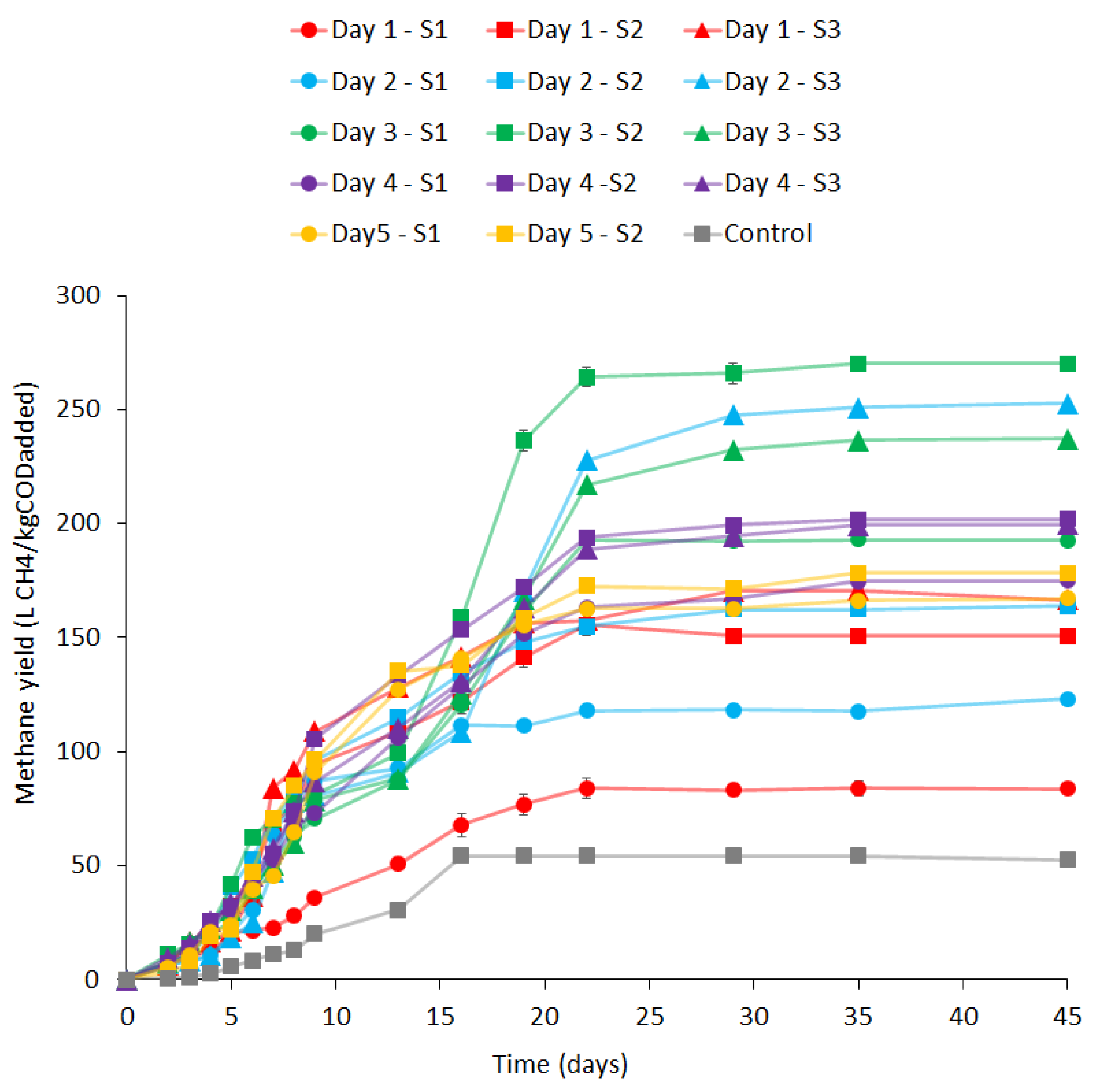
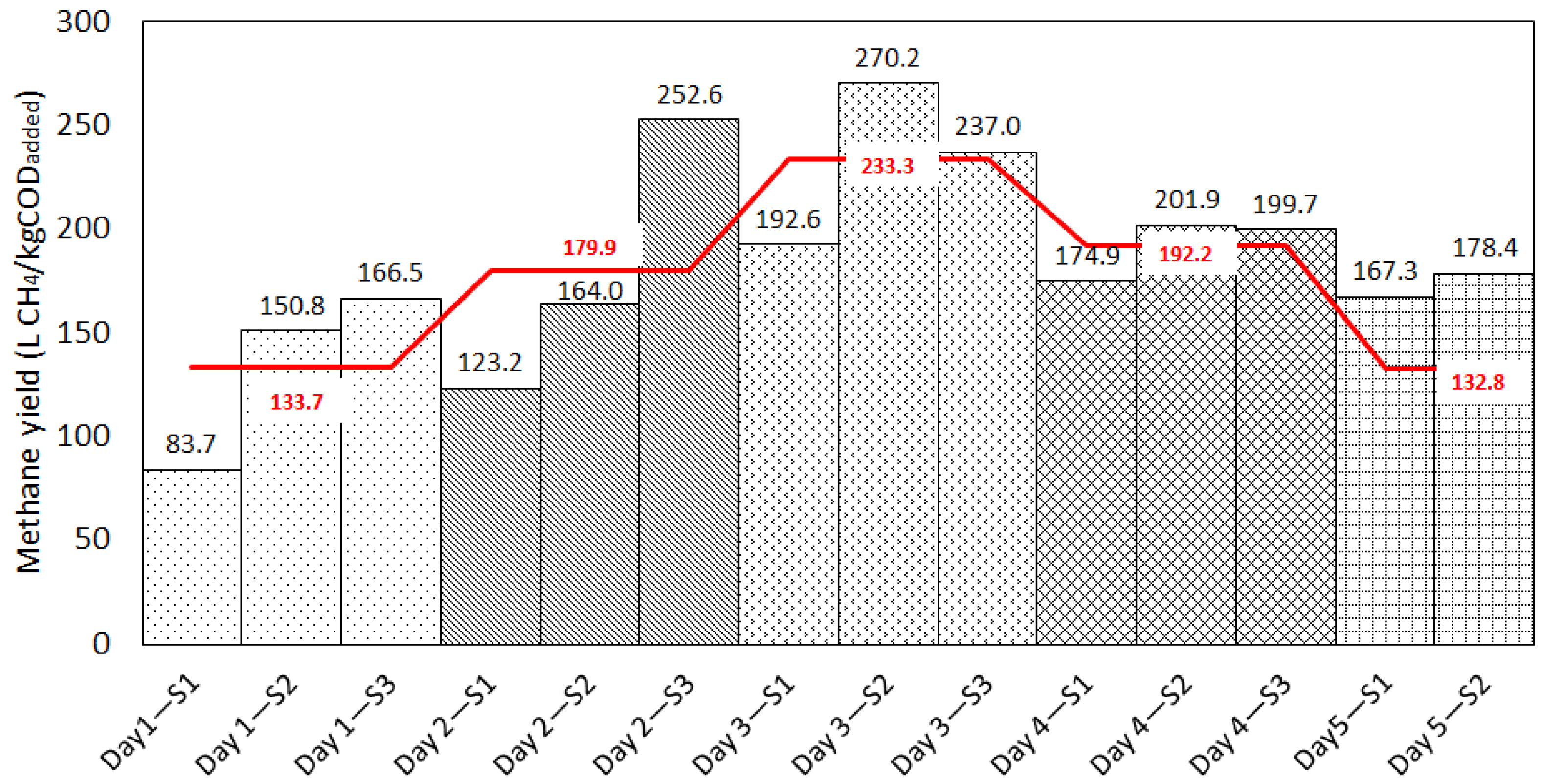
3.2.1. Effect of Temporal Variation in Chemical Composition on Methane Yields from Rendering Wastewater

Cumulative methane yields obtained for each sample collected from Monday through Friday are presented in Figure 1 Methane production rates and methane yields varied across the samples (Figure 2). This variation is attributed to the variation in the chemical composition of the samples (Table 1).
Methane production started in all samples but with a lag phase of around three to five days (Figure 1). Although methane production was low in the first few days, a steady increase in methane production was noticed after second day of incubation. Overall, 80% of the methane was produced by Day 16, with the highest daily methane production obtained for S2 on Day 3 (77.27 L CH4/kgCODadded). Thereafter, a decrease in methane production was noticed for most of the samples leading to flattening of the cumulative methane production by Day 20 (Figure 1). RWW components, such as fats, oils and grease (FOG), have been associated with inhibition of biogas generation due to the accumulation of long chain fatty acids (LCFAs), which form during the hydrolysis stage [5]. LCFA components tend to bond to the sludge microbes’ surface, limiting the mass transfer between the active bacteria and the media and inhibiting acetoclastic and hydrogenotrophic methanogens [11]. For RWW, accumulation of palmitic acid has been reported as the cause of temporal inhibition of acetoclastic methanogenesis; however, with adequate growth of syntrophic bacteria, inhibition is reversed and biogas production can resume [5].
At the end of 45 days of incubation, cumulative methane yields for the samples ranged from 83.7 to 270.2 L CH4/kgCODadded (Figure 1). An upward trend in the methane yields was found when comparing samples within the same day. The lowest methane yields were obtained for sample S1 across Day 1 to Day 5 (Figure 2). It is associated with the low chemical strength of S1 samples (early morning) received on each day (Table 1) suggesting that the wastewaters were received from a nearby abattoirs or butchers dealing with animals that are small to medium standard carcasses weight.
Results showed that there was a clear relation between COD concentration in the RWW and the obtained methane yields, with higher methane yields noticed for samples with higher COD values (Figure 2 and Table 2). Sample S2 of Day 3 had the highest COD concentration (10,469.1 mg/L) and resulted in producing the highest methane yield (270.2 L CH4/kgCODadded). It suggests that this sample had high content of readily biodegradable COD that could be easily converted into biogas. On comparison with Day 3 samples, methane yields from Day 1 and Day 2 were lower by 42.7% and 22.9%, respectively. This was evident from the significant difference in the COD values. Day 1 and 2 samples had 54% and 84% lower COD content than the values noticed for Day 3 (Table 1).
An opposite effect on methane yields was noticed with the concentration of NH4-N in the studied samples. Despite that no inhibitory concentration was found in studied wastewaters, as discussed in previous sections, a trend of lower methane yields with higher concentrations of NH4-N was found. First sample collected from each studied day, except from Day 4, reported the highest NH4-N concentration (Table 1) and at the same time reported the lowest methane yields among the samples collected on each day (Figure 1). For instance, NH4-N concentration was 59.9 mg/L and 56.9 mg/L for S1 and S2 on Day 5, respectively, with the former producing 6.22% less of methane yield than the latest. Among the samples tested, highest methane yield of 270.2 L CH4/kgCODadded was obtained for sample S2 of Day 3 (Figure 2). The methane yield obtained in the present study was lower than the yield of 320 L CH4/kgCODadded reported in the literature [5]. The discrepancy between the yield obtained in the present study and with the methane yields reported in the literature can be attributed mainly to the differences in the chemical composition of the studied wastewaters and conditions used in the BMP test. For instance, Xie et al. (2021) reported the methane yields of RWW obtained from a plant treating only poultry residues, while the RWW used in this study came from a rendering plant dealing with meat and poultry by-products from abattoirs, retail butcher shops and meat processors into high grade protein meals and tallow. The residual wastewater is then used for biogas production in a CAL. Subsequently, the produce biogas is used for cogeneration in a combined heat and power plant.
The lowest methane yield of 83.7 L CH4/kgCODadded noticed for sample S1 on Day 1 was probably due to the dilution of the RWW with the wash water containing detergents and disinfectants used during the downtime period when cleaning activities are carried out. Detergents or disinfectants used during cleaning and washing activities can remain in the resultant wastewaters and even last in some equipment and/or pipes transporting wastewater. Small amounts of detergents were known to cause an inhibitory effect on the methanogens thereby affecting the anaerobic digestion process [35,36]. For instance, a decrease in methane yields from 0.36 to 0.16 L CH4/kgCODadded was noticed when the detergent concentration increased from 1 to 10mL/L [37].
The one-way ANOVA results showed that a statistically significant difference (p ≤ 0.001) in cumulative methane yields was noticed across all samples. Further, Tukey post hoc test was performed to evaluate whether there is any significant difference within the day samples. A significant difference in methane yields was noticed in the samples collected on the same day (p ≤ 0.001). Among the 14 studied samples, which results in 182 different combinations between samples, only 5 group of samples where statistically significant: S3—Day 1 and S2—Day 2 (p = 0.84); S3—Day 1 and S1—Day 5 (p = 0.99); S2—Day 2 and S1—Day 5 (p = 0.47); S1—Day 4 (p = 0.41); S2 and S3—Day 4 (p = 0.92). The results thus reveal that temporal variation in chemical composition of wastewater at the studied rendering plant can significantly affect the methane yields.

3.2.2. Chemical Composition of the Digestates

Total VFA concentration in the digestates of the samples was between 15.66 and 18.31 mg/L (Table 2). Acetic acid was the major VFA component and accounted for more than 70% of the total VFAs. Iso-butyric acid, iso-valeric and hexanoic acid were not detected. This result is in accordance to the result reported in the literature [5]. The highest acetate concentration of 13.1 mg/L was noticed in S2 of Day 3 (Table 2). Interestingly, this sample also had the highest COD removal (Table 1). The high residual acetate in some of the samples indicate that some of the components from the RWW had affected the acetoclastic methanogens [11,38,39].
Samples reported a COD degradation higher than 60% (Table 2). There was a clear trend in which higher percentage of degradation were associated with the highest methane yields obtained. As expected, S2—Day 3 had the highest biodegradability (80.79%) and thus resulted in the highest methane yields (Table 2). Conversely, Day 1 sample had the lowest COD conversion among the sampled days. It can be associated with the readily biodegradable COD concentration as discussed in previous sections. COD removal rates obtained in this study are similar to the ones reported in the literature for RWW [5].
TKN concentrations ranged from 0.14 to 0.40 mg/kg in the digestate obtained after digestion process. All samples showed a lower concentration of TKN than the initial concentration in the feed suggesting that ammonification of proteins had not occurred during the anaerobic digestion process [40].
Among the sample tested, acetic acid was the major VFA accounting for more than 65% in all cases. There was a significant reduction in VFA concentrations when values were compared between feed and digestate. Such decrease is associated with the VFA consumption by acetogenic bacteria during the anaerobic degradation as discussed in the literature [41].

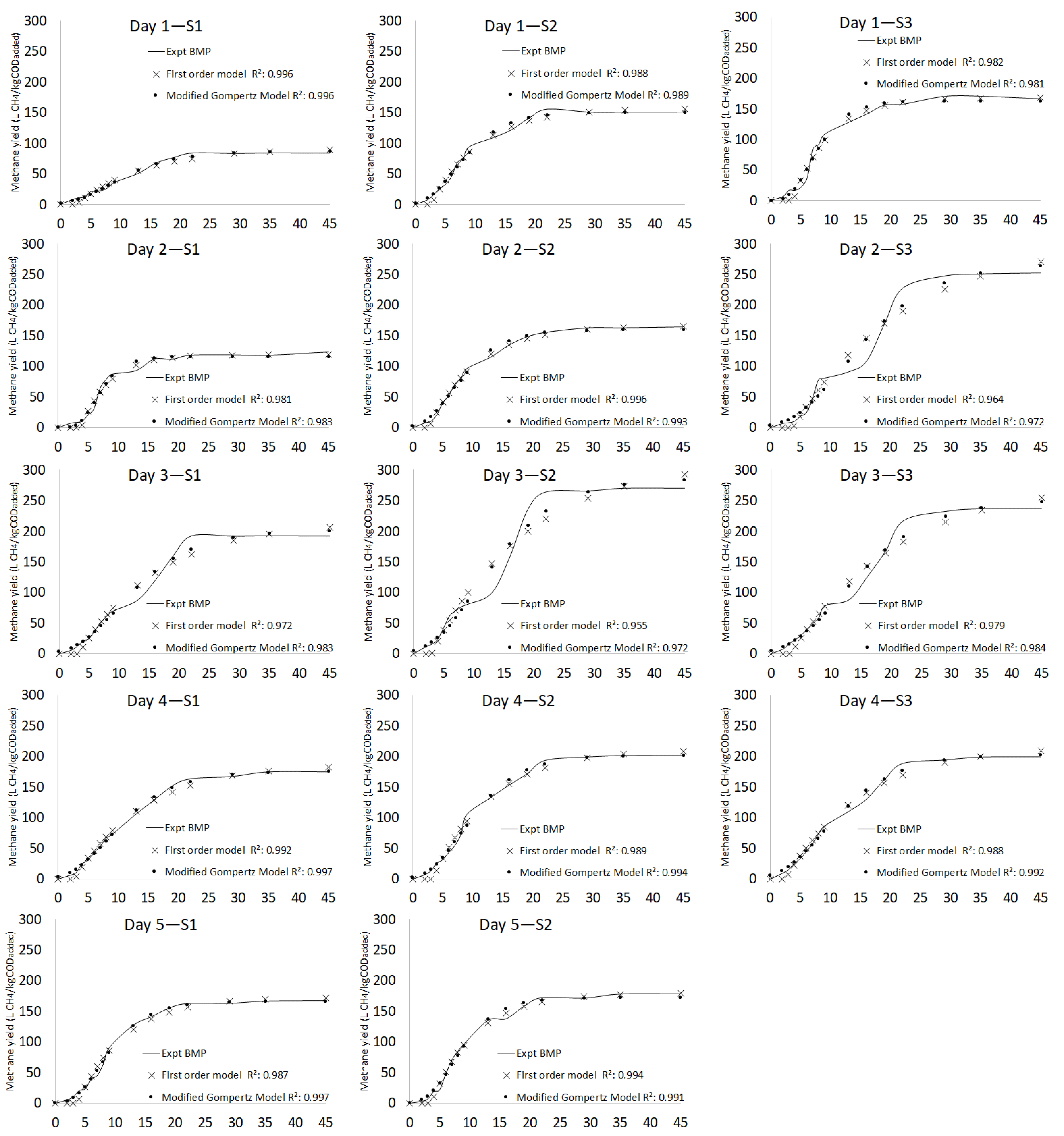
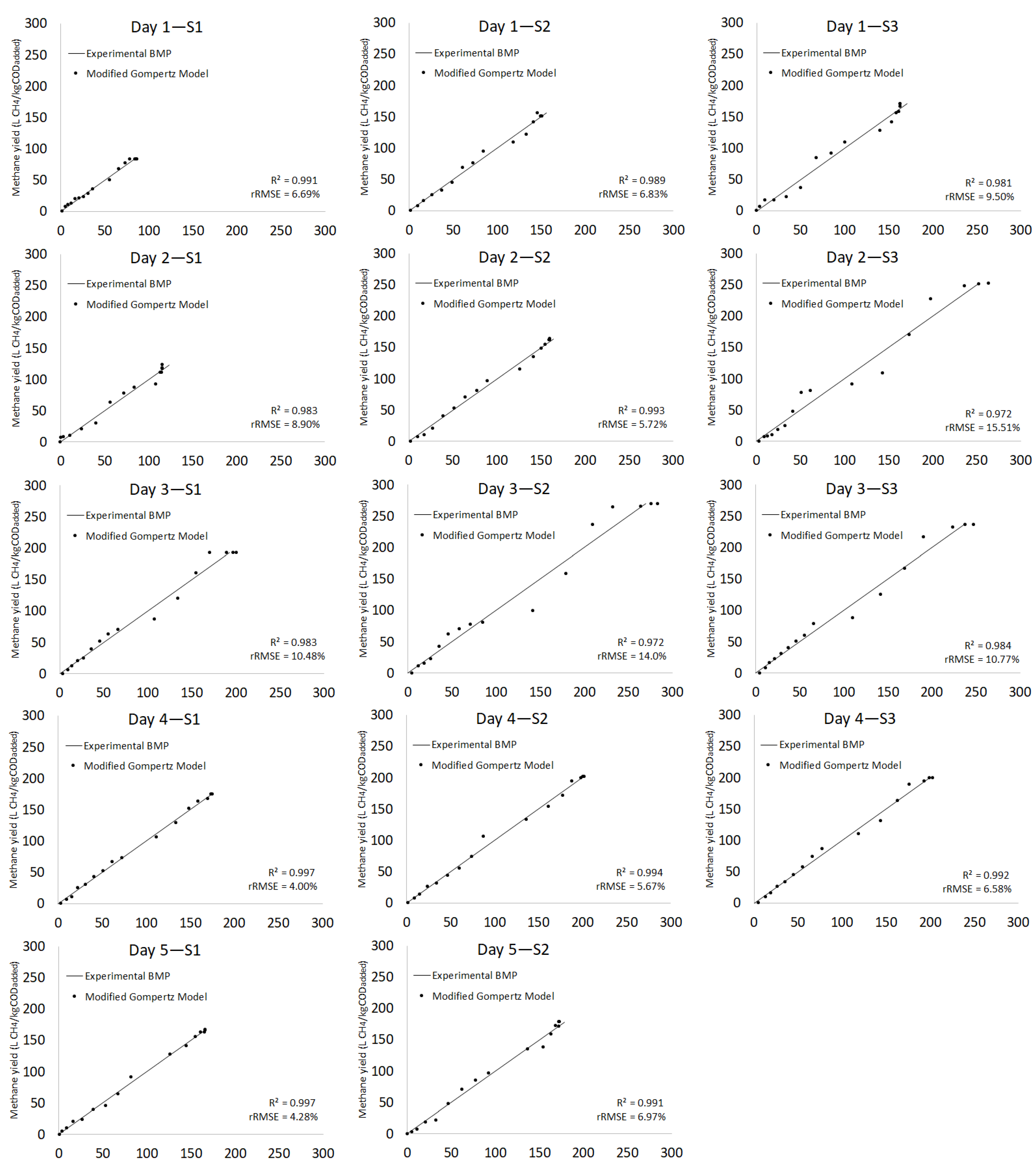
3.2.3. Kinetic Model

Figure 3 presents the comparison between the experiment and predicted methane yields. Table 3 summarises the estimated parameters for the studied first-order kinetic model and the modified Gompertz model. The kinetic parameters estimated include hydrolysis constant (Khyd), lag phase (λ) and Rmax during the anaerobic digestion of RWW. Among the two studied models, modified Gompertz model showed the lowest difference between the experimental and predicted methane yields (0 to 6.3%) than first-order model (0.8 to 18.7%). To evaluate the soundness of the model results, experimental methane yields were plotted against the predicted methane yields and presented in Figure 4. The statistical indicators (rRMSE and R2 values) were calculated and presented in Table 3. A lower rRMSE (4.0–15.51%) and higher R2 value (0.972–0.997) were obtained for the modified Gompertz model than for the first-order kinetic model (rRMSE = 3.97–17.55%, R2 = 0.956–0.994). Despite high R2 values, the modified Gompertz model did not provide a very accurate fit to the experimental data. Nevertheless, based on the kinetic study results (difference between predicted and measured methane yield, and statistically indicators) the modified Gompertz model was found to be a better model to fit the experimental methane yields. The possible reason for this observation is due to lag phase noticed for all samples in the study. A similar observation of a lag phase was reported during anaerobic digestion of apple waste with swine manure [42] and ensiled fish waste [43]. In both studies, the modified Gompertz model was shown as a better fit model to predict the methane yields compared to the first-order kinetic model. Both these results suggests that the methanogenic activity and methane production rates are highly dependent on the strength of RWW.
Table 3 presents the Rmax, time-delay (t), lag phase (λ) and khyd. There was no clear trend between the methane yields and the above kinetic parameters. The kinetic constants were calculated for 45 days of digestion time, but the time needed for 90% methane production (T90) fell within the range of 15.89–21.98 days. The variation in the kinetics of methane production could be due to presence of easily degradable substrate, slowly degradable substrate and, the amount and type of intermediate products generated during the anaerobic digestion. The hydrolysis constant (khyd), the constant rate at which the microbes digesting the available food would do so before they became inactivate, for the samples ranged from 0.09 to 0.21, with the highest value noticed for the S1—Day 2 (Table 3). The khyd values obtained in the present study are similar to those reported in the literature for livestock effluents [44]. On the other hand, a large time delay (3.84 d−1) was noticed for sample S3 of Day 2, which had the second-highest methane yields. The possible reason for this observation could be due to the accumulation of LCFAs during the hydrolysis of lipids, thereby inhibiting propionic acid’s degradation into smaller chain organic acids [38]. Several previous studies have shown that the rate-limiting step for RWWs was acidogenesis [11,38,39].
Table 3 also shows the effective methane production period (Tef). Tef was calculated by subtracting the lag time (k) from T90. Once again there was no clear trend in Tef values. Overall, Day 4 samples had the highest Tef values followed by Day 3 and Day 1 samples. One possible reason for the high Tef values in these samples could be due to rapid acidification and thereby inhibiting the methanogenic activity. This was evident by a lower Rmax values. A high Rmax values indicates that the rates of digestion are fast. Interestingly, S3 of Day 2 had high Tef (18.03 d) and low Rmax value (11.98 L CH4/kgCODadded/d) but resulted in producing relatively high methane yields of 252 L CH4/kgCODadded. Hydrolysis of rendering wastewater, rich in FOG and proteins, might have been the rate limiting step. Later, acidification of samples due to the formation of LCFA/VFA could have reduced ammonia inhibition and thereby further improved the methanogenic activity.
The results from the present study on the temporal variation in chemical composition of RWW suggests that a buffer tank should be installed at the full-scale biogas plant in order equalize the chemical composition and facilitate in uniform loading to biogas plant for stable anaerobic digestion process and methane yields. In addition, reduction in the amount of wash water and/or use of detergents can also reduce the variation in the daily wastewater characteristics.

4. Conclusions

The study showed that chemical composition of the incoming feed to a biogas plant varied throughout the sampled week and was dependent on the organic materials received and the amount of wash water used for washing the rendering process lines at the studied rendering plant. The results showed that COD, NH4-N, and VFA concentrations in the RWW varied significantly during the studied period (p ≤ 0.05) and had a profound influence on the methane yields (p ≤ 0.05). Depending upon the chemical composition and sampling time, methane yields of 83.7 to 270.2 L CH4/kgCODadded were obtained. Post digestion chemical analyses showed that methane yields, and COD removal rates were dependent on the readily biodegradable COD content in RWW. COD removal rates ranged from 61.69% to 80.79% with morning samples (S1) showing a slightly lower methane yields and COD removal rates than mid-day (S2) and evening (S3) samples. High methane yields and biodegradability from S2 or S3 samples was attributed to intensification of the rendering operations, type of raw materials received and their processing operations to value products and thereby generating high strength wastewaters. Thus, installation of a buffer tank to equalize the fluctuations in the chemical composition of wastewaters generated from the rendering plant could dampen the variation in the organic loading to the biogas plant and facilitate in steady biogas production.

Author Contributions

Conceptualization, E.C. and P.K.; methodology, E.C.; software, E.C.; validation, E.C. and P.K.; formal analysis, E.C. and P.K.; investigation, E.C.; resources, G.U; data curation, P.K.; writing—original draft preparation, E.C.; writing—review and editing, P.K.; supervision, P.K. All authors have read and agreed to the published version of the manuscript.

Funding

This research received no external funding.

Acknowledgments

Erika Conde PhD studies was supported by Griffith University Postgraduate Research Scholarship and Griffith University International Postgraduate Research Scholarship. The authors also greatly acknowledge rendering plant A J Bush & Sons, Beaudesert, Queensland for providing the research material.

Conflicts of Interest

The authors declare that they have no conflict of interest.

References

  1. OECD-FAO. OECD-FAO Agricultural Outlook 2022–2030; OECD Publishing: Paris, France, 2022. [Google Scholar]
  2. MLA. Industry Projections 2021—Australian Cattle; MLA: New York, NY, USA, 2021. [Google Scholar]
  3. NSW Environment Protection Authority. Future Use of Household Waste and Mixed Waste Organic Outputs; NSW Environment Protection Authority: Parramatta, Australia, 2019.
  4. AMPC; MLA. 2020 Environmental Performance Review (EPR) for the Red Meat Processing (RMP) Industry; MLA: New York, NY, USA, 2021. [Google Scholar]
  5. Xie, A.; Deaver, J.A.; Miller, E.; Popat, S.C. Effect of feed-to-inoculum ratio on anaerobic digestibility of high-fat content animal rendering wastewater. Biochem. Eng. J. 2021, 176, 108215. [Google Scholar] [CrossRef]
  6. Sindt, G. Environmental issues in the rendering industry. In Essential Rendering: All About The Animal By-Products Industry; Meeker, D.L., Ed.; The Animal Protein Producers Industry: Alexandria, VA, USA, 2006; pp. 245–272. [Google Scholar]
  7. Aziz, A.; Basheer, F.; Sengar, A.; Khan, S.U.; Farooqi, I.H. Biological wastewater treatment (anaerobic-aerobic) technologies for safe discharge of treated slaughterhouse and meat processing wastewater. Sci. Total Environ. 2019, 686, 681–708. [Google Scholar] [CrossRef] [PubMed]
  8. Laginestra, M.; van-Oorschot, R. Wastewater Treatment Pond Systems—An Australian Experience. In Proceedings of the Australian Water Association Conference, Melboure, Australia, 16–18 March 2009; 2009. [Google Scholar]
  9. Masse, L.; Masse, D. Effect of soluble organic, particulate organic, and hydraulic shock loads on anaerobic sequencing batch reactors treating slaughterhouse wastewater at 20 C. Process Biochem. 2005, 40, 1225–1232. [Google Scholar] [CrossRef]
  10. Shilton, A.; Harrison, J. Development of guidelines for improved hydraulic design of waste stabilisation ponds. Water Sci. Technol. 2003, 48, 173–180. [Google Scholar] [CrossRef]
  11. Harris, P.W.; McCabe, B.K. Review of pre-treatments used in anaerobic digestion and their potential application in high-fat cattle slaughterhouse wastewater. Appl. Energy 2015, 155, 560–575. [Google Scholar] [CrossRef]
  12. Harris, P.W.; McCabe, B.K. Process optimisation of anaerobic digestion treating high-strength wastewater in the Australian red meat processing industry. Appl. Sci. 2020, 10, 7947. [Google Scholar] [CrossRef]
  13. APMC. Wastewater Management in the Australian Red Meat Processing Industry; The Australian Meat Processor: Sydney, NSW, Australia, 2017. [Google Scholar]
  14. McCabe, B.K.; Harris, P.; Baillie, C.; Pittaway, P.; Yusaf, T. Assessing a new approach to covered anaerobic pond design in the treatment of abattoir wastewater. Aust. J. Multi-Discip. Eng. 2013, 10, 81–93. [Google Scholar] [CrossRef]
  15. McCabe, B.K.; Harris, P.; Antille, D.L.; Schmidt, T.; Lee, S.; Hill, A.; Baillie, C. Toward profitable and sustainable bioresource management in the Australian red meat processing industry: A critical review and illustrative case study. Crit. Rev. Environ. Sci. Technol. 2020, 50, 2415–2439. [Google Scholar] [CrossRef]
  16. Shende, A.D.; Pophali, G.R. Anaerobic treatment of slaughterhouse wastewater: A review. Environ. Sci. Pollut. Res. 2021, 28, 35–55. [Google Scholar] [CrossRef]
  17. Johns, M. Developments in Waste Treatment in the Meat Processing Industry: A Review of Literature 1979–1993; Meat Research Corporation: Sydney, NSW, Australia, 1993. [Google Scholar]
  18. White, T.; Johns, M.; Butler, B. Methane Recovery and Use at a Meat Processing Facility—King Island; Rural Industries Research and Development Corporation Australian Government: Barton, Australia, 2013.
  19. UNSW, C. Treatment of Abattoir Wastewater Using a Covered Anaerobic Lagoon; UNSW CRC for Waste Management & Pollution Control: Sydney, Australia, 1998. [Google Scholar]
  20. Filer, J.; Ding, H.H.; Chang, S. Biochemical Methane Potential (BMP) Assay Method for Anaerobic Digestion Research. Water 2019, 11, 921. [Google Scholar] [CrossRef]
  21. Holliger, C.; Alves, M.; Andrade, D.; Angelidaki, I.; Astals, S.; Baier, U.; Bougrier, C.; Buffière, P.; Carballa, M.; De Wilde, V.; et al. Towards a standardization of biomethane potential tests. Water Sci. Technol. 2016, 74, 2515–2522. [Google Scholar] [CrossRef] [PubMed]
  22. Angelidaki, I.; Alves, M.; Bolzonella, D.; Borzacconi, L.; Campos, J.L.; Guwy, A.J.; Kalyuzhnyi, S.; Jenicek, P.; Lier, J.B.V. Defining the biomethane potential (BMP) of solid organic wastes and energy crops: A proposed protocol for batch assays. Water Sci. Technol. 2009, 59, 927–934. [Google Scholar] [CrossRef] [PubMed] [Green Version]
  23. Pererva, Y.; Miller, C.D.; Sims, R.C. Existing empirical kinetic models in biochemical methane potential (BMP) testing, their selection and numerical solution. Water 2020, 12, 1831. [Google Scholar] [CrossRef]
  24. APHA. Standard Methods for the Examination of Water and Wastewater; American Public Health Association: Washington, DC, USA, 2005. [Google Scholar]
  25. Latif, M.; Mehta, C.; Batstone, D. Influence of low pH on continuous anaerobic digestion of waste activated sludge. Water Res. 2017, 113, 42–49. [Google Scholar] [CrossRef]
  26. Lachat, A.G. QuikChem® Method 10-107-06-2-A. Determination of Ammonia by Flow Injection Analysis. 2015. Available online: https://support.hach.com/ci/okcsFattach/get/1028334_4 (accessed on 1 June 2022).
  27. Sarojam, P. Analysis of Wastewater for Metals using ICP-OES. Perkin Elmer Instrum. 2010, 11. Available online: https://www.perkinelmer.com.cn/lab-solutions/resources/docs/APP_MetalsinWastewater.pdf (accessed on 1 June 2019).
  28. Beckett, N.M.; Cresswell, S.L.; Grice, D.I.; Carter, J.F. Isotopic profiling of seized benzylpiperazine and trifluoromethylphenylpiperazine tablets using δ13C and δ15N stable isotopes. Sci. Justice 2015, 55, 51–56. [Google Scholar] [CrossRef]
  29. Paulose, P.; Kaparaju, P. Anaerobic mono-digestion of sugarcane trash and bagasse with and without pretreatment. Ind. Crops Prod. 2021, 170, 113712. [Google Scholar] [CrossRef]
  30. Valero, D.; Montes, J.A.; Rico, J.L.; Rico, C. Influence of headspace pressure on methane production in Biochemical Methane Potential (BMP) tests. Waste Manag. 2016, 48, 193–198. [Google Scholar] [CrossRef] [Green Version]
  31. Astals, S.; Esteban-Gutiérrez, M.; Fernández-Arévalo, T.; Aymerich, E.; García-Heras, J.; Mata-Alvarez, J. Anaerobic digestion of seven different sewage sludges: A biodegradability and modelling study. Water Res. 2013, 47, 6033–6043. [Google Scholar] [CrossRef]
  32. Odirile, P.T.; Marumoloa, P.M.; Manali, A.; Gikas, P. Anaerobic Digestion for Biogas Production from Municipal Sewage Sludge: A Comparative Study between Fine Mesh Sieved Primary Sludge and Sedimented Primary Sludge. Water 2021, 13, 3532. [Google Scholar] [CrossRef]
  33. Auterská, P.; Novák, L. Successful solution for high nitrogen content wastewater treatment from rendering plants. Water Sci. Technol. 2006, 54, 23–30. [Google Scholar] [CrossRef] [PubMed]
  34. Brennan, B.; Gunes, B.; Jacobs, M.R.; Lawler, J.; Regan, F. Potential viable products identified from characterisation of agricultural slaughterhouse rendering wastewater. Water 2021, 13, 352. [Google Scholar] [CrossRef]
  35. Bustillo-Lecompte, C.F.; Mehrvar, M. Slaughterhouse wastewater characteristics, treatment, and management in the meat processing industry: A review on trends and advances. J. Environ. Manag. 2015, 161, 287–302. [Google Scholar] [CrossRef] [PubMed]
  36. Mousavi, S.A.; Khodadoost, F. Effects of detergents on natural ecosystems and wastewater treatment processes: A review. Environ. Sci. Pollut. Res. 2019, 26, 26439–26448. [Google Scholar] [CrossRef] [PubMed]
  37. Mensah, K.A.; Forster, C.F. An examination of the effects of detergents on anaerobic digestion. Bioresour. Technol. 2003, 90, 133–138. [Google Scholar] [CrossRef]
  38. Bayr, S.; Ojanperä, M.; Kaparaju, P.; Rintala, J. Long-term thermophilic mono-digestion of rendering wastes and co-digestion with potato pulp. Waste Manag. 2014, 34, 1853–1859. [Google Scholar] [CrossRef]
  39. Pitk, P.; Palatsi, J.; Kaparaju, P.; Fernández, B.; Vilu, R. Mesophilic co-digestion of dairy manure and lipid rich solid slaughterhouse wastes: Process efficiency, limitations and floating granules formation. Bioresour. Technol. 2014, 166, 168–177. [Google Scholar] [CrossRef]
  40. Bayr, S.; Rantanen, M.; Kaparaju, P.; Rintala, J. Mesophilic and thermophilic anaerobic co-digestion of rendering plant and slaughterhouse wastes. Bioresour. Technol. 2012, 104, 28–36. [Google Scholar] [CrossRef]
  41. Gutu, L.; Basitere, M.; Harding, T.; Ikumi, D.; Njoya, M.; Gaszynski, C. Multi-Integrated Systems for Treatment of Abattoir Wastewater: A Review. Water 2021, 13, 2462. [Google Scholar] [CrossRef]
  42. Kafle, G.K.; Kim, S.H. Anaerobic treatment of apple waste with swine manure for biogas production: Batch and continuous operation. Appl. Energy 2013, 103, 61–72. [Google Scholar] [CrossRef]
  43. Kafle, G.K.; Kim, S.H.; Sung, K.I. Ensiling of fish industry waste for biogas production: A lab scale evaluation of biochemical methane potential (BMP) and kinetics. Bioresour. Technol. 2013, 127, 326–336. [Google Scholar] [CrossRef] [PubMed]
  44. Garcia, N.H.; Mattioli, A.; Gil, A.; Frison, N.; Battista, F.; Bolzonella, D. Evaluation of the methane potential of different agricultural and food processing substrates for improved biogas production in rural areas. Renew. Sustain. Energy Rev. 2019, 112, 1–10. [Google Scholar] [CrossRef]
Figure 1. Effect of temporal variation in chemical composition on methane yields during the anaerobic digestion of rendering plant wastewater incubated in batch assays at 37 °C.
Energies 15 07252 g001
Figure 2. Methane yields obtained during anaerobic digestion of mean daily samples of rendering plant wastewater. Mean values per day in red line.
Energies 15 07252 g002
Figure 3. Comparison experimental and modelled data during the anaerobic digestion of rendering wastewater incubated in batch assays at 37 °C.
Energies 15 07252 g003
Figure 4. Experimental methane yields vs. predicted methane yields with Modified Gompertz model during the anaerobic digestion of rendering wastewater incubated in batch assays at 37 °C.
Energies 15 07252 g004
Table 1. Variation in chemical composition of rendering wastewater collected from Monday through Friday.
ParameterDay 1Day 2Day 3Day 4Day 5
S1S2S3S1S2S3S1S2S3S1S2S3S1S2
TS (%) a0.13 ± 0.00.28 ± 0.00.61 ± 0.10.44 ± 0.10.60 ± 0.11.82 ± 0.10.76 ± 0.10.66 ± 0.10.81 ± 0.21.02 ± 0.10.67 ± 0.10.75 ± 0.20.57 ± 0.00.54 ± 0.1
VS (%) a0.11 ± 0.00.21 ± 0.00.54 ± 0.10.34 ± 0.00.44 ± 0.11.44 ± 0.10.66 ± 0.10.56 ± 0.00.60 ± 0.20.72 ± 0.10.61 ± 0.10.67 ± 0.10.49 ± 0.10.45 ± 0.0
VS/TS0.800.740.880.780.730.790.860.860.740.710.910.900.870.83
COD (mg/L) a3747.0 ± 1.03966.5 ± 1.27586.6 ± 0.56873.3 ± 0.67605.3 ± 1.19047.9 ± 1.28153.3 ± 1.110,469.1 ± 1.09291.0 ± 0.97663.5 ± 0.98029.5 ± 1.18844.2 ± 0.97037.5 ± 1.06722.5 ± 0.8
NH4-N (mg/L) a52.2 ± 0.842.9 ± 0.945.4 ± 0.771.3 ± 0.963.3 ± 0.766.2 ± 0.361.2 ± 0.958.8 ± 0.858.2 ± 0.851.2 ± 0.265.9 ± 0.553.9 ± 0.759.9 ± 0.656.9 ± 0.6
PO4-P (mg/L) a52.2 ± 1.060.4 ± 1.233.1 ± 1.276.3 ± 2.160.2 ± 1.550.3 ± 1.763.2 ± 1.440.3 ± 1.533.5 ± 1.050.9 ± 0.960.2 ± 1.254.0 ± 1.051.4 ± 1.652.2 ± 2.3
TKP (mg/kg) a20.4 ± 2.525.7 ± 1.925.3 ± 2.220.4 ± 2.321.9 ± 2.020.6 ± 2.625.4 ± 2.231.0 ± 2.425.3 ± 2.130.4 ± 2.333.5 ± 2.421.7 ± 2.333.2 ± 2.232.2 ± 2.2
TKN (mg/kg) a112.7 ± 1.9265.7 ± 2.2151.0 ± 2.060.9 ± 2.170.6 ± 2.390.5 ± 2.5151.0 ± 2.360.9 ± 2.270.6 ± 2.140.5 ± 2.243.6 ± 2.298.6 ± 2.180.7 ± 2.198.7 ± 2.2
TVFA (mg/L) a149.1 ± 3.3189.5 ± 2.6288.8 ± 2.5177.8 ± 2.1198.1 ± 2.3267.5 ± 2.4217.6 ± 2.2384.7 ± 2.0455.4 ± 2.3212.7 ± 2.3227.0 ± 2.3280.8 ± 2.4241.4 ± 2.6247.7 ± 1.9
Acetic acid (mg/L)97.1111.7129.0103.7117.0212.3179.3217.4418.3163.5121.1146.2139.6243.8
Propionic acid (mg/L)30.577.694.950.160.128.630.4141.611.112.791.295.693.40.0
iso-Butyric acid (mg/L)12.80.013.26.90.816.20.03.48.812.20.24.61.13.9
Butyric acid (mg/L)0.00.015.710.011.97.20.09.48.112.36.512.61.80.0
iso-Valeric acid (mg/L)5.90.117.43.88.43.23.613.13.65.65.18.20.70.0
Valeric acid (mg/L)2.00.07.70.90.00.04.10.04.11.91.45.60.30.0
4-Methyl valeric acid (mg/L)0.90.05.51.20.00.00.10.00.10.81.83.90.20.0
Hexanoic acid (mg/L)0.00.05.01.10.00.00.00.01.23.70.04.24.50.0
Note: S—represent sample; a Average.
Table 2. Temporal variation in the chemical composition of the digestates obtained during the anaerobic digestion of rendering plant wastewaters in batch experiments at 37 °C.
ParameterDay 1Day 2Day 3Day 4Day 5
S1S2S3S1S2S3S1S2S3S1S2S3S1S2
COD (mg/L)1435.431203.752231.822560.522166.601966.832203.502011.572162.892317.652318.982544.032105.332011.04
% COD degradation61.6969.6570.5862.7571.5178.2672.9780.7976.7269.7671.1271.2470.0870.08
TKP (mg/kg)0.230.240.220.230.220.210.210.220.220.250.240.250.260.23
TKN (mg/kg)0.370.360.330.360.340.340.140.380.340.400.210.370.330.37
TVFA (mg/L)15.6616.1816.5217.1317.3118.3116.9818.7417.4318.1417.6117.5616.9917.98
Acetic acid (mg/L)10.4311.4711.8412.2712.4612.7211.9113.1612.5912.4512.2212.3011.7212.44
Propionic acid (mg/L)0.000.000.000.000.000.000.000.000.000.000.000.000.000.00
iso-Butyric acid (mg/L)0.000.000.000.000.000.000.000.000.000.000.000.000.000.00
Butyric acid (mg/L)1.781.871.721.841.811.911.871.831.691.931.961.681.721.88
iso-Valeric acid (mg/L)0.000.000.000.000.000.000.000.000.000.000.000.000.000.00
Valeric acid (mg/L)2.122.101.972.042.111.921.962.161.892.002.001.971.941.95
4-Methyl valeric acid (mg/L)0.330.730.990.990.941.381.240.971.271.761.431.611.301.70
Hexanoic acid (mg/L)0.000.000.000.000.000.380.000.620.000.000.000.000.000.00
Table 3. Kinetic parameters during the anaerobic digestion of rendering wastewater in batch experiment at 37 °C.
SampleExperimental Methane Yields
(L/kgCODadded)
First-Order Kinetic ModelGompertz Equation Model
Bo
(L/kgCODadded)
Difference (%)t (d−1)khyd (d−1)rRMSE (%)R2Bo
(L/kgCODadded)
Difference (%)λ (d)T90 (d)Tef (d)RMax
(L/kgCODadded d−1)
rRMSE (%)R2
Day 1S183.7 ± 1.3991.909.32.510.0912.070.97186.813.62.0618.5316.455.256.690.991
S2150.8 ± 1.41156.803.92.590.127.380.988150.720.12.0018.1516.1512.246.830.989
S3166.5 ± 1.39168.501.23.740.179.370.982163.002.13.1517.6714.5217.699.500.981
Day 2S1123.2 ± 1.71119.193.33.820.219.220.981115.686.33.6415.8912.2516.998.900.983
S2164.0 ± 1.70166.901.82.700.133.970.996160.132.42.0618.9216.8613.055.720.993
S3252.6 ± 1.73304.718.73.840.0517.440.964268.996.33.9521.9818.0311.9815.510.972
Day 3S1192.6 ± 1.27215.611.33.330.0813.530.972201.884.72.8520.1617.3110.7310.480.983
S2270.2 ± 1.25310.513.93.300.0717.550.956285.855.63.0919.7516.6614.3514.000.972
S3237.0 ± 1.00283.717.93.260.0614.730.970252.046.23.1421.7816.6411.2310.770.984
Day 4S1174.9 ± 1.17186.76.52.750.096.420.992175.450.32.3120.4918.1810.844.000.997
S2201.9 ± 1.16211.54.63.390.117.810.989201.930.02.6920.3217.6313.935.670.994
S3199.7 ± 1.10218.48.92.580.088.220.988203.511.92.0220.9318.9111.066.580.992
Day 5S1167.3 ± 2.82172.092.83.700.138.590.987166.090.73.3317.9914.6614.464.280.997
S2178.4 ± 280179.900.83.540.145.660.994172.753.22.9919.4716.4815.536.970.991
T90—Time taken for 90% methane production. Tef—Effective methane production duration (T90 − λ).
Publisher’s Note: MDPI stays neutral with regard to jurisdictional claims in published maps and institutional affiliations.

