A New Strategy for PI Tuning in Photovoltaic Irrigation Systems Based on Simulation of System Voltage Fluctuations Due to Passing Clouds

Abstract

One of the greatest challenges in stand-alone photovoltaic irrigation systems (PVIS) without batteries is the tuning of PID controllers and the evaluation of their performance once the system is tuned. Tuning method must be applied in clear days (constant irradiance) while performance must be evaluated in the most unfavourable circumstances, which occur when the passage of a cloud causes a sudden drop in available power. In short, tuning and testing must be done under different weather conditions. To solve this problem, a tuning method that is complemented by a method to simulate voltage fluctuations due to cloud passage has been developed. This allows tuning and evaluation of the system’s performance in the same session. Furthermore, the new PI tuning method achieves a better adjustment of the parameters and solves the instability problems that arise when applying traditional closed-loop tuning methods. Both methods use the feedforward input that most variable frequency drivers have. A signal generator is used to carry out the simulation of the clouds. This input is also used to introduce a triangular signal used for the tuning of the PI controller. The results show that the performance of the system, characterized by the voltage of the PV generator, with simulated clouds is similar to the response with real clouds. With regard to the tuning, the new method achieves better performance than previous methods. These methods can be applied on clear days, under conditions of constant irradiance, which greatly simplifies its implementation and greatly reduces the time required for commissioning the system.

1. Introduction

The technology of stand-alone high power photovoltaic irrigation systems (PVIS) without batteries is one of the most promising to reduce the serious impact on agriculture caused by the continuous increase in prices of electricity generated by conventional energy sources [1]. Traditionally, these systems have been implemented with batteries [2,3,4] or with grid support [5]. Not using batteries is only possible if the control system is robust to photovoltaic (PV) power variations.

A basic PVIS is made up of a PV generator, a variable frequency drive (VFD) and a centrifugal motor pump [6,7] that raises a variable water flow to a water pool. The water flow depends on the irradiance on the PV generator.

The VFD performs a proportional-integral-derivative (PID) control [8] that must keep the system operating stably on a prefixed supply voltage, that usually coincides with the maximum power point (control variable), by varying the frequency pump operation (output variable) [6].

The key to optimal PVIS performance is an adequate tuning of the control algorithm, a process that presents great challenges due to the non-linear and non-time-invariant nature of the system [9,10,11].

A comprehensive analysis of the classical tuning methods has been carried out in [12] and it was concluded that the best performing method was the AMIGO method.

In order to carry out the tuning process efficiently, high and stable level of irradiance (PV power) is needed, which corresponds to clear days without clouds.

Once the tuning has been carried out, a verification of the control parameters obtained for the system is needed. The tests have to be performed in the most demanding conditions, that is when there is a sharp drop of the available power supplied by the PV generator. It is usually due to the passage of clouds over it. As a result of this phenomenon there is a sudden drop in the voltage of the PV generator. If this voltage falls below the lower limit supported by the VFD, the system will immediately stop, triggering an alarm.

To carry out this test, it is necessary to wait for the appropriate weather conditions, which correspond to windy and sunny days “dotted” with black and compact clouds that produce sudden changes in irradiance clouds (cumulus type).

Due to the different climatic conditions necessary to perform the tuning and its evaluation, these processes must be carried out in different periods of time. Considering that it is often necessary to make adjustments to the tuning parameters to improve system performance, the definitive validation of a system can take a time interval of several months or even years [11].

This paper presents two new innovative methods. One method for tuning the PID control algorithm of PVIS and other method that allows the evaluation of the performance of a PVIS by simulating the effect on system voltage of the passage of clouds in the same climatic conditions as the tuning (clear days with constant irradiance).

On the one hand, the proposed new tuning method solves the most serious problems of the AMIGO method [8,12,13,14], previously used for tuning. This method subjected the system to an oscillation in order to find characteristic parameters of the system and thus find the tuning constants. With the new method, this is not necessary. It avoids subjecting the system to potentially dangerous oscillations. The new method makes use of the feedforward input (present in practically all VFDs with integrated PID control) to inject a triangular signal that produces a disturbance in the voltage of the PV generator.

In the course of this research, it was discovered that the system voltage, when a cloud passed, described a waveform very similar to the derivative of the available irradiance at the time of cloud passage. This behaviour, not surprisingly, carried over to the simulated cloud. It could then be stated that the voltage in a well-tuned system would describe the waveform equivalent to the derivative of the signal introduced by the feedforward input. Therefore, by introducing a known signal at the input, we expect the derivative of this signal in the voltage response of the system. This is what the new tuning method is based on.

On the other hand, the simulation of the effect of passing clouds on the system voltage allows to complete the entire control system configuration process in just one day, so that the PVIS can operate at full capacity from initial commissioning. The method consists of using again the feedforward input to inject a signal that produces a disturbance in the voltage of the PV generator equivalent to that caused by the passage of a cloud over the generator.

It is possible to find in the specialized literature a good number of papers on the influence of irradiance fluctuations caused by passing clouds on the power supplied by grid-connected photovoltaic plants. The initial studies were motivated by the disturbances that a high PV penetration could produce in relatively small isolated networks such as those that exist on islands [15,16,17,18]. These studies had the difficulty of requiring very high time resolution of irradiance and power data to analyse fluctuations [19,20]. Other studies focused on developing active procedures to mitigate PV power fluctuations using batteries [21,22,23] capacitors [24] or other alternatives [25]. Other works focused their efforts on passive mitigation, analysing the smoothing effect of the size of PV plants [26] or the effect of dispersing them in the territory [27,28] always with the aim of avoiding disturbances in the electrical system. Others focused on analysing irradiance fluctuations for short-term prediction of PV power [29,30]. However, to the best of our knowledge, this effect has not been studied in isolated systems without batteries such as PVIS where the irradiance fluctuation is translated into a disturbance in the DC system voltage.

To establish the relationship between the magnitudes of the system voltage drop, of the feedforward signal and of the cloud that it simulates, a characterization work of the most frequent clouds has been carried out. To do this, the PVIS system has been running for several months and all relevant variables have been recorded. Afterwards, two of the most representative clouds have been chosen to experimentally verify the validity of the simulation method.

It has been found that the response of the PV generator voltage to the decrease in irradiance of a real cloud is similar to that which occurs on a clear day when a signal proportional to the inverted irradiance curve is applied to the feedforward input. The difference that can be found is in the amplitude of the voltage signal obtained. A larger amplitude in the input signal means a larger voltage drop, but it always keeps the same waveform. At the same input amplitude, the behaviour also changes depending on the tuning parameters. A better tuned system also produces a smaller voltage drop, but also retains the original waveform.

2. Materials and Methods

This section illustrates the research design including the infrastructure needed for the research (specific laboratory for experimentation with PVIS) and the methodology for both, the simulation of system voltage drops caused by passing clouds and the new PID tuning for PVIS.

The methodology for the simulation of system voltage drops caused by passing clouds has the following main steps:

• Data collection of the PVIS system operation under different passing clouds.
• Data analysis to identify clouds.
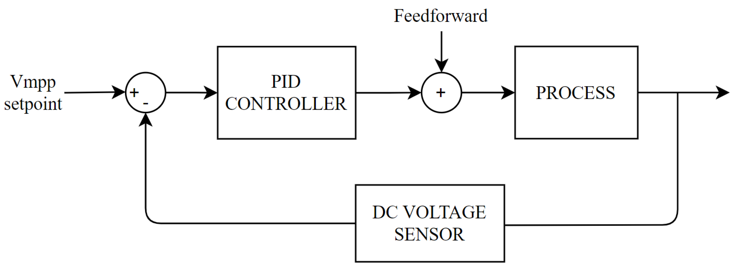
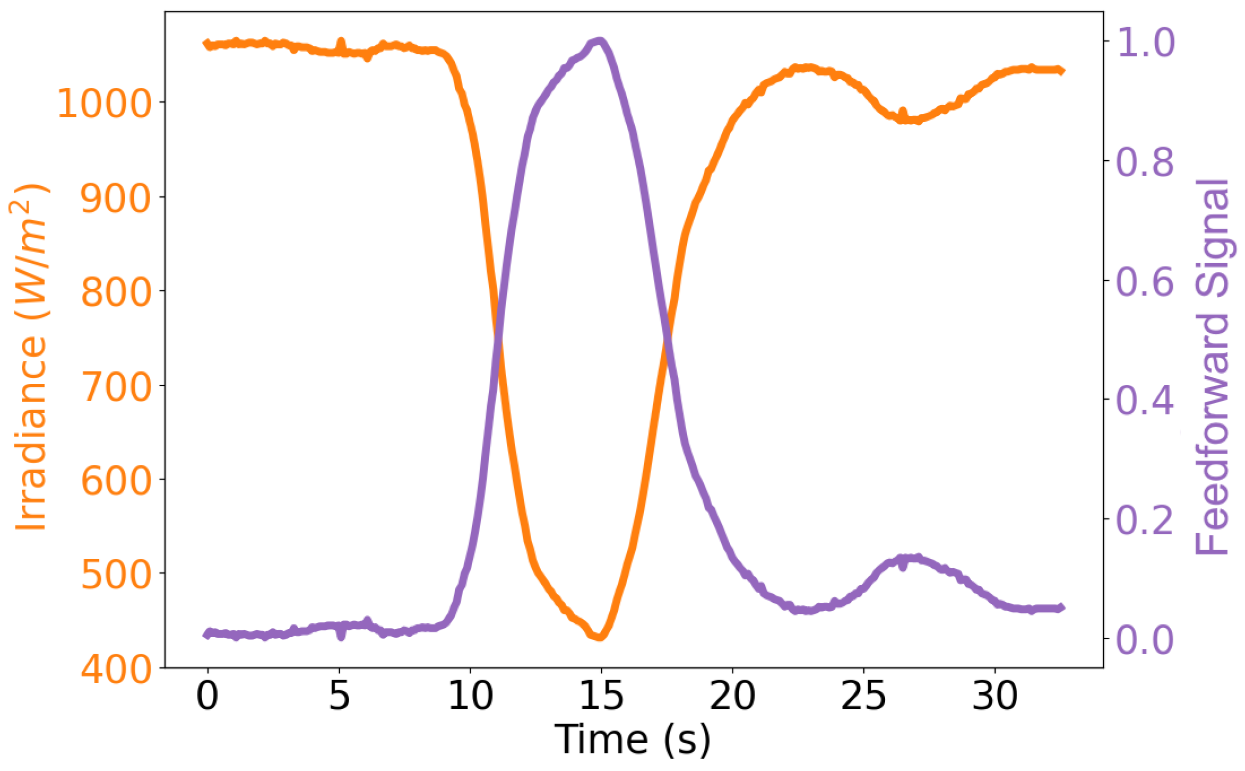
• Method for simulation using the feedforward input.

The methodology for the research of the new PID tuning method has the following steps:

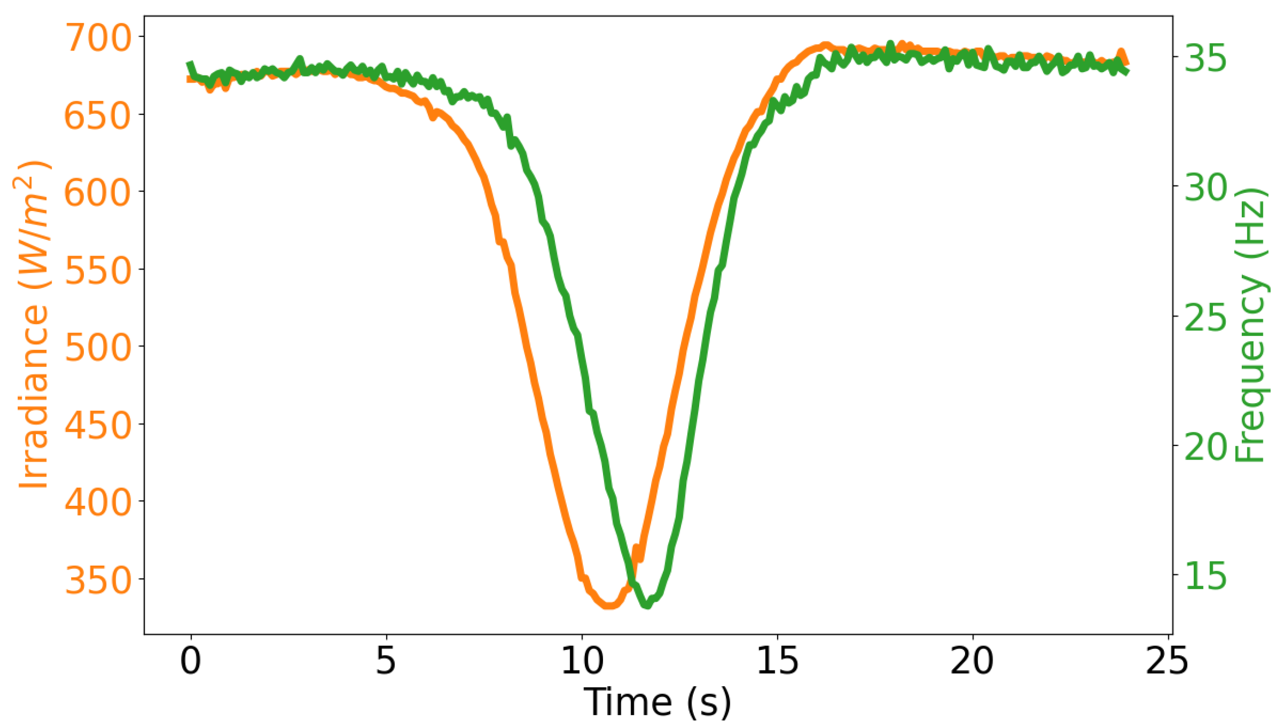
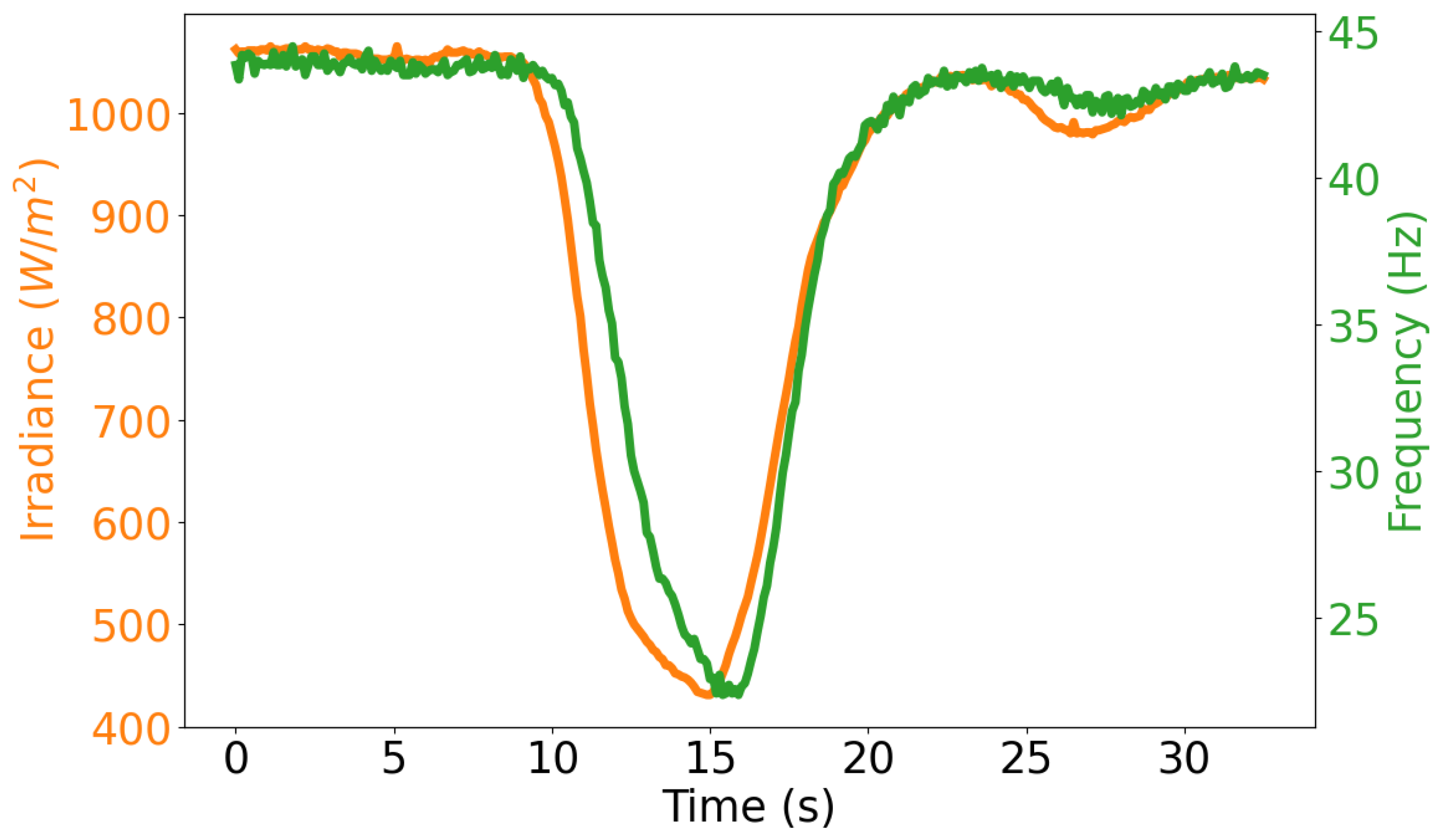
• The definition of the most suitable feedforward signal for the PID tuning based on the relationship between the system voltage, the derivative of irradiance and the output frequency.
• Development of the tuning process for both, stable operation and start-up of the PVIS. This section has been structured accordingly.

2.1. Laboratory Experimentation System

The laboratory where tests have been performed is made up of:

• PV array. $P=170$$W_p$; $V_{mp}=277.1$V.
• Variable frequency drive (VFD). Three-phase 200 V; 0.75 kW.
• Centrifugal fan connected to an induction motor to simulate a hydraulic pump [31,32,33,34].
• A monitoring and control system using:

  -

  Arduino based PLC (IndustrialShields).

  -

  MQTT for communication protocol.

  -

  Voltage, current, irradiance and temperature sensor. Frequency can be obtained from VFD.

• Oscilloscope and signal generator.

The PV array consists of 4 independent strings with 17 PV modules of 36 cells in series. Modules in each string are also connected in series. Arrays are connected in parallel, but it is possible to connect or disconnect them independently. This is useful to test the system with different available power. PV arrays are oriented to the south with a tilt angle of 45°. More detailed information on the system can be found at [12].

The irradiance, solar cell temperature and ambient temperature is provided by a calibrated PV cell with the same orientation.

The PV voltage array is measured by a voltage sensor with 0–1000 VDC input connected to the PV array and 0–10 VDC and 4–20 mA output. It is connected to the VFD as feedback signal of the PID control algorithm and to the monitoring system.

The hydraulic pump is simulated with a centrifugal fan driven by a 275 W standard induction motor in an air closed circuit, simulating water flow. The VFD to control the induction motor is OMRON 3G3RX-A2004 model.

The monitoring system, which uses MQTT protocol for communication, saves all the data in a csv file in the server. It has a sample time of 100 ms. This allows the visualization of the data in real-time and the subsequent analysis.

The oscilloscope and signal generator is a Digilent Analog Discovery 2. It is used to visualize the voltage curve and to generate any kind of signal (maximum amplitude in signal generator is 5 V due to USB power supply), which is necessary to simulate clouds.

2.2. Methodology to Simulate System Voltage Drops Caused by Passing Clouds

-

Step 1: Data collection

The first step is to store as many data as possible in days with different types of clouds. Changes in irradiance need to occur in order to produce disturbances in the system voltage. Because of that, extremely cloudy days are not good for this purpose.

As we can control the VFD remotely, it is possible to store data only if a day is interesting. It also can be programmed to run automatically when PV system provides enough power.

-

Step 2: Data analysis to identify clouds

A 100 ms sample time is enough to get irradiance and voltage disturbances produced by passing clouds. Smaller sample times are possible, but not needed for this application.

To analyse the data, several python programs have been developed. These programs are based on libraries for data analysis and filtering such as matplotlib, pandas or numpy. The program also has a graphic user interface.

This software analyses the collected data calculating the derivative of the irradiance curve. This derivative is the input of an algorithm to identify the clouds. It works as follows:

• Cloud recognition starts when the value of the calculated derivative is below the set threshold.
• Each of the derivative samples is analysed until its value is close to 0. If irradiance is stable, the cloud has finished.
• Advanced cloud filtering is available. For example, it can be configured to only display clouds that cause an irradiance decrease of a given value or given duration.

Figure 1 shows some of the clouds detected with the algorithm, being represented the irradiance and its derivative. Clouds detected are marked in colours automatically. Colours are random and only serve to differentiate between clouds.

-

Step 3: Simulation of system voltage drop caused by clouds using the VFD feedforward input

Clouds can be defined as a sudden decrease in irradiance and, consequently, a decrease in available PV power. Disturbances in DC voltage are produced because the PID response is not fast enough to react to the sudden power decreases.

The more aggressive a cloud is, the more voltage drop produces. The aggressiveness of the cloud depends on how fast the irradiance comes down and, as shown in Figure 1, it can be analysed using the derivative of irradiance curve. The DC voltage decreases in a greater proportion when the slope of the derivative of the irradiance is bigger (more aggressive).

For the following analysis, two clouds have been chosen and not just one, in order to demonstrate that the simulation process works correctly with different cloud shapes. Both are similar in duration and in irradiance drop (Cloud 1: 50.59% and Cloud 2: 59.41%). Main difference is the shape and the starting point of the irradiance.

These clouds come from days with cumulus type clouds and strong wind. The fastest and darkest clouds have been selected, as they produce the highest irradiance drop in the shortest time. By choosing this type of clouds, the system is being tested under the most unfavourable conditions possible (very abrupt fluctuations in the available PV power).

Figure 2 and Figure 3 show the irradiance and voltage signal when two different cloud passages occur.

The voltage perturbations that they produce are different, in both shape and amplitude, for each cloud. Different real clouds produce a different voltage drop and waveform, which will depend on the waveform that the irradiance describes due to the passage of the cloud. So, the temporal pattern of voltage disturbance caused by passing clouds does not remain unchanged but it depends on the irradiance waveform caused by a passing cloud. So each passing cloud produces a different temporal pattern of the system voltage drop.

These voltage disturbances affect the PVIS control. A PID controller is in charge of maintaining the PV generator voltage working in its maximum power point. The controller continuously adjusts the output operation frequency of the motor to keep the system working in the fixed voltage, that is the maximum power point voltage. For this, a sensor is constantly monitoring the actual system voltage, which will be the feedback to the PID controller.

Most VFD on the market are equipped with an input called feedforward. It is an external frequency input. When a signal is applied to this input, a frequency equivalent to the magnitude of this signal is added to the output frequency.

A diagram of how this input works is shown in Figure 4.

The proposed method uses this signal to simulate the system voltage disturbances caused by clouds. If a frequency is added to the output frequency, the power demanded by the motor to the PV generator will increase. This will cause a sudden decrease in DC voltage which the PID controller will correct decreasing the output frequency to maintain the fixed voltage. That is exactly the same behaviour as when a real cloud is passing and available PV power drops suddenly.

To have a good system voltage drop simulation using the feedforward input, it is very important to have a constant irradiance conditions, the same one needed to carry out the tuning process. This is a great advantage because two actions (system voltage drop simulation and tuning) can be performed in the same session.

In order to simulate a change in irradiance and its corresponding voltage drop through a frequency input, it is necessary to analyse how the frequency of the system behaves when the cloud passes over the PV generator.

As Figure 5 and Figure 6 show, frequency response and irradiance describe similar curves. This occurs because of the operation of the PID. When a cloud passes and there is a drop in irradiance, the controller reacts by lowering the frequency so that the voltage remains stable.

This opens the door to use irradiance as signal to simulate clouds and their effect on system voltage. So, the feedforward input to simulate the system voltage drop is built as follows:

• Get maximum value of the irradiance curve corresponding to a passing cloud.
• Subtract each irradiance sample to the maximum obtained in the first step.
• Divide by the maximum of the curve to normalize and get 1 as maximum.

The shape of the curve obtained is the same that the inverted irradiance because it has to be added through the feedforward input as a positive signal. The minimum point in the irradiance is now a maximum in the feedforward signal with an amplitude of 1. This means that we get a signal that has the same waveform as the original, but the level of disturbance it produces will depend, as we will see later, on the total amplitude of the signal.

To change the amplitude of the feedforward signal, it is necessary to multiply it by a constant. This way, the amplitude of the feedforward signal will be proportional to the disturbance it produces on the system voltage (see Section 3.1 for more details).

The feedforward signal to simulate the system voltage drop corresponding to Cloud 2 is shown in Figure 7.

2.3. PID Tuning Method

For the new tuning method, the feedforward input will also be used.

2.3.1. Most Suitable Feedforward Signal for PID Tuning Based on the Relationship between System Voltage, Derivative of Irradiance and Output Frequency

In all recorded clouds it has been observed that there is a direct relationship between the irradiance derivative and the system voltage. An example is shown in Figure 8.

In the previous section it was shown that it is possible to simulate the behaviour of the system voltage in the presence of a cloud by applying a signal equivalent to the irradiance at the feedforward input. Based on this, we hypothesise that the response of system voltage should be very similar to the derivative of the signal applied to the feedforward input.

This assumption is based on the operation of the PVIS controller. The frequency output of the controller is given by the PID operating Equation (1). Note that we have eliminated the derivative component of the PID because, in this type of systems, where electromagnetic noise is high, the value of the derivative constant is zero as it would cause instabilities and undesirable oscillations. This is the reason why, from now on, we will denominate the control as “PI” instead of “PID”.

$$f=K_p·(V-V_{sp})+K_i\int (V-V_{sp})\mathrm{d}t$$

(1)

where:

f = frequency output of VFD.

$K_p$ = proportional constant of PI controller. V = instant voltage of the PV generator.

$V_{sp}$ = setpoint of PI controller (mppt voltage).

$K_i$ = integral constant of PI controller.

In stationary operation, i.e., when the system is operating without any disturbances and is well tuned, the set-point voltage will be equal to the actual system voltage, so that the proportional part can be omitted at a given instant.

Then, we obtain Equation (2).

$$f\approx K_i\int (V-V_{sp})\mathrm{d}t$$

(2)

If we isolate the voltage from this equation, we obtain what can be seen in Equation (3), that is a linear relationship between the control variable (system voltage) and the derivative of the output variable (frequency applied to the motor).

$$V=V_{sp}+{\displaystyle \frac{1}{K_i}}{\displaystyle \frac{\mathrm{d}f}{\mathrm{d}t}}$$

(3)

So, in the same way that the system voltage signal follows the same shape as the derivative of the irradiance due to PI tuning, the system voltage signal follows the shape of the derivative of the inverted feedforward input as well.

Based on this, it has been hypothesised that the most suitable type of signal for PI tuning is a triangular signal.

The derivative of a triangular signal is a square signal. This type of signal makes it possible to visually and clearly identify the voltage drop on the DC bus, which will allow testing sets of tuning parameters efficiently and without the need for calculations.

Therefore, good tuning should respond with a square signal in voltage when a triangular signal is applied through the feedforward input.

2.3.2. Tuning Process

The first prerequisite for the tuning process is a PVIS system that operates stably. This means that the day must be sunny to avoid external disturbances.

An initial tuning must ensure that the system remains working stably, without oscillations. As there will be no external disturbances in the tuning process because clear days were selected, it is possible to find a wide combination of PI parameters for initial tuning that make the system stable.

It is important to note that at the time of tuning, the available irradiance and, consequently, the power, do not cause the PID to saturate under any circumstances. This would occur if the system reaches its maximum frequency with the available PV power, 50 Hz in this case.

Ideal frequency values at the time of initial tuning would be between 40 and 45 Hz.

Experience with such PVIS systems has shown that optimal values for $K_p$ are around a few units and for $T_i$ around tenths of a second. It has been found [11] that as PVIS nominal power increases, $K_p$ tends to be lower and $T_i$ similar.

Therefore, good initial parameters for tuning should meet the following requirements:

• $K_p$ smaller than optimal.
• $T_i$ larger than optimal.

For example, for the 170 $W_p$ system tested, after tuning with new method, optimal constants values would be $K_p=3$ and $T_i=0.03$. Consequently, correct values to start tuning could be $K_p=2$ and $T_i=0.1$.

By using parameters that comply with the above, the PI controller will react slowly to changes, ensuring stability. As there will be no disturbances, a very stable system will be achieved.

A triangular signal with a 5 s period has been set to perform the tuning process. This value is used because it is close to the time it takes for the irradiance to fall in the clouds analysed, although tests show that this time can be variable. What will be modified in this tuning process is the amplitude. The amplitude of the signal is directly proportional to the disturbance it produces in the system voltage. This would mean that, for large amplitudes, the system must be well tuned to bear the system voltage disturbance.

In order to avoid possible system failures, such as dangerous voltage drops, very small amplitudes are used as a starting point. The amplitude will increase as the tuning parameters are progressively modified and the system reacts to the changes. It should be borne in mind that the proposed method is iterative, so it will be necessary to spend time repeating the various tests and modifying the parameters according to the behaviour.

As mentioned above, the controller used is a PI. The parameters to be modified are $K_p$ and $T_i$. According to the tests carried out, each of these parameters affects the tuning in a different way (see Section 3.2.1).

In summary, the change of parameters affects the system in the following way:

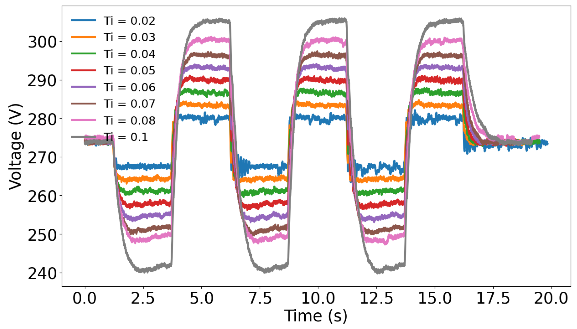
• $K_p$ modifies the system voltage waveform. The larger $K_p$ is, the smoother the step of the squared signal of the system voltage. If it is too small, oscillation occurs, which can be dangerous for the PVIS. This is true when using small $T_i$, which is what happens in this type of system.
• $T_i$ modifies the total amplitude of the system voltage signal. Low $T_i$ values result in low amplitudes, but making it too small results in an unstable and oscillating system.

From this initial point, the following tuning method is proposed:

• A triangular feedforward signal with a certain amplitude is chosen. At the beginning it should be very small but enough to produce a noticeable disturbance. It is important to note that it is not sufficient to introduce only a single disturbance. A train of at least two pulses of the triangular signal shall be introduced.A train of changes in the slope of the signal will produce more noticeable disturbances that would not occur with a single pulse.
• The value of $K_p$ is progressively increased and the triangular pulse train is reintroduced until the voltage response is as close as possible to a square wave. If a waveform as close to a square wave as possible is not achieved, the value of $T_i$ should be slightly reduced. See details in Section 3.2.1.
• The $T_i$ is gradually lowered until a small amplitude is reached in the train of square pulses of the system voltage, but without causing the system to oscillate and become unstable.
• The amplitude of the triangular signal is slightly increased so that the disturbance in the system voltage is greater. Repeat steps 2 and 3 again adjusting the parameters until the triangular signal amplitude is close to the maximum of the input feedforward (50 Hz) and is supported by the system.

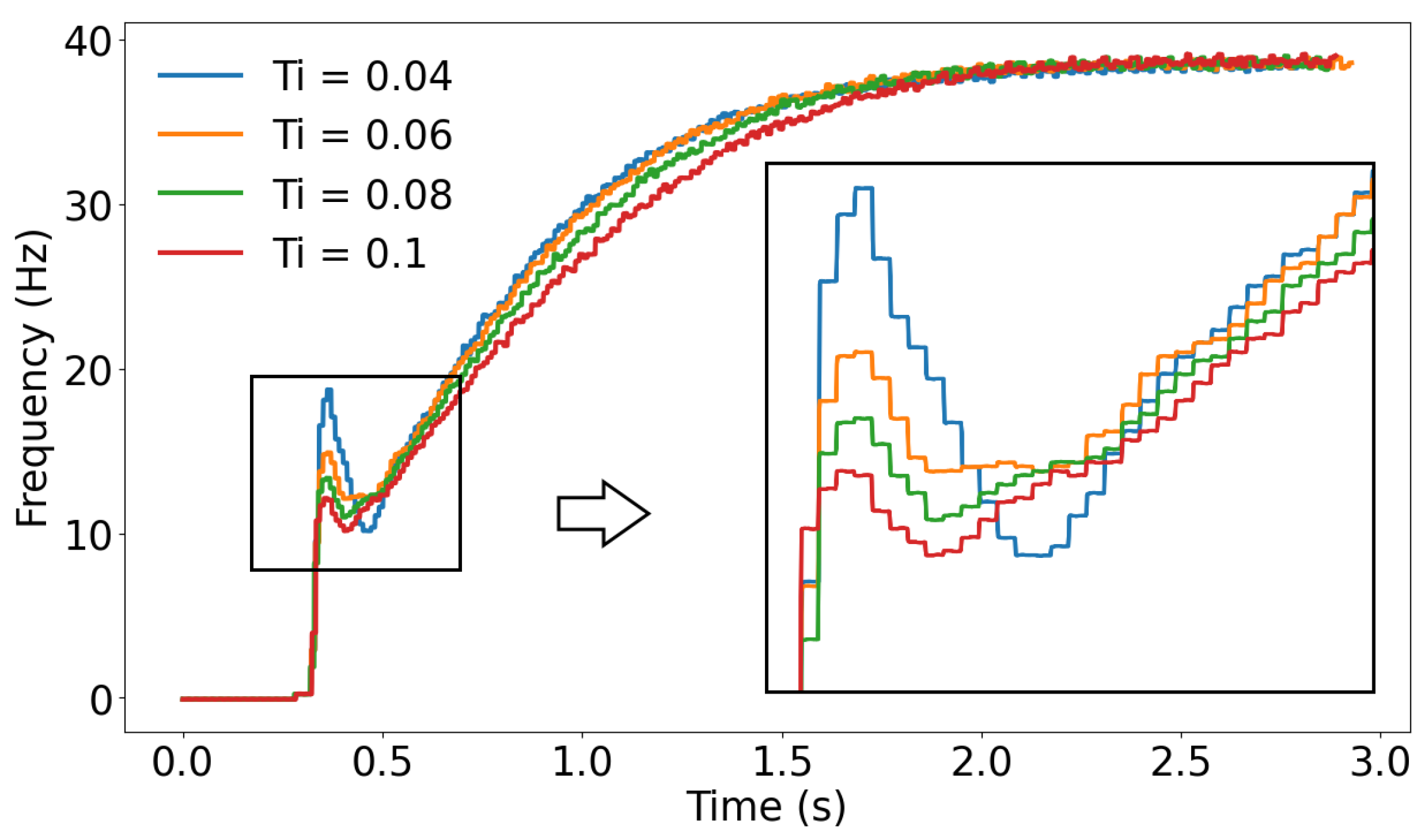
2.3.3. Tuning for Start-Up

It is important to remember that the system to be controlled is not linear. This method provides PI parameters that are valid when the system is already started and running. The problem arises precisely when the system starts from a standstill. These parameters would not work correctly.

At this point, there are two options:

• Program an adaptive PI. This means that the PI parameters at start-up and in normal operation will be different.
• Compromise to obtain an acceptable start and behaviour in all situations.

The preferred option, whenever possible, is the first option. This will ensure greater resistance to cloud passage and better overall performance.

With the different tests that have been done in the laboratory, it has been seen that, having tuned the system with the proposed method, good start-up PI parameters would follow the following rule: $K_p$ is lowered and $T_i$ is raised in the same proportion. For the system where test have been carried out, after tuning, good start-up parameters would be:

• $K_p/3$
• $T_i·3$

If it is not possible to have different parameters for the start-up and for the normal operation, it will be necessary to modify the parameters obtained in the proposed tuning method to start correctly. It could be used the above rule, but it will not be possible to make such large modifications without sacrificing correct operation once the system has started. A compromise must be found. In Section 3.2.2, different start-up behaviours that help to understand the above, are shown.

3. Results

Several tests have been performed to determine the relation between DC voltage and simulated clouds. The results of these tests have shown that there is a direct relationship between the amplitude of the feedforward signal and the voltage drop of the system.

The same feedforward input was used to carry out the tuning process using a triangular signal. Many combinations of PI parameters have been tested to show the system response (voltage and frequency operation) when using the new tuning method.

Finally, a simulation of a cloud comparing different sets of PI parameters is carried out to demonstrate how well the new tuning method works.

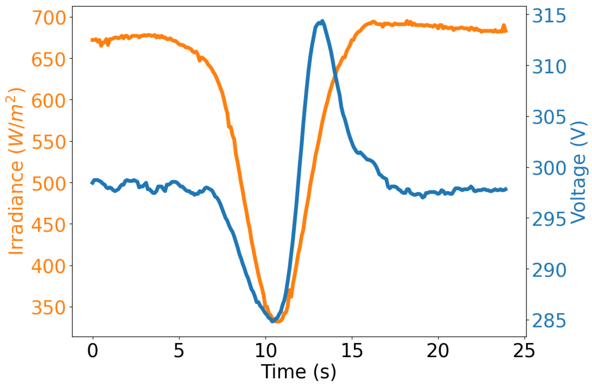
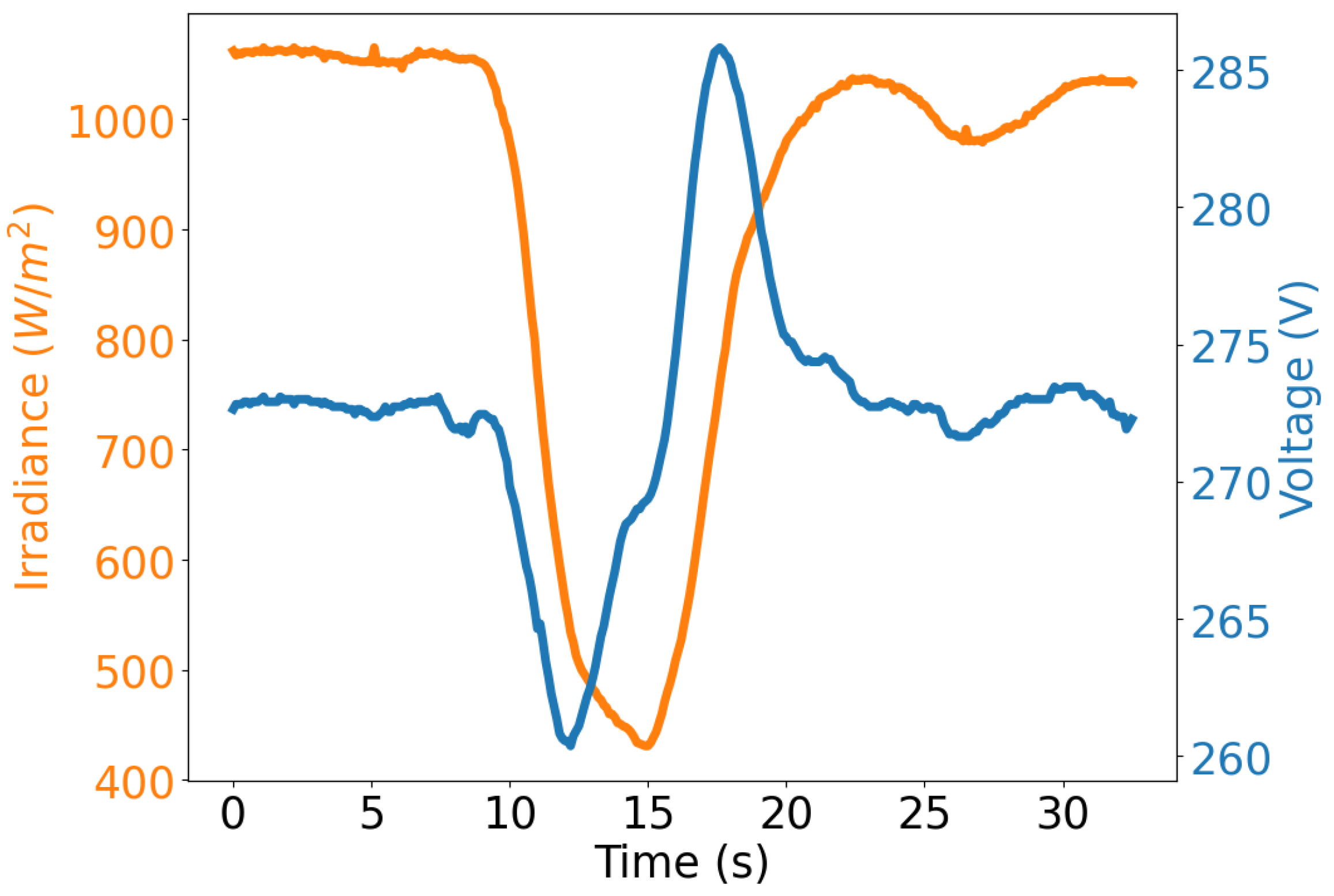
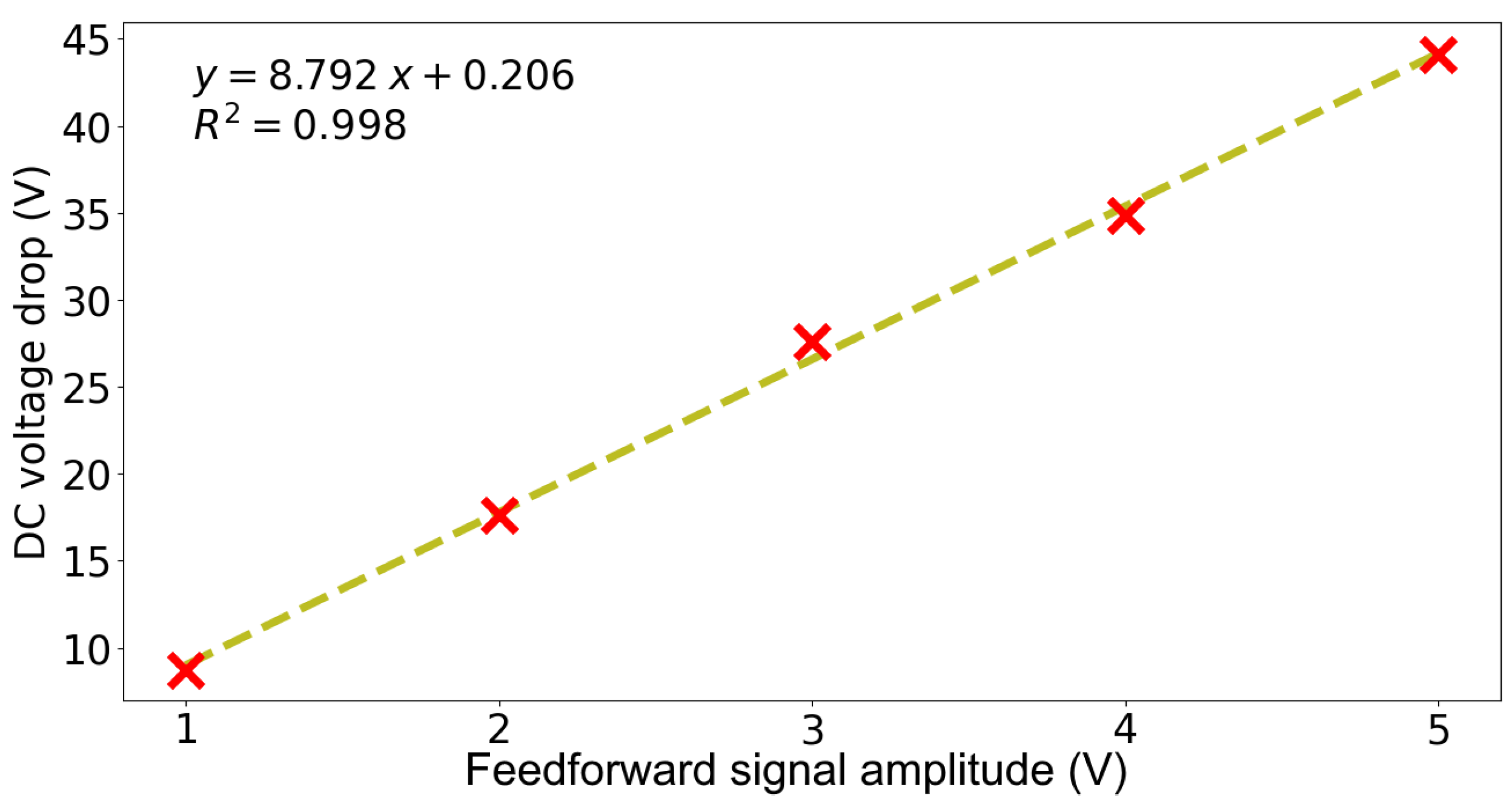
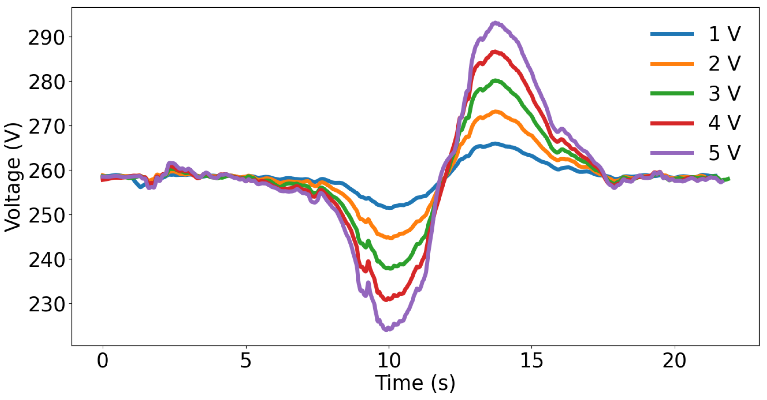
3.1. Results Related with the Simulation of System Voltage Drop Caused by Passing Clouds

One of the main objectives pursued by this work is to achieve the same DC voltage drop in the PVIS system with a simulated cloud using the feedforward input as with a real cloud. Initial feedforward signals are normalized but their amplitudes have to be scaled up (multiplying the normalized signal by a constant) to reproduce the system voltage drop for cloud 1 (Figure 2) and cloud 2 (Figure 3).

Table 1. DC voltage drop with different cloud signal amplitudes.

	DC Voltage Drop (V)
Feedforward Amplitude (V)	Cloud 1	Cloud 2
1	7.19	8.73
2	14.14	17.63
3	20.84	27.63
4	27.05	34.82
5	34.56	44.1

shows the results of the different system voltage drops for different feedforward signal amplitudes.

This behaviour is due to the action of the PI controller and the operation of the feedforward input previously explained. When the generated signal is added to the frequency output of the PI, the PI reacts to this change. The higher the amplitude of the feedforward signal, the more correction the PID must make, lowering its output. For this reason, the voltage drop depends on the amplitude of the feedforward signal used.

Figure 9 and Figure 10 show that, in addition, the relationship between amplitude of the feedforward signal and the voltage drop is linear. The slope of the straight line depends on the conditions under which the test has been carried out, mainly on the cell temperature of the PV generator. Once the equation of the line has been obtained, the value of the voltage signal amplitude that should be used for the feedforward input to obtain a particular voltage drop value can be calculated.

Furthermore, as shown in Figure 11 and Figure 12, the change in the amplitude of the feedforward signal does not affect to the voltage drop shape, that remains unchanged for a specific cloud. This means that the voltage drop caused by a specific irradiance disturbance caused by a specific cloud can be achieved using in the feedforward input the normalized inverted signal of the irradiance (to reproduce the shape) and modifying its amplitude accordingly to reproduce the amplitude of the voltage drop.

Figure 13 and Figure 14 show the system voltage response for clouds 1 and 2, with real and simulated clouds, to compare their shapes. It can be seen that the shapes of both curves are similar. The voltage scale is not the same because the samples of real and simulated clouds have been collected at different maximum power point voltages. This is because the real cloud sample was taken in winter, when the working voltage is higher due to lower temperatures. The simulation was performed in months where the temperature was higher, so the maximum power point voltage was smaller.

This demonstrates that the effect on system voltage of a real cloud can be simulated very accurately by applying the appropriate signal to the feedforward input under constant irradiance conditions.

3.2. Results Related with the New PI Tuning Method

3.2.1. Tuning for Normal Operation

To see how the use of the triangular signal through the feedforward input affects the system voltage, different tests have been made for different values of $K_p$, maintaining a value of $T_i$ and vice versa.

Figure 15 shows the system voltage when the triangular feedforward signal is introduced for different values of $K_p$ and $T_i=0.1$.

As said before, a good value of $K_p$ is one that makes the voltage signal as close to a square signal as possible (derivative of the triangular feedforward signal). As can be seen in Figure 15, this value is between 2 and 3. For smaller values, an overshoot in the system voltage signal is observed, while for larger values, the response slope is smoother.

In Figure 16, the $T_i$ is doubled. As can be seen, there is a smoothing of the curves, but the voltage value drops more sharply (observe that the voltage scale is different than Figure 15), because the system also becomes slower with increasing $T_i$. This is not what is needed in PVIS systems and, therefore, the parameter $T_i$ should have always small values for the system voltage disturbance to resemble the square signal and to have faster responses.

Once a suitable value of $K_p$ is obtained, different values of $T_i$ are tried. This can be seen in Figure 17, where the signal keeps the same shape, but the amplitude changes. Extreme values would not be good because the system would not be robust. In the other hand, with values very close to 0, small oscillations start to occur, which would increase the risk of instabilities. However, lower values reduce the system voltage drop, so a correct value would be around Ti = 0.03.

3.2.2. Tuning for Start-Up

Figure 18, Figure 19 and Figure 20 show the system voltage at starting phase for $K_p=1$, $K_p=2$ and $K_p=3$ with different values of $T_i$.

It can be seen that, if the value of $k_p$ increases, the system is more unstable and may oscillate at the starting phase. This is a very undesirable behaviour.

Higher values of $T_i$ with smaller values of $K_p$ produce a softer start-up, greatly reducing the peak voltage drop. However, voltage is not the only variable to consider, system frequency must also be considered. In Figure 21, Figure 22 and Figure 23 same tests are shown, but now, showing the system frequency at the start-up.

Controlling the system voltage drop is very important, but a small oscillation at start-up is not critical. At start-up, it is more important to control oscillations in system frequency, as the pump’s health could be affected by sudden changes in this variable.

The ideal start-up will be one in which the frequency describes a fast (about 2 s) and monotonically increasing rising curve. However, it is not possible to obtain good start-up and normal operating values at the same time. The solution, as already mentioned, is to find a compromise between the ideal parameters for start-up and normal operation. A good value, used only for start-up, would be $K_p=1$ and $T_i=0.1$, as shown in Figure 21. However, as seen in Figure 17, an optimal value for normal operation and to support the cloud pass would be $K_p=3$ and $T_i=0.03$.

Due to the programming restrictions of some inverters, not all possible parameter combinations are programmable. In this case, to reach the compromise, a good value that meets both conditions is $K_p=2$ and $T_i=0.1$.

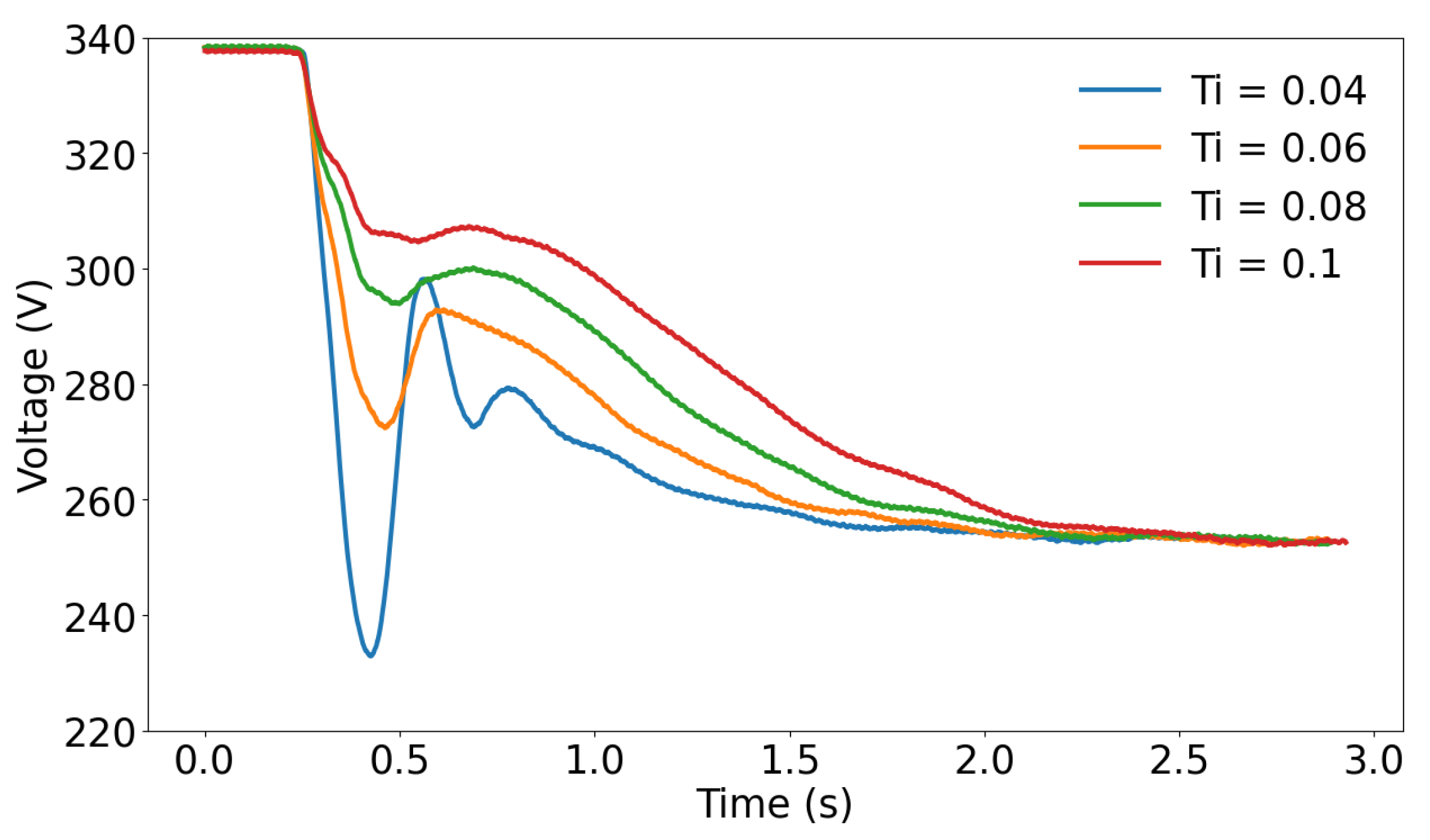
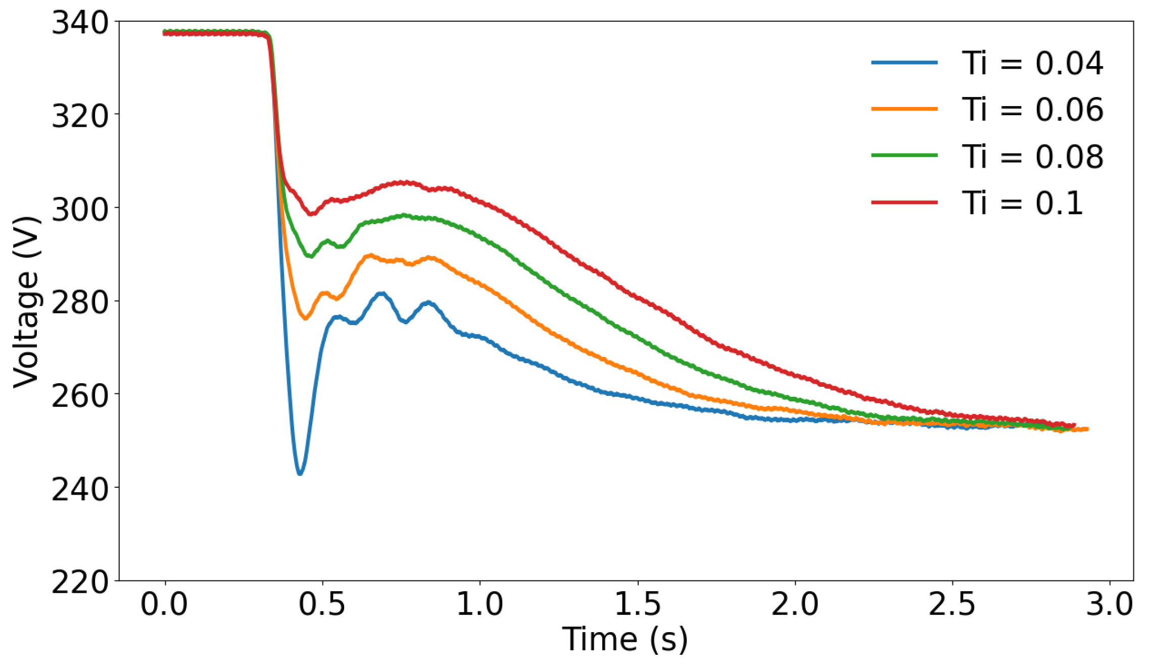
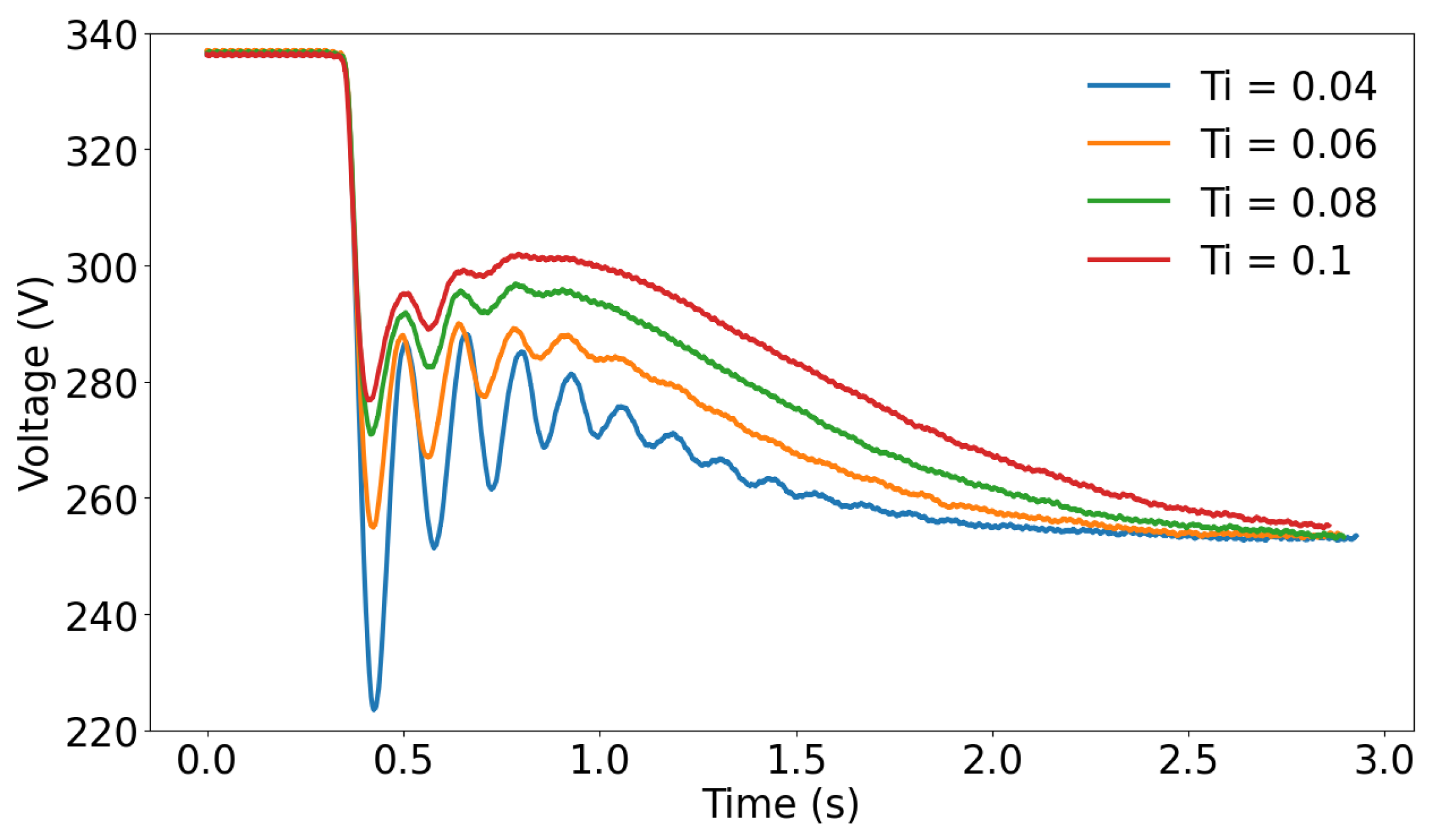
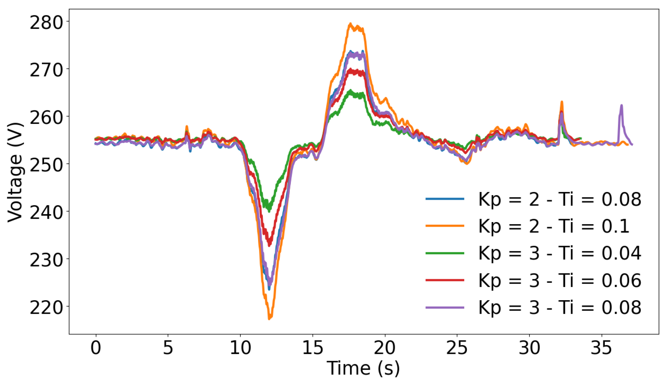
3.2.3. Influence of PI Tuning on the System Voltage Drop Simulation

Figure 24 shows the simulation of system voltage drop caused by Cloud 2 with different tuning parameters. As it can be seen, the waveform remains very similar, and larger values of $T_i$ make the amplitude larger, which must be avoided because it is closer to the minimum voltage value supported by the VFD.

There is something interesting in the figure. For the same value of $T_i$ and different $K_p$, the shape described is practically the same. This reinforces the hypothesis that the amplitude is directly related to $T_i$ and not to $K_p$.

3.3. About the Generalization of the Results

From the cloud samples collected during several months, the most critical ones (large irradiance drops in a very short time) have been chosen. It is known that PV power fluctuations are smoothed out with larger PV generators. Therefore, in real PVIS, which are larger than the system in our laboratory, the fluctuations will be less sharp. If the PI tuning method works with such demanding clouds, it will also work with smoother clouds. Therefore, this method is generalisable and useful for other PVIS sizes and for the PV power fluctuations that will be suffered by passing clouds.

4. Conclusions

Robustness is crucial in large-power stand-alone PVIS without batteries. This robustness depends fundamentally on the correct tuning of the PID control performed by the VFD.

The response of these systems is non-linear, so it is not possible to find a set of control parameters that ensure optimal operation under all conditions. Because of this, the tuning must be completed with a performance evaluation process. The most important evaluation test consists of checking the performance of the system in sudden drops of irradiance caused by passing clouds. This can only be done in very specific weather conditions, a circumstance that can cause significant delays in the system commissioning.

This paper shows a method to test the performance of the system under more favourable conditions of constant irradiance by using the feedforward control input. It has been described how the shape of this signal should be designed to simulate a certain irradiance curve profile. The algorithm designed to detect clouds and the subsequent characterization and analysis accomplished, have shown the relationship between irradiance drop and DC voltage drop. This allows to generate a disturbance in the system that causes the same effect as a real passing cloud.

A new tuning method that improves the AMIGO method used in the past, has also been proposed. This new method also makes use of the feedforward input, what avoid past stability problems when the system is being tuned.

Results of this method are quite promising. It has been possible to tune systems that were previously considered well tuned, improving their response. It is an iterative and simple method, which only requires a signal generator and oscilloscope to be executed.

The use of a triangular signal, whose derivative is a square signal is interesting to automate the tuning process in the future. These are very easy to generate and very suitable for mathematical analysis.

The fact that this method has been tested on a low-power PV generator, which is more sensitive to sudden drops in irradiance, and with the most critical clouds means that it can be extrapolated to much larger systems, whose response will be smoother. The application of this tuning and simulation method is expected to provide a significant improvement in performance and commissioning in real systems.

References

1. Langarita, R.; Chóliz, J.S.; Sarasa, C.; Duarte, R.; Jiménez, S. Electricity costs in irrigated agriculture: A case study for an irrigation scheme in Spain. Renew. Sustain. Energy Rev. 2017, 68, 1008–1019. [Google Scholar] [CrossRef]
2. Khiareddine, A.; Ben Salah, C.; Mimouni, M.F. Power management of a photovoltaic/battery pumping system in agricultural experiment station. Sol. Energy 2015, 112, 319–338. [Google Scholar] [CrossRef]
3. Das, M.; Mandal, R. A comparative performance analysis of direct, with battery, supercapacitor, and battery-supercapacitor enabled photovoltaic water pumping systems using centrifugal pump. Sol. Energy 2018, 171, 302–309. [Google Scholar] [CrossRef]
4. Bhayo, B.A.; Al-Kayiem, H.H.; Gilani, S.I. Assessment of standalone solar PV-Battery system for electricity generation and utilization of excess power for water pumping. Sol. Energy 2019, 194, 766–776. [Google Scholar] [CrossRef]
5. Almeida, R.; Carrêlo, I.; Carrasco, L.; Martínez-Moreno, F.; Narvarte, L. Large-scale hybrid PV-Grid irrigation system. SISIFO 2017, 5, 6. [Google Scholar]
6. Abella, M.; Lorenzo, E.; Chenlo, F. PV water pumping systems based on standard frequency converters. Prog. Photovolt. Res. Appl. 2003, 11, 179–191. [Google Scholar] [CrossRef]
7. Valer, L.R.; Melendez, T.A.; Fedrizzi, M.C.; Zilles, R.; de Moraes, A.M. Variable-speed drives in photovoltaic pumping systems for irrigation in Brazil. Sustain. Energy Technol. Assessm. 2016, 15, 20–26. [Google Scholar] [CrossRef]
8. Astrom, K.J.; Hagglund, T. Advanced PID Control; ISA: Research Triangle Park, NC, USA, 2009. [Google Scholar]
9. Brito, A.; Zilles, R. Systematized procedure for parameter characterization of a variable-speed drive used in photovoltaic pumping applications. Prog. Photovolt. Res. Appl. 2006, 14, 249–260. [Google Scholar] [CrossRef]
10. Fernández-Ramos, J.; Narvarte-Fernández, L.; Poza-Saura, F. Improvement of photovoltaic pumping systems based on standard frequency converters by means of programmable logic controllers. Sol. Energy 2010, 84, 101–109. [Google Scholar] [CrossRef]
11. Herraiz, J.I.; Fernández-Ramos, J.; Almeida, R.H.; Báguena, E.M.; Castillo-Cagigal, M.; Narvarte, L. On The Tuning and Performance Of Stand-Alone Large-Power Pv Irrigation Systems. Energy Convers. Manag. 2022, 13, 100175. [Google Scholar] [CrossRef]
12. Fernández-Ramos, J.; Narvarte, L.; López-Soria, R.; Almeida, R.; Carrêlo, I. An assessment of the proportional-integral control tuning rules applied to Photovoltaic Irrigation Systems based on Standard Frequency Converters. Sol. Energy 2019, 191, 468–480. [Google Scholar] [CrossRef]
13. Hägglund, T.; Åström, K.J. Revisiting the Ziegler-Nichols tuning rules for PI control. Asian J. Control 2002, 4, 364–380. [Google Scholar] [CrossRef]
14. Hägglund, T.; Åström, K.J. Revisiting the Ziegler-Nichols tuning rules for PI control—Part II the frequency response method. Asian J. Control 2004, 6, 469–482. [Google Scholar] [CrossRef]
15. Jewell, W.; Ramakumar, R. The Effects of Moving Clouds on Electric Utilities with Dispersed Photovoltaic Generation. IEEE Trans. Energy Convers. 1987, EC-2, 570–576. [Google Scholar] [CrossRef]
16. Jewell, W.; Unruh, T. Limits on cloud-induced fluctuation in photovoltaic generation. IEEE Trans. Energy Convers. 1990, 5, 8–14. [Google Scholar] [CrossRef]
17. Hoff, T.E.; Perez, R. Quantifying PV power Output Variability. Sol. Energy 2010, 84, 1782–1793. [Google Scholar] [CrossRef]
18. Lave, M.; Kleissl, J. Cloud speed impact on solar variability scaling—Application to the wavelet variability model. Sol. Energy 2013, 91, 11–21. [Google Scholar] [CrossRef]
19. Marcos, J.; Marroyo, L.; Lorenzo, E.; Alvira, D.; Izco, E. Power output fluctuations in large scale PV plants: One year observations with one second resolution and a derived analytic model. Prog. Photovolt. Res. Appl. 2011, 19, 218–227. [Google Scholar] [CrossRef]
20. Kuszamaul, S.; Ellis, A.; Stein, J.; Johnson, L. Lanai High-Density Irradiance Sensor Network for characterizing solar resource variability of MW-scale PV system. In Proceedings of the 2010 35th IEEE Photovoltaic Specialists Conference, Honolulu, HI, USA, 20–25 June 2010; pp. 283–288. [Google Scholar] [CrossRef]
21. Alam, M.J.E.; Muttaqi, K.M.; Sutanto, D. A Novel Approach for Ramp-Rate Control of Solar PV Using Energy Storage to Mitigate Output Fluctuations Caused by Cloud Passing. IEEE Trans. Energy Convers. 2014, 29, 507–518. [Google Scholar] [CrossRef]
22. Beltran, H.; Bilbao, E.; Belenguer, E.; Etxeberria-Otadui, I.; Rodriguez, P. Evaluation of Storage Energy Requirements for Constant Production in PV Power Plants. IEEE Trans. Ind. Electron. 2013, 60, 1225–1234. [Google Scholar] [CrossRef]
23. Han, X.; Chen, F.; Cui, X.; Li, Y.; Li, X. A Power Smoothing Control Strategy and Optimized Allocation of Battery Capacity Based on Hybrid Storage Energy Technology. Energies 2012, 5, 1593–1612. [Google Scholar] [CrossRef]
24. Kakimoto, N.; Satoh, H.; Takayama, S.; Nakamura, K. Ramp-Rate Control of Photovoltaic Generator With Electric Double-Layer Capacitor. IEEE Trans. Energy Convers. 2009, 24, 465–473. [Google Scholar] [CrossRef]
25. Darras, C.; Muselli, M.; Poggi, P.; Voyant, C.; Hoguet, J.C.; Montignac, F. PV output power fluctuations smoothing: The MYRTE platform experience. Int. J. Hydrogen Energy 2012, 37, 14015–14025. [Google Scholar] [CrossRef]
26. Marcos, J.; Marroyo, L.; Lorenzo, E.; Alvira, D.; Izco, E. From irradiance to output power fluctuations: The PV plant as a low pass filter. Prog. Photovolt. Res. Appl. 2011, 19, 505–510. [Google Scholar] [CrossRef]
27. Marcos, J.; Marroyo, L.; Lorenzo, E.; García, M. Smoothing of PV power fluctuations by geographical dispersion. Prog. Photovolt. Res. Appl. 2012, 20, 226–237. [Google Scholar] [CrossRef]
28. Lave, M.; Kleissl, J.; Arias-Castro, E. High-frequency irradiance fluctuations and geographic smoothing. Sol. Energy 2012, 86, 2190–2199. [Google Scholar] [CrossRef]
29. Perez, R.; Kivalov, S.; Schlemmer, J.; Hemker, K.; Hoff, T.E. Short-term irradiance variability: Preliminary estimation of station pair correlation as a function of distance. Sol. Energy 2012, 86, 2170–2176. [Google Scholar] [CrossRef]
30. Perpiñán, O.; Marcos, J.; Lorenzo, E. Electrical power fluctuations in a network of DC/AC inverters in a large PV plant: Relationship between correlation, distance and time scale. Sol. Energy 2013, 88, 227–241. [Google Scholar] [CrossRef]
31. Gilman, F.C. Testing Pumps as Fans and Fans as Pumps. J. Eng. Power 1968, 90, 140–142. [Google Scholar] [CrossRef]
32. King, J.A. Testing Pumps in Air. J. Eng. Power 1968, 90, 97–104. [Google Scholar] [CrossRef]
33. Bario, F.; Barral, L.; Bois, G. Air Test Flow Analysis of the Hydrogen Pump of Vulcain Rocket Engine. J. Fluids Eng. 1991, 113, 654–659. [Google Scholar] [CrossRef]
34. Choi, J.S.; McLaughlin, D.K.; Thompson, D.E. Experiments on the unsteady flow field and noise generation in a centrifugal pump impeller. J. Sound Vib. 2003, 263, 493–514. [Google Scholar] [CrossRef]
Figure 1. Cloud detection algorithm.
Energies 15 07191 g001
Figure 2. Cloud 1 (50.59% irradiance drop): irradiance fluctuation and corresponding system voltage disturbance.
Energies 15 07191 g002
Figure 3. Cloud 2 (59.41% irradiance drop): irradiance fluctuation and corresponding system voltage disturbance.
Energies 15 07191 g003
Figure 4. PID diagram with feedforward input.
Energies 15 07191 g004
Figure 5. Cloud 1: Similarity of irradiance and frequency response shapes.
Energies 15 07191 g005
Figure 6. Cloud 2: Similarity of irradiance and frequency response shapes.
Energies 15 07191 g006
Figure 7. Feedforward signal, equivalent to the normalized and inverted irradiance, used to simulate the system voltage drop corresponding to Cloud 2.
Energies 15 07191 g007
Figure 8. Voltage and derivative of irradiance comparation.
Energies 15 07191 g008
Figure 9. Relation between system voltage drop and feedforward signal amplitude for Cloud 1.
Energies 15 07191 g009
Figure 10. Relation between system voltage drop and feedforward signal amplitude for Cloud 2.
Energies 15 07191 g010
Figure 11. System voltage disturbances produced by different amplitudes of the feedforward signal for Cloud 1.
Energies 15 07191 g011
Figure 12. System voltage disturbances produced by different amplitudes of the feedforward signal for Cloud 2.
Energies 15 07191 g012
Figure 13. System voltage disturbance with real and simulated Cloud 1.
Energies 15 07191 g013
Figure 14. System voltage disturbance with real and simulated Cloud 2.
Energies 15 07191 g014
Figure 15. System voltage disturbance with a triangular feedforward signal, different K p and T i = 0.1 .
Energies 15 07191 g015
Figure 16. System voltage disturbance with a triangular feedforward signal, different K p and T i = 0.2 .
Energies 15 07191 g016
Figure 17. System voltage disturbance with a triangular feedforward signal, different T i and K p = 3 .
Energies 15 07191 g017
Figure 18. System voltage signal at the starting phase with K p = 1 and different T i .
Energies 15 07191 g018
Figure 19. System voltage signal at the starting phase with K p = 2 and different T i .
Energies 15 07191 g019
Figure 20. System voltage signal at the starting phase with K p = 3 and different T i .
Energies 15 07191 g020
Figure 21. System frequency signal at the starting phase with K p = 1 and different T i .
Energies 15 07191 g021
Figure 22. System frequency signal at the starting phase with K p = 2 and different T i .
Energies 15 07191 g022
Figure 23. System frequency signal at the starting phase with K p = 3 and different T i .
Energies 15 07191 g023
Figure 24. System voltage disturbance simulated for Cloud 2 with different PI constants.
Energies 15 07191 g024