1. Introduction
Accurate determination of heat transfer coefficient is imperative in order to design efficient heat exchangers. Gas turbine blade is a classic example of an advanced heat exchanger that is subjected to hot gases (~1700 °C) exiting the combustor section, and where coolant bled off from the compressor section (~700 °C) is routed through the complex internal cooling passages inside the hollow blades [
1]. A comprehensive information on state-of-the-art gas turbine airfoil cooling can be found in [
2]. Impingement cooling is typically employed in the leading-edge region of the gas turbine blade, which is subjected to high heat loads due to stagnation of incoming hot gases from the combustor. Typically, a single row of jets spanning the blade height is used to allow coolant to impinge from the internal side [
3]. Impinging jets are also arranged in an array form for potential application in the mid-chord region in turbine airfoils. Benchmark correlations on single jet impingement and array jet impingement are provided in [
4,
5,
6], where experiments were carried out under steady-state conditions. In [
4,
5,
6], metal stripes were subjected to constant heat flux, and with the knowledge of metal temperature (measured by thermocouple) and reference fluid temperature, the convective heat transfer coefficient was determined. This method provides regionally averaged heat transfer data that do not necessarily capture the local effects of the impinging jets. With the evolution of advanced thermal diagnostic techniques, researchers have developed heat transfer measurement techniques based on liquid crystal thermography (
LCT) and infrared thermography (
IRT) which provides surface temperatures in high spatio-temporal resolution.
Some of the earlier investigations on
LCT to determine local
h using 1-D semi-infinite assumption were carried out by [
7,
8,
9,
10]. Comprehensive details about liquid crystal basics [
11], operating principles [
11],
LC-based measurement techniques [
12] can be found in the above references. Treatment of target surface as a 1-D semi-infinite medium has been a central assumption in the above techniques [
12]. In such short-duration experiments, a sudden change in fluid temperature is achieved, which essentially drives the solid temperature such that all the pixels in the region of interest cross the liquid crystal color change band. With the knowledge of at least one time-temperature pair, an inverse heat transfer technique is adopted to calculate the convective heat transfer coefficient. With the treatment of solid as a 1D semi-infinite medium, the analytical solution of surface temperature evolution with time, is used under the assumption of time-invariant fluid temperature, and an iterative method is adopted to find the value of
h for each pixel based on its respective time taken to reach a certain temperature. Since, in actual experiments, obtaining a perfect step change in fluid temperature is not possible, a Duhamel’s superposition principle is applied on the analytical solution of wall temperature evolution for a 1D semi-infinite solid, to account for the temporal variation of the fluid temperature.
Although there have been numerous investigations on the employment of 1-D semi-infinite model using either
LCT or
IRT, very few studies have been carried out on the critical assessment of this assumption and the extent to which it can yield in reasonably accurate
h values, under different flow scenarios. Lin and Wang [
13] presented a technique for determining
h by modeling 3-D heat diffusion through an inverse heat transfer technique. The authors [
13] used liquid crystal thermography for the determination of time taken to reach a particular wall temperature and then used a guess heat transfer distribution to build a revised time matrix and upon the comparison of the built and actual time matrix, subsequent corrections in local
h were applied. Above process was repeated until the specified convergence criteria on time matrix (through 3-D heat diffusion based on
h-guess and actual time matrix) was met. This technique, however, was different from the typical transient
LCT experiment as in [
10] where a step change in fluid temperature is required at the start of the experiment and this results in rise or fall in the solid surface temperature. In [
13], the test surface was heated suddenly and air was supplied at laboratory ambient conditions. The authors in [
13] found that significant differences between the 3-D and 1-D model can be observed particularly at the stagnation regions and the low heat transfer regions between the adjacent jets, in a typical array jet impingement configuration. Heat transfer coefficient obtained through 1-D model was found to be higher by ~20% higher than that obtained from 3-D model in the first row of array jet impingement under maximum crossflow condition. Nirmalan et al. [
14] carried out jet impingement experiments on metallic target and compared the lumped capacitance- (0-D) based
h with that of the 3-D heat diffusion model. The authors found that
h found with 3-D model was ~25% higher than the lumped capacitance model.
More recently, Brack et al. [
15] evaluated transient infrared and liquid crystal thermography techniques under 1-D and 3-D heat diffusion modeling for flow over a flat surface and flow over a vortex generator. The benefits of using infrared thermography were demonstrated through the presentation of a time-accurate heat transfer coefficient, whereas the
LCT yields one value of
h for a given pixel of interest. In both techniques, it was observed that the
h obtained through 1-D heat diffusion was higher than that obtained from 3-D heat diffusion and that
h1d continued to change with time while
h3d settled to a constant value. The configuration with larger gradients in
h had larger discrepancies between
h obtained through 1-D and 3-D methods. Further, fast transient experiments had low differences between
h through 1-D and 3-D calculations. Brack et al. [
16] presented a comprehensive study on the differences between local
h obtained through 1-D and 3-D heat conduction models where a sample impingement configuration (along with five other
Bi distributions) was analyzed for different mainstream temperature transient evolution. The authors presented a local distribution of the discrepancy in the form of
, where
is the true Biot number (
Bi) distribution. To the best of our knowledge, this was the first time, a local map of
was presented. It was shown that in the regions between adjacent jet footprints (low heat transfer zones), 1-D method can overpredict the heat transfer coefficient by ~8% and that the
at the stagnation region was below zero (indicating
). Ahmed et al. [
17] carried out similar analysis following the approach in [
13] for
h determination through 3-D calculations for jet impingement case. The
h-guess method was adopted, and the initial guess was improved after each iteration by comparing the time matrices obtained experimentally and computationally. The authors considered a single row of impinging jets typical of maximum crossflow condition and carried out 1-D and 3-D computations for
h determination and observed that
h obtained through 3-D computations following the approach mentioned in [
13] was consistently higher than that obtained through 1-D calculations. Literature review on
h1d and
h3d deviations suggests that they are dependent on flow configuration and that most studies have been carried out theoretically except [
15,
17]. However, the methodologies adopted to determine the
h1d and
h3d deviations in [
15] and [
17] were different while both studies indicate that large deviations can be observed in cases where gradients in “true h” is large.
To this end, we recognize that the topic of the 1-D versus 3-D heat diffusion computational approach is important since the differences in
h between these two approaches can be significant at times, and these differences are often ignored. In this paper, we present a simple exercise to showcase the discrepancy
as in [
16]) for the case of jet impingement. Three case studies are considered, (a) single jet, (b) array jet (theoretical distribution), and (c) array jet (experimental distribution). The reason behind these choices is to cover different aspects such as monotonically decreasing
h distribution (single jet) with steady gradient, sinusoidal variations in
h with sharp gradients with analysis on local
h variation along the line joining jet centers (high heat transfer zones, similar to [
17]) and line bisecting the line joining two adjacent jet centers (low heat transfer zones). Further, an array of experimentally obtained
h distribution [
18] is used to demonstrate the practicality of the 1-D and 3-D computational approaches and how the
local variation compares between theoretical and experimental
h distributions. Above case studies are evaluated for three different fluid temperature time evolution profiles that are representative of high-performance mesh heaters (similar to ideal step change), moderately fast step change (similar to most transient experiments) and a slow transient (also observed in a few studies). The relative error
infact depends on several variables partaking in the transient experiments that none of the prior studies reviewed above have explored. The conclusions on the nature of
is subjective and warrants a comprehensive investigation. This paper attempts to cover the above issue and also provide recommendations for best practices in the design of transient experiments intended toward the determination of local
h.
2. Case Study
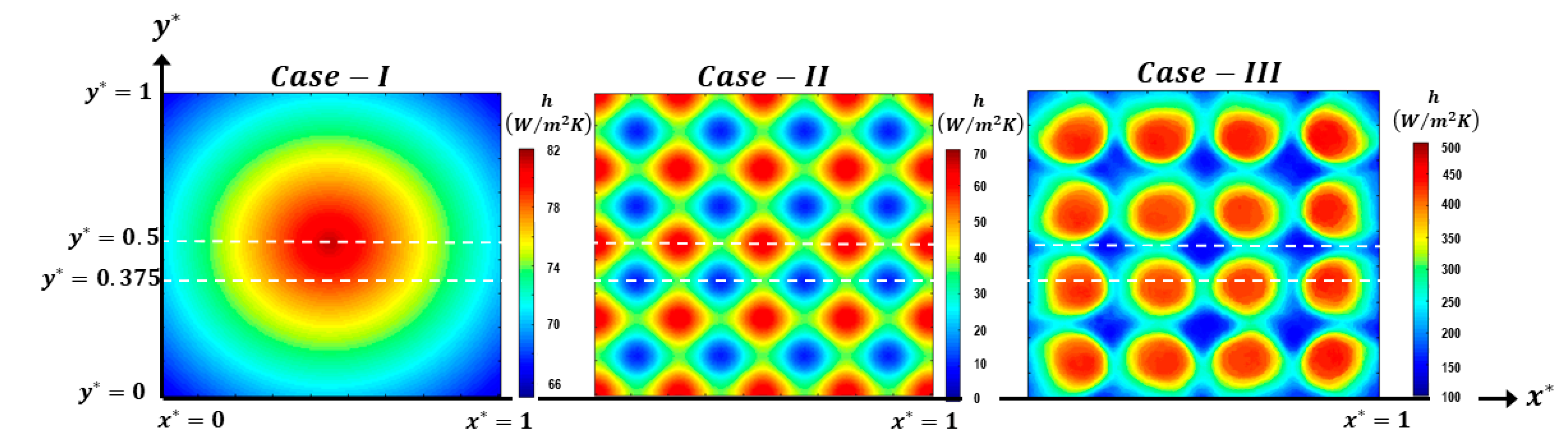
In this paper, three different cases of jet impingement have been studied as mentioned above. In each of the case, a true
h (
distribution is considered as a first step and is used subsequently for further computational heat transfer calculations.
Figure 1 shows the true
h distributions of each case.
The single jet case heat transfer coefficient distribution was obtained from the correlation prescribed by Goldstein and Behbahani [
4], where the convective heat transfer coefficient was given as,
where A = 4.577, B = 0.4357,
n = 1.14. Above correlation was prescribed for nozzle aspect ratio of 12. We have studied
h obtained from Equation (1) for Re = 20,000 and 35,200. The target area had a dimension of 76.2 mm × 76.2 mm and a thickness of 12.7 mm. The jet diameter was 25.4 mm. The solid target was discretized into 181 × 181 × 41 nodes and this choice is based on a grid convergence study. The Case II heat transfer coefficient distribution was obtained from Equation (2) and was based on one of the
Bi-distribution simulated in [
16].
In Equation (2), a = 36.84, b = 13.16, c = 13.16, d = 8.1, values were used to generate the “true h” or simply
h3d (from hereafter) distribution for Case II. The Case III data were extracted from Singh and Ekkad [
18] for the moderate crossflow scheme at z/d = 1. Note that the Case III distribution is being used here as
h3d distribution to facilitate discussion on a typical experimental 2D heat transfer distribution that may not be as smooth and well-defined as the theoretical ones (case I and II). In [
18], the authors have reported the detailed heat transfer coefficients based on 1-D semi-infinite conduction modeling but in this paper, the extracted
h is serving a different purpose.
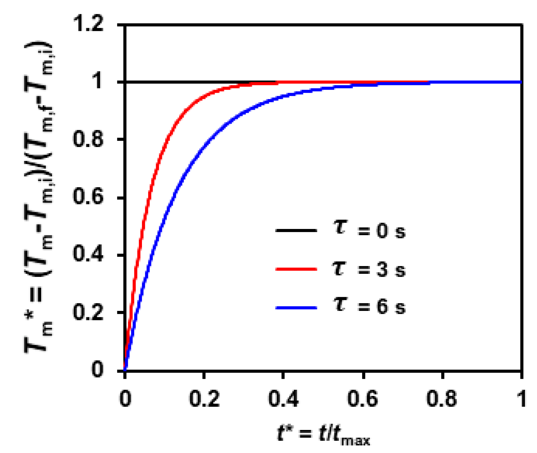
Further, three different mainstream temperature evolutions (typical of heated runs) were studied.
Figure 2 shows the three different evolution cases, where the temporal evolution is given by,
The initial temperature for (step change) case was 60 ° C, whereas the initial temperature for the (moderately fast transient) and (slow transient) was 20 ° C.
Data Reduction Methods
The analysis on the differences between
h3d and that obtained by modeling heat diffusion as strictly one-dimensional (
h1d) has been carried out for different data reduction possibilities.
Table 1 shows the details of different methods studied in this paper. This paper essentially covers different possible data reduction procedures typically employed in transient heat transfer experiments based on
LCT or
IRT.
3. Computational Procedure
This paper is aimed toward quantifying the local differences between the
h3d and
h1d, presented as
. Initially, starting with a known
h distribution (
, the three-dimensional heat diffusion equation (Equation (4)) is used to calculate the temporal evolution of each elements’ temperature in the 181 × 181 × 41 grid. Note that Equation (4) is true when there is no volumetric (internal) heat generation.
The top surface of the solid was subjected to convective-type boundary condition whereas the backside of the solid was maintained at a fixed temperature (. The remaining four side edges were set as adiabatic. This boundary condition is typical of the short-duration transient LC or IR experiments carried out on clear acrylic where the experimental duration is kept well below the time taken to penetrate the entire solid thickness resulting in the violation of the backside boundary condition of time-invariant wall temperature during the transient experiment.
The analytical solution for surface temperature evolution with time for convection-type boundary condition in 1-D semi-infinite model is given by Equation (5) and is obtained under the above assumption that backside temperature stays fixed at
and mainstream temperature is constant. However, our computational methodology is not based on Equation (5) and is entirely based on the finite difference method.
where
.
A computationally inexpensive explicit formulation was adopted to solve the surface and internal element temperatures of the solid where the 3-D heat diffusion given by Equation (4) was solved for each known
h distribution at the surface [
19]. This 4-D temperature matrix was considered to be equivalent to actual transient experiments carried out on clear acrylic with heat diffusion into the thickness of the solid as well as in lateral directions. The 4-D temperature matrix was built for a time duration of 45 s (
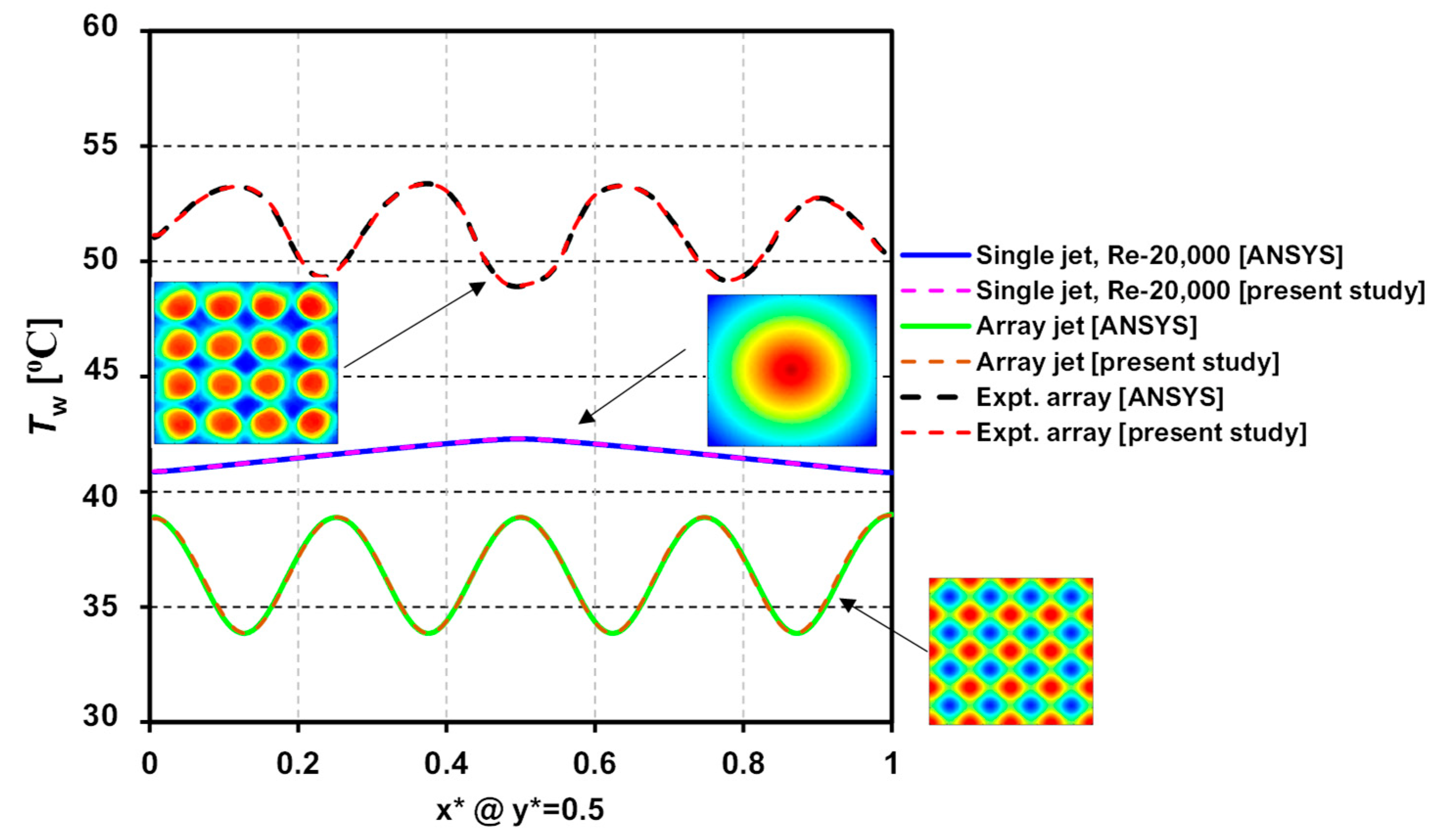
). The in-house explicit formulation was also compared against ANSYS FLUENT solver by modeling the exact same solid with the same spatial and temporal discretization, and a comparison for all three cases is shown in
Figure 3, where surface temperature evaluated at
is plotted at the centerline of the surface. The agreement between in-house code and FLUENT was ~100%, and
Table 2 shows the percentage deviations at selected locations, between the in-house code and the FLUENT code. In this paper, we have used our in-house code for both 3-d and 1-d computations, as it can be potentially applied to more complex initial and boundary conditions.
Once the 4-D temperature matrix is built, the surface temperature information is then extracted. This surface temperature is considered to be representative of a typical
TLC or
IRT test. Now, in the transient
LC approach, a certain reference wall temperature is tracked for each pixel and the time taken for that pixel to reach the reference temperature is stored in a time matrix. This time matrix is then used in Equation (5) to iteratively determine the only unknown
h (=h
1d). If the mainstream temperature varies with time, Equation (5) is further modified by using Duhamel’s superposition principle, for details see [
12]. In our 3-D heat conduction solver, the time variation of mainstream temperature feature is included.
In this paper, to calculate
, firstly a time matrix is built for Methods A–C (
Table 1) corresponding to method-specific wall temperature to be tracked. In method D, a certain time matrix was taken, and the corresponding reference wall temperature was determined/tracked. In all methods and configurations,
was then found using the method detailed in [
20] and is not repeated here in the interest of brevity. With the knowledge of
, the local difference
was calculated and reported both in local and line variation formats.
4. Results and Discussion
In this section, we present our analysis on
and
obtained for the four methods (A–D) outlined in
Table 1.
4.1. Method A: and Deviations at a Fixed ,
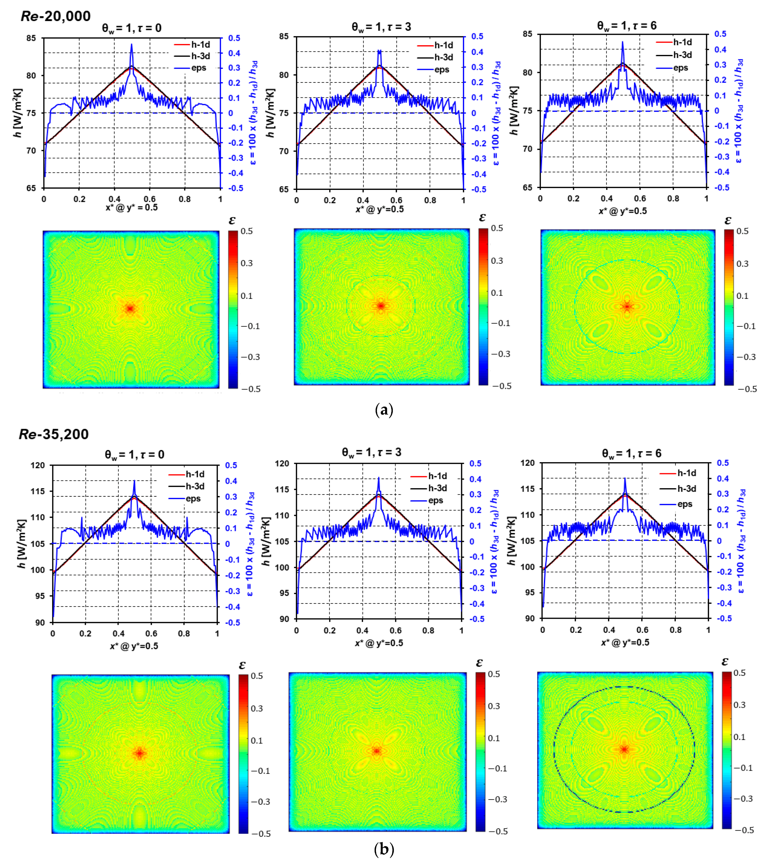
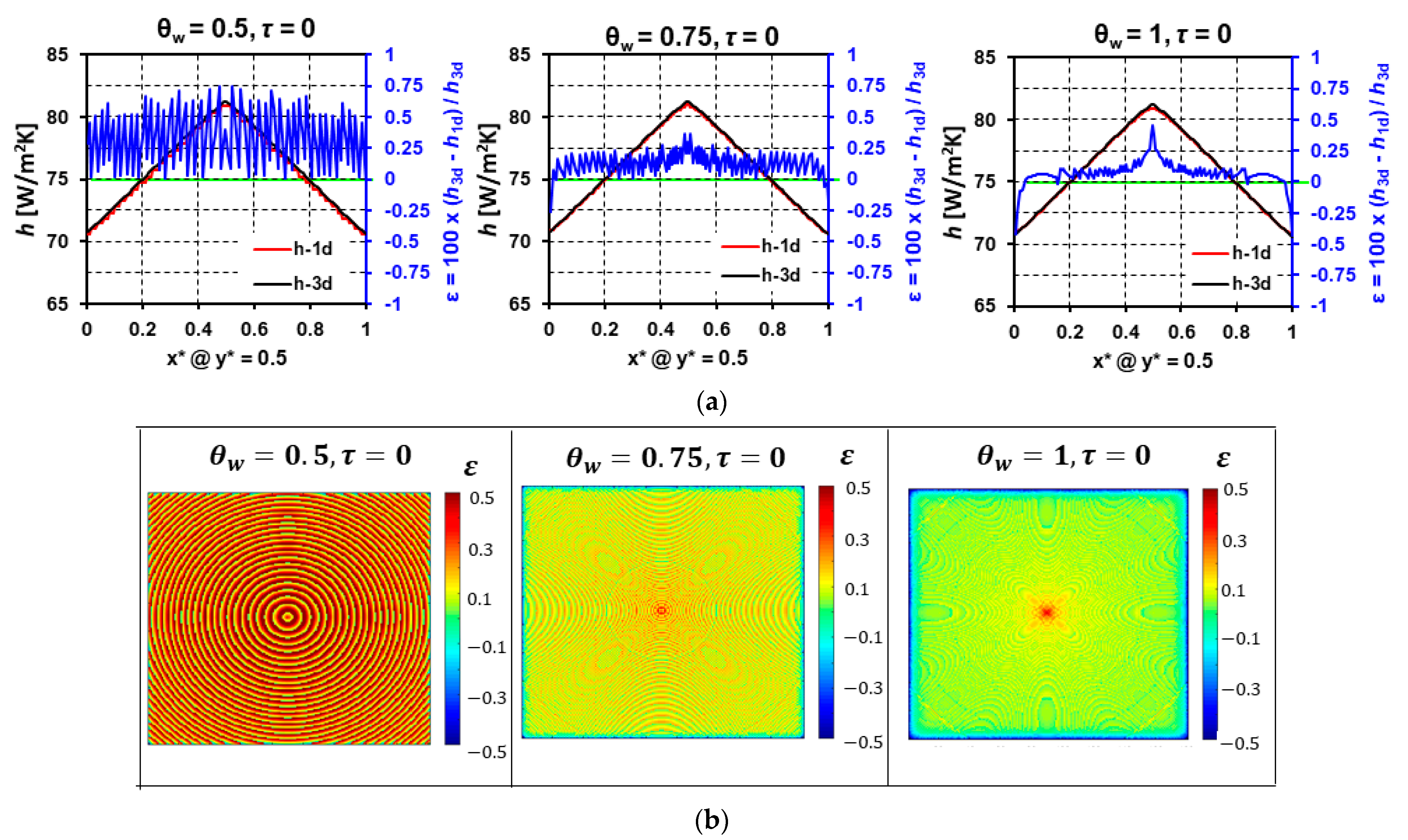
This section presents the results obtained from the above procedure for the three cases. Firstly, for the single jet case,
Figure 4 shows the comparison of
and
along with the
variation at the surface centerline. For
Re = 20,000 cases and the step change in the mainstream temperature, the
was found to be higher than
at the jet stagnation, whereas the 1-D and 3-D
h differences in radially outward direction were minimal.
Toward the edge of the solid (treated as adiabatic), the trends, however, flip. Similar trends were observed for the moderate and slow transients, with increasing differences and , where the jet stagnation region uncertainties continue to drop and going below zero. It can be concluded that and differences depend upon the local gradient in h as well as the mainstream temperature evolution. The scatter in is attributed to the grid resolution. To further explore the h gradient effect, we also investigated higher Re = 35,200 and found that the trends were similar to Re = 20,000.
In contrast to above finer points about the differences between and , it should be noted that the % differences were between −0.2% to 0.3% or ~ around the zero error. To a heat exchanger designer, these differences are negligible in comparison with the measurement uncertainties itself (typically ~10% for TLC experiments). Above conclusions are true only for the straightforward case of single jet with monotonically decreasing h from the jet footprint center.
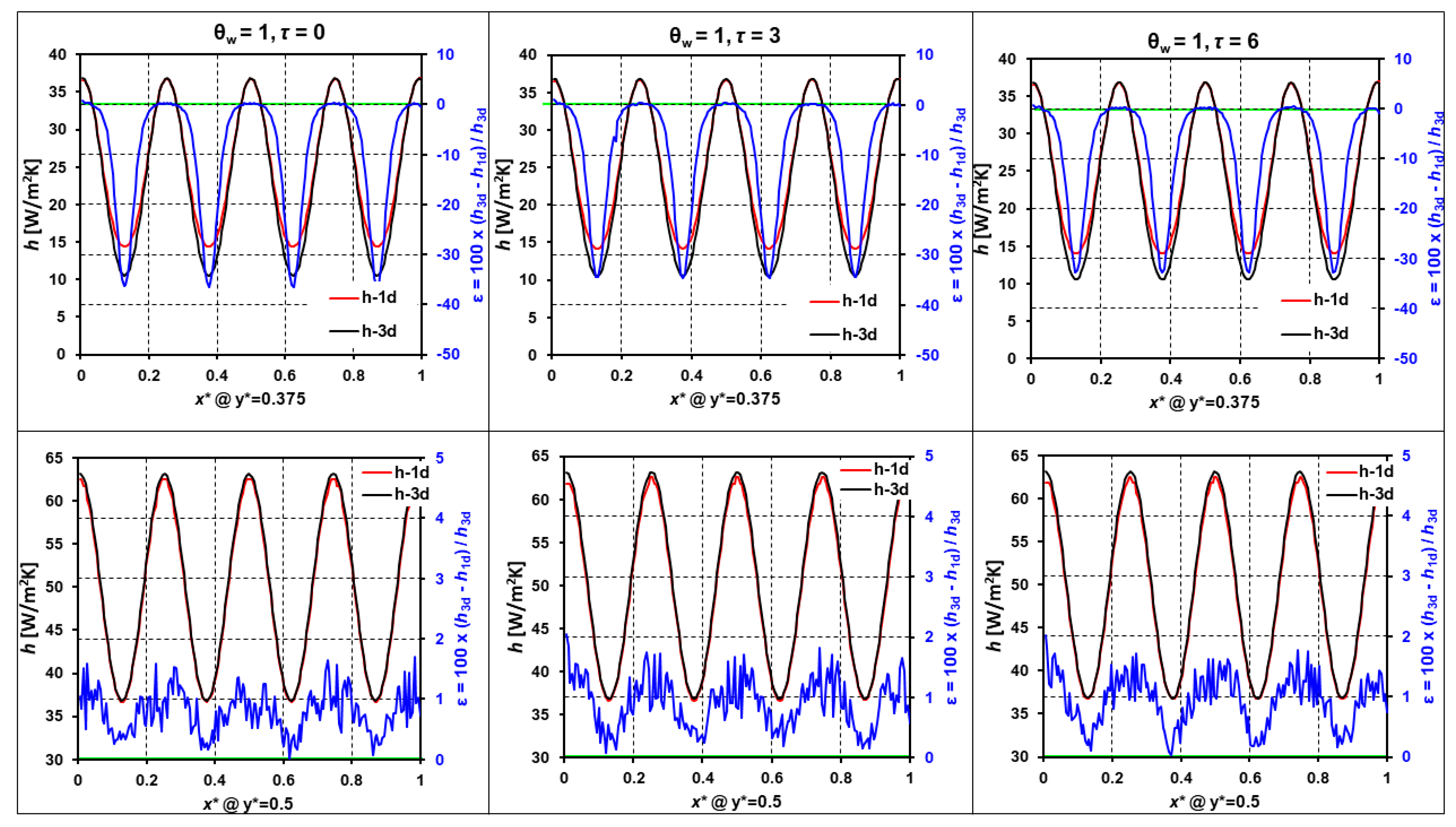
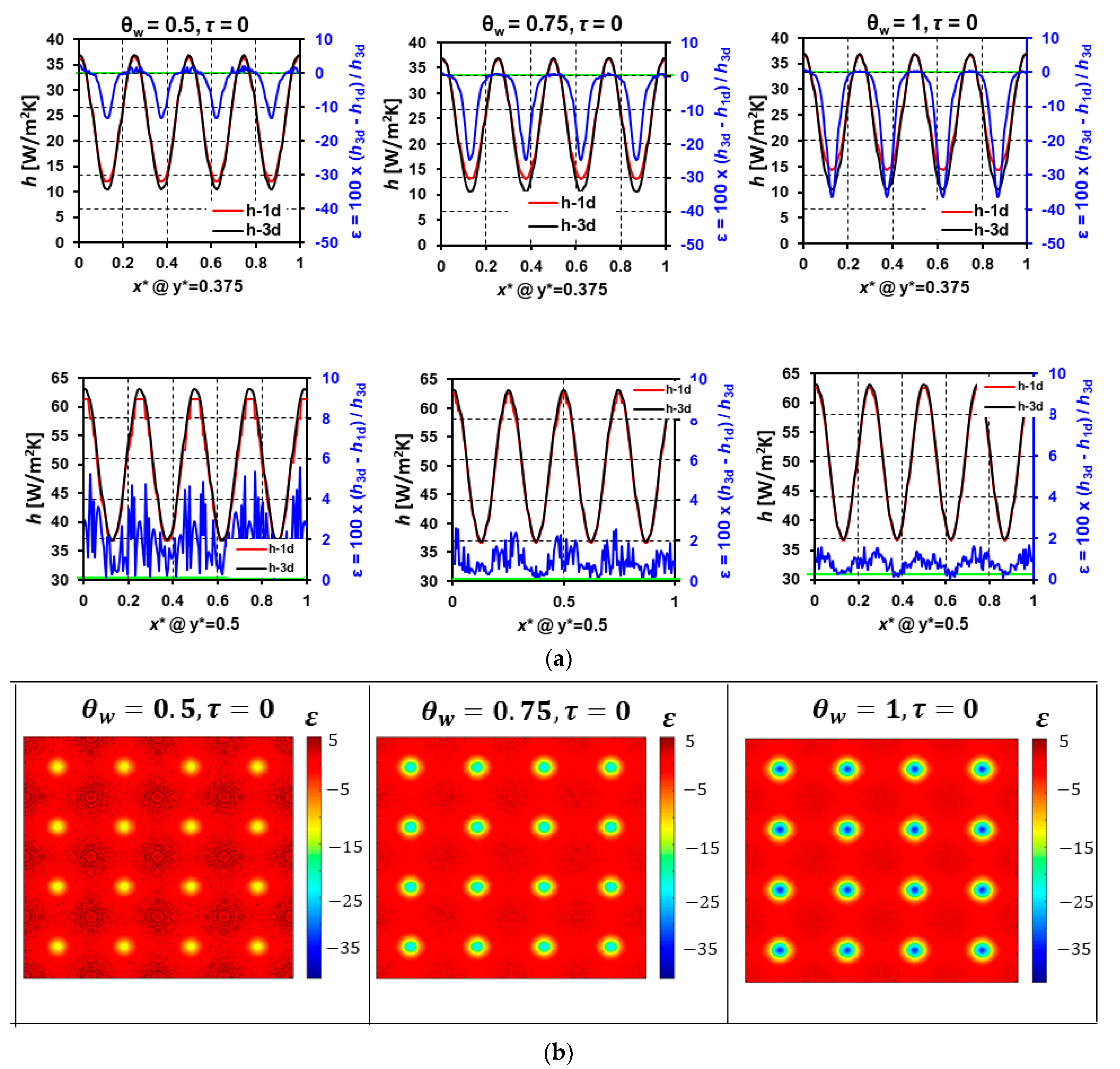
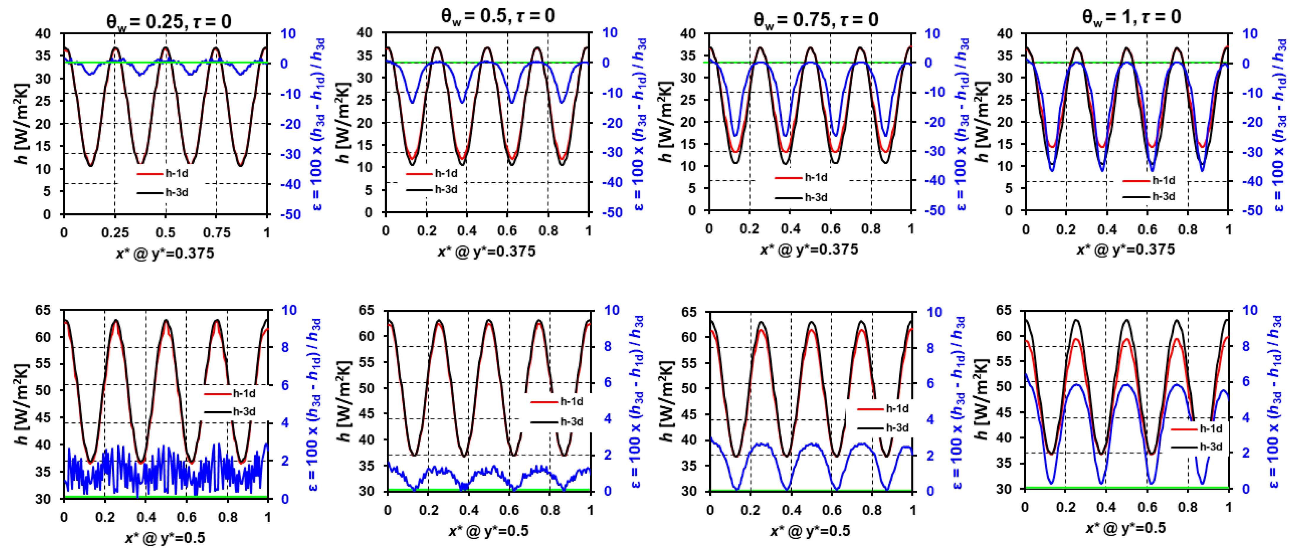
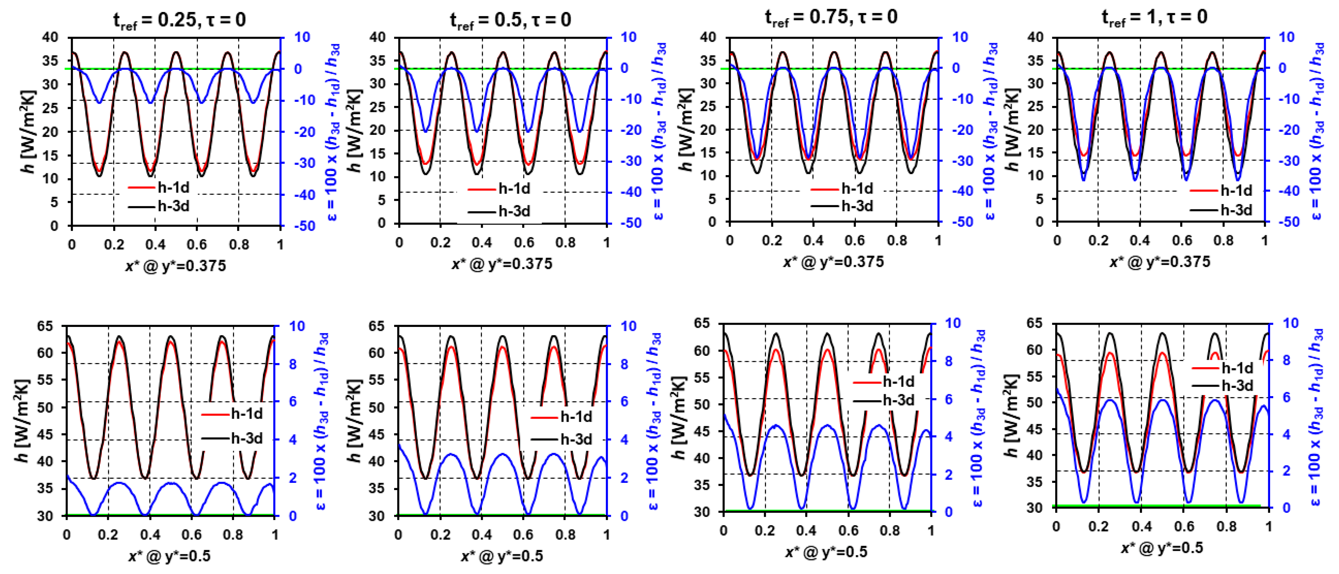
For the array jet impingement (theoretical distribution) case, local
h has been plotted with x* at two different y* locations of 0.375 and 0.5, where y* = 0.375 line passes through the low heat transfer regions, which typically occur in the gaps between adjacent jets while y* = 0.5 passes through the stagnation regions (
Figure 5). The low heat transfer line (y* = 0.375) had a significant difference between
and
particularly in the regions with the lowest heat transfer, where the 1-D model over-calculated the local
h by as much as 35% in reference to the
h3d. However, at the relatively high heat transfer regions (still on the low heat transfer line, y* = 0.375),
and
yield in nearly similar local
h, with
slightly greater than
.
This difference, however, was negligible in reference to the low heat transfer region discrepancies. This trend is a major takeaway from this study that 1-D conduction models should be applied carefully as they can sometimes lead to significantly overpredicted cooling rates in local heat transfer zones. Discrepancies between
and
for high heat transfer line (y* = 0.5), on the other hand, were very different when compared to y* = 0.375. 1-D modeling yields near accurate
h values for line intersecting stagnation points, where
was consistently higher (~1%) than
. A similar trend was observed in [
17].
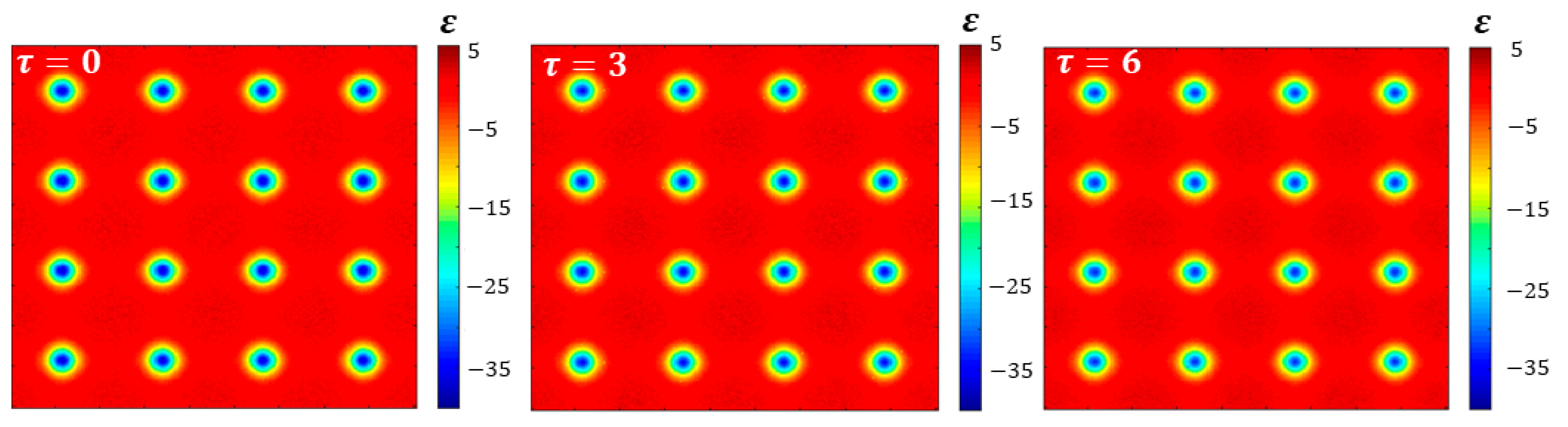
Figure 6 shows the local deviation between
and
and it can be observed that the low heat transfer regions exhibited large discrepancies as compared to the jet stagnation regions (high heat transfer zones). In other words, a 2-D
h distribution obtained from 1-D semi-infinite heat conduction model may give the wrong message that if such a cooling system is adopted, the resultant thermal stresses will be lower since the gradient in
h obtained would be smaller as compared to the
h obtained via modeling three-dimensional heat diffusion. Note that the mainstream temperature evolution did not have a very prominent effect on the
and
deviations.
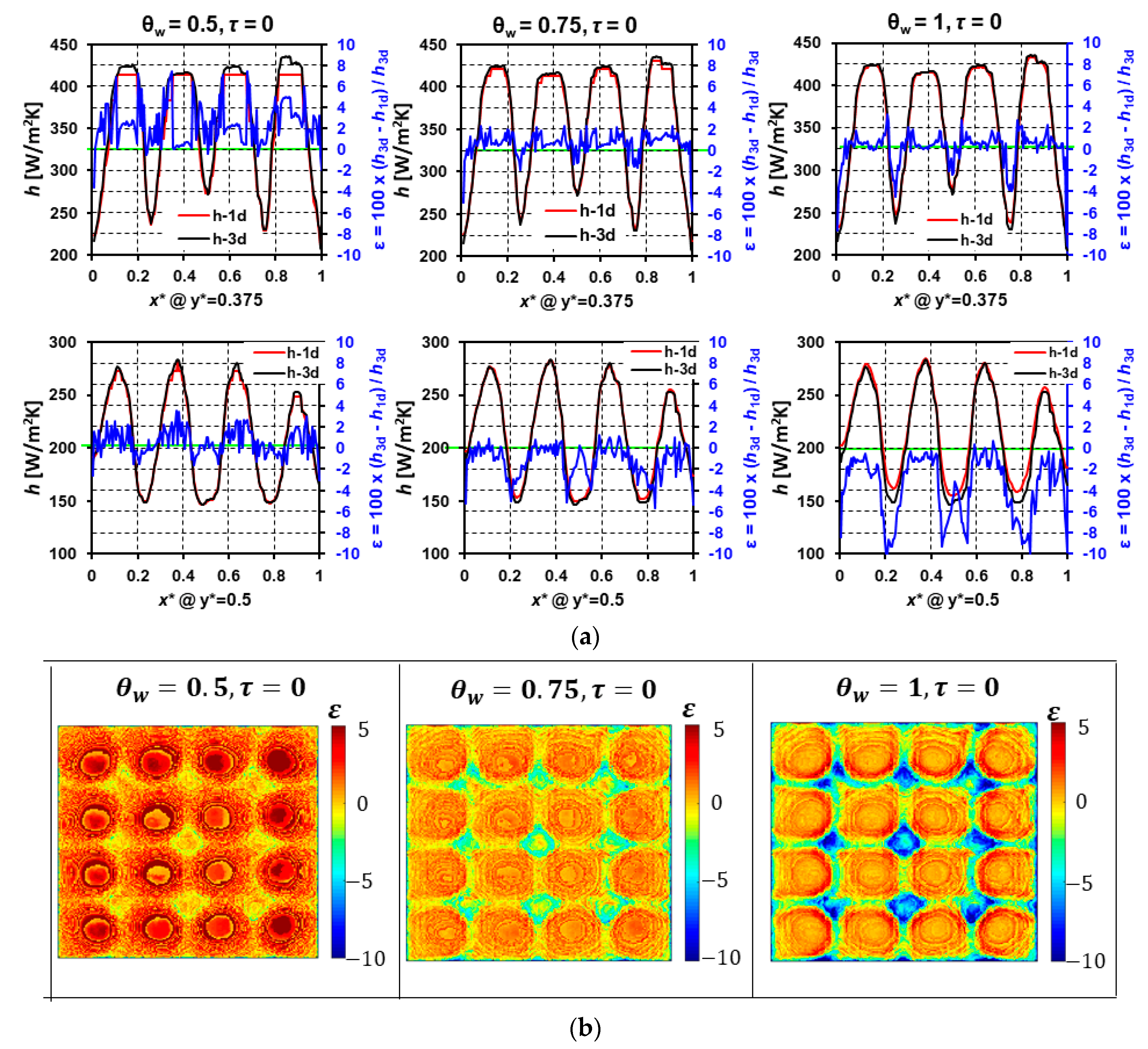
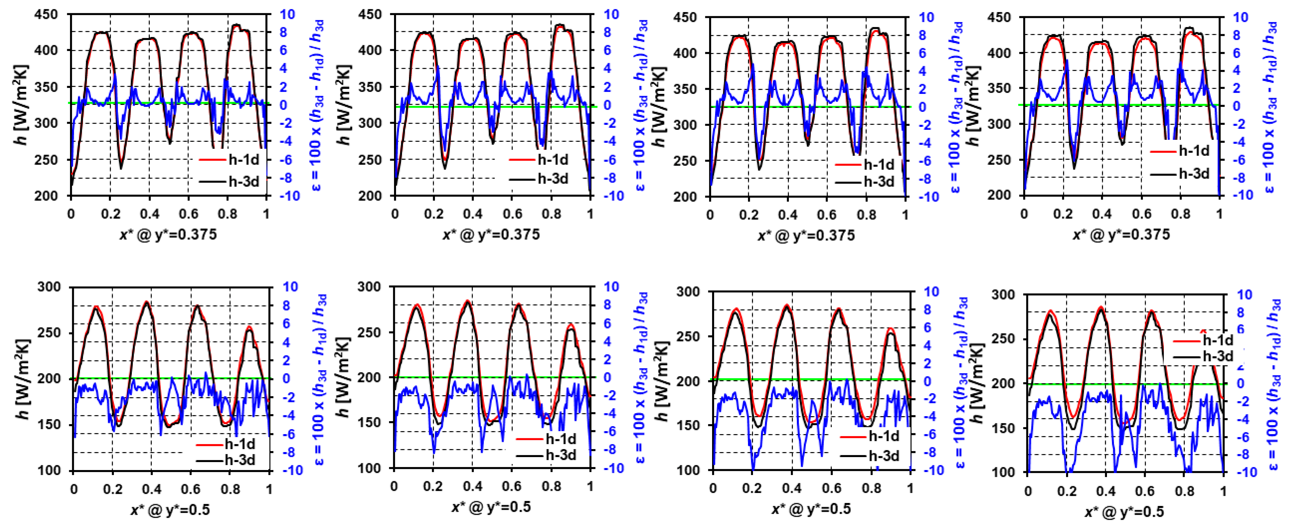
The last case (III) is based on
h distribution extracted from Singh and Ekkad [
18], where the authors investigated target wall heat transfer for an impingement-effusion system for low jet-to-target spacing. The jet-to-jet spacing was six times the jet diameter, hence providing significant room for low heat transfer regions, which is the ideal case for this study since we learned from the theoretical array jet impingement distribution that low heat transfer zones exhibit significant discrepancies between
and
. Note that
h presented in [
18] was determined through modified Equation (5), where heat diffusion was considered as 1-D. Here we are using the
h presented in [
18] as a realistic 2D distribution to perform
and
deviation analysis.
The experimentally obtained h distribution facilitates much-needed discussion on the discrepancy between and since the 2D distribution, in this case, has local fluctuations in h as well, due to the several factors involved in experiments such as inherent surface roughness on “smooth” targets, liquid crystal paint spray-induced roughness, camera resolution, etc. These local fluctuations in h may have a profound effect when lateral conduction is considered, and hence, Case III has been considered in this demonstration study. To the best of the author’s knowledge, such a local discrepancy between and for an experimental h distribution has not been presented before.
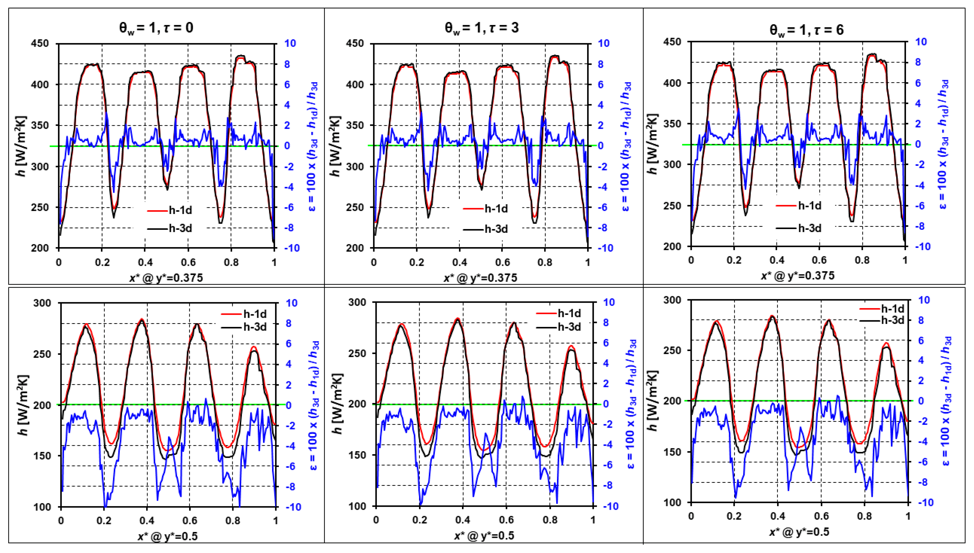
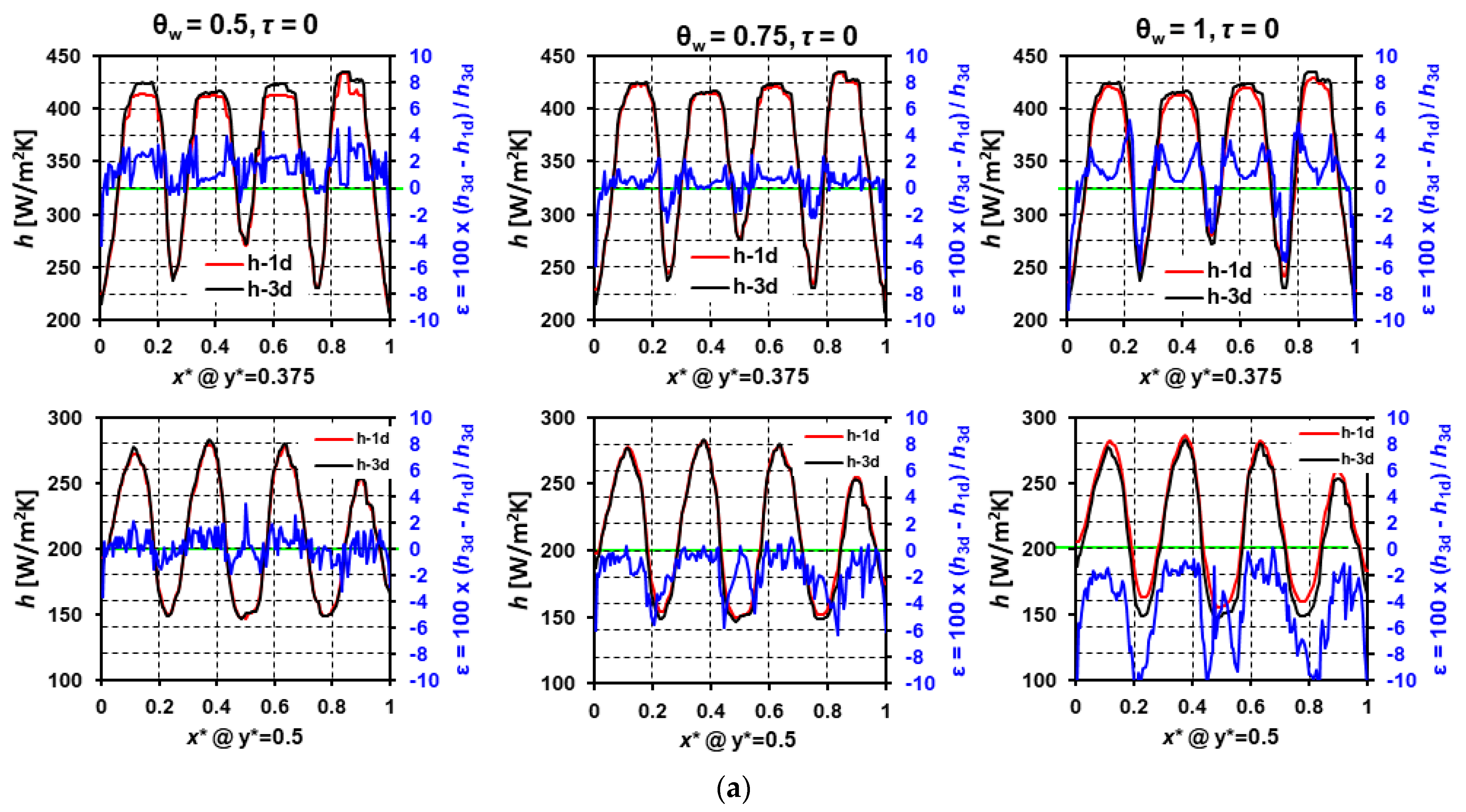
Figure 7 shows the
and
deviations for Case III, where the line y* = 0.375 now corresponds to the high heat transfer zones and y* = 0.5 to the low heat transfer zones (
Figure 1). Similar to Case II, the low heat transfer line had significant differences between
and
, where
yielded in ~10% higher values of
h in the low heat transfer zones falling on the low heat transfer line y* = 0.5. The discrepancy in Case III is lower than in Case II; however, the values depend upon several factors involved in the transient experiments.
It is pointed out that local fluctuations in real
h values may have a noteworthy impact on the
and
deviations. On the high heat transfer line y* = 0.375, the
and
deviations were almost non-existent, with
slightly higher than
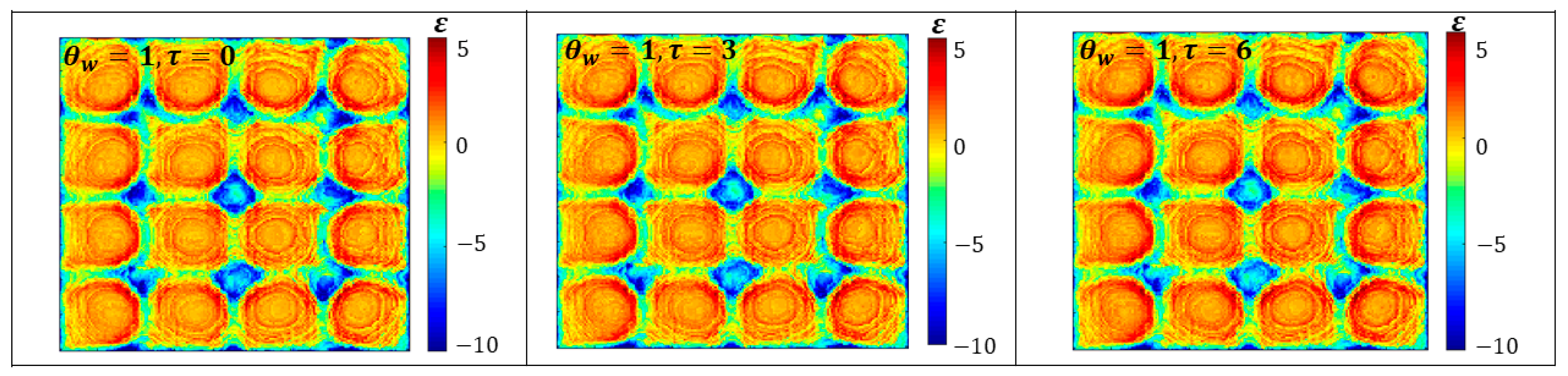
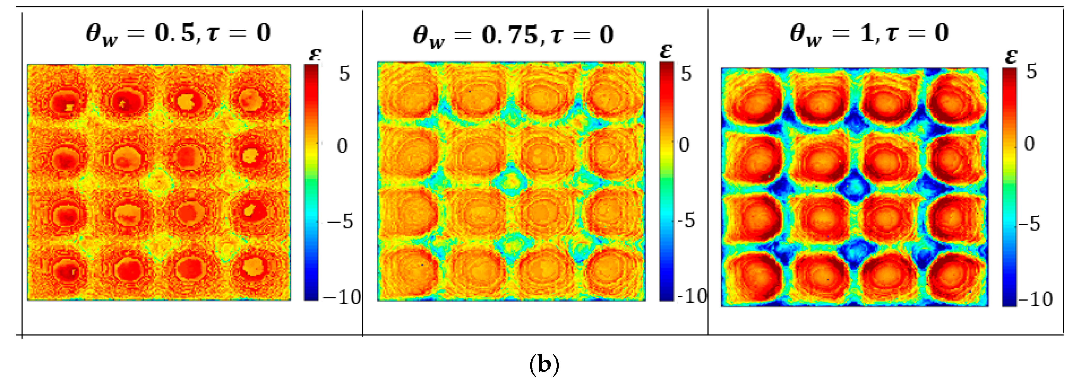
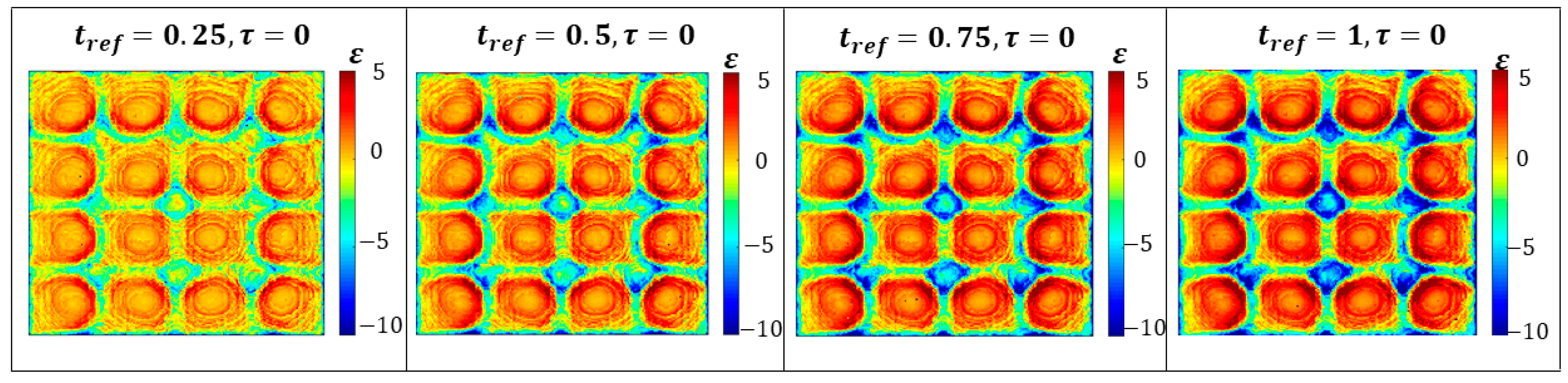
at the stagnation regions. From the contour of
and
deviations (
Figure 8), it is observed that regions with smaller gradients in local true
h values, whether it corresponds to low or high heat transfer zone, the
and
deviations are nearly zero and can be safely ignored from the cooling design point of view. Note that the mainstream temperature time constant did not have a prominent effect on the
and
deviations in this case as well. We now explore other methodologies (B–D) that could be adopted for
h determination for the step change in mainstream temperature case only (i.e.,
τ = 0).
4.2. Method B: and Deviations at a Fixed ,
In
Section 4.1, we presented cases with
, which is tracking the same wall temperature for each pixel, and the wall temperature, in that case, was the global minimum wall temperature at the end of the transient experiment/simulation (
tmax = 45 s). In this section, we present the effect of the choice of wall temperature to be tracked on the differences between
and
. To this end, three different cases have been considered, which correspond to all pixels tracked to
. Note that
for
has already been presented in
Section 4.1, but here we have presented it again to facilitate comparisons for different
values.
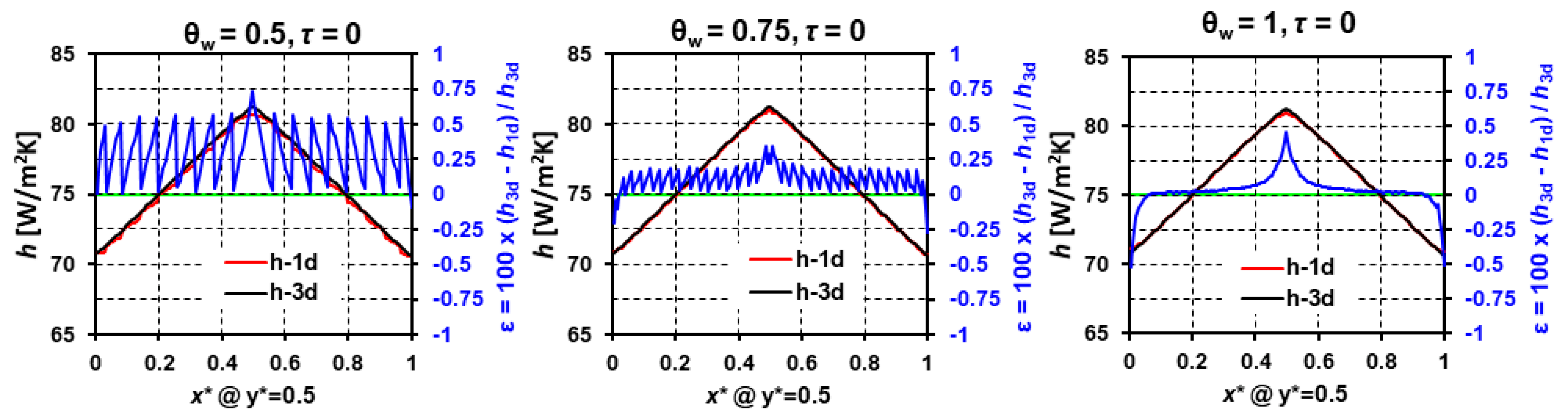
Consider Case I of a single jet for Re = 20,000 at
.
Figure 9a presents the
and
deviations for the three wall temperature tracking methods. For the shortest time duration tracking, i.e.,
, we observed noise in
and
difference data, which is attributed to spatio-temporal resolution. For higher
cases, the
and
deviations show a fixed trend where maximum deviation was observed at the jet stagnation and that
was consistently higher than
, except for the edges of the solid. This is again expected for a stagnation zone. The effect of
choice did not make much difference in the
and
deviations in Case I.
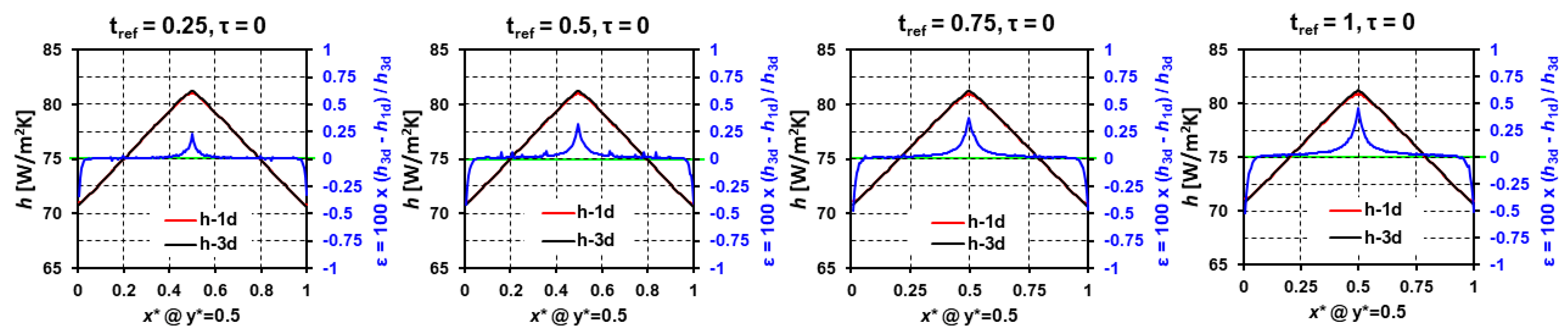
Figure 10b shows the local
and
deviations where the edge effects can be seen clearly, along with the stagnation region’s deviation, where
.
Figure 10 shows the
and
deviations along two lines y* = 0.375 and 0.5, as well as local deviations for Case II. The y* = 0.375 line showed maximum deviations at the low heat transfer regions where
was significantly higher than
, as observed for the
case presented earlier. The effect of
on resultant deviations in
and
can be seen where higher wall temperature tracking led to increasing deviations between
and
Hence, it is recommended that transient experiments be designed in a way that the wall temperature to be tracked is smaller, e.g.,
. The high heat transfer line, on the other hand, had
for all three
with
showing stronger fluctuations in deviation, which is attributed to grid resolution and time steps. It can be concluded that for high heat transfer zones,
does not have a significant effect on the deviations and that overall
by ~1%. The above trend for the high heat transfer line was also observed by [
16,
17]. The local deviations in
and
as shown in
Figure 10b demonstrate the above effect of
on the errors. Such a contour was also shown by Brack et al. [
16] for a theoretical distribution of
h representative of typical array jet impingement, where one jet at the center corresponding to the stagnation and the surrounding four were essentially the low heat transfer zones.
For Case III, the
and
deviations were smaller in general, and the effect of
was also reduced when compared to Case II. It can be deduced from the six sub-plots in
Figure 11a that there exists a trade-off between the low heat transfer and high heat transfer zones. It still appears to be a suitable strategy to track
in order to keep the low heat transfer zones with lower deviations since those zones exhibit significant deviations, as observed in other cases, and the high heat transfer zones have lower deviations (~1%). From the contour (
Figure 11b), it becomes increasingly clear that the
effect gets flipped for high and low heat transfer zones as we move from lower to higher values of
From an overall globally averaged deviations perspective,
is a better choice of reference temperature tracking where
is consistently higher than
with deviations within 4%. We did not track,
because of degrading spatial resolution in the context of local
h and time step marching (dt). From the liquid crystal thermography uncertainty point of view,
is recommended since it corresponds to lower uncertainties and that either direction of wall temperature (
) tracking would lead to higher uncertainties [
21].
However, from a theoretical perspective, one can always go for to analyze the further effects of this parameter on and deviations.
4.3. Method C: and Deviations at a Fixed ,
Note that so far, we have been analyzing a “global” wall temperature tracking method, where all pixels were tracked to the same wall temperature. This case is representative of typical transient liquid crystal thermography experiments where liquid crystals change color at a certain temperature band, and usually, a certain wall temperature corresponding to a particular color content and/or Hue value is considered as a reference temperature. Note that in such methods, the time taken to reach a particular fixed reference wall temperature may vary significantly depending upon the “true” h distributions. This may lead to significant uncertainty in h, as well as three-dimensional heat diffusion effects becoming prominent at longer time instances, particularly in the low heat transfer zones.
In Method C, the maximum temperature attained by each pixel () is determined, and the reference wall temperature that was tracked for each pixel was a function of , according to . In this method, each pixel is tracked to its own unique temperature, and such a method can be adopted in transient infrared thermography experiments where the time history of each pixel’s temperature is measured.
Figure 12 shows the
and
deviations for single jet configuration (Case I) for Re = 20,000 and τ = 0 for three values of
The first case (
exhibited effects of spatio-temporal resolution issues, with
. The
and
deviations tend to reduce in the wall jet region with increasing
while stagnation region deviations increased and converged to a sharp peak for
case. Note that these deviations are still very small and can be safely neglected. However, such a practice cannot be generalized for other singe jet studies, and each case should be evaluated exclusively since
and
deviations also depend upon the
true h(x,y).
Figure 13 shows the
effect where the
true h distribution and spatio-temporal resolution allowed coverage of
. For the low heat transfer line, clearly, the smaller value of
had significantly lower
and
deviations compared to
. Note that on the low heat transfer line, mostly
was higher than
, except for the relatively higher heat transfer zones (still on low heat transfer line y* = 0.375); however, those deviations can be ignored compared to that of the former. A reverse trend could be observed on the high heat transfer line (y* = 0.5), where
with larger deviations around the stagnation region. On high heat transfer line as well, a choice of smaller
would yield low values of deviations between
and
. Hence a best-case scenario for case study # 2 is a choice of
where deviations between
and
would be
However, a separate study on uncertainty analysis is recommended for such choices of short-duration transient experiments.
Figure 14 shows the
and
deviations for Case III with effects of
It can be observed that the deviations are random in nature, with major trends similar to those observed in Cases I and II. The contour of
and
deviations provide valuable information at both local and global levels. Overall,
and
appears to be balanced choices to keep the deviations at both stagnation and low heat transfer zones at low levels, in this case,
It is recommended that experimental studies involving transient infrared thermography perform the sensitivity analysis of
on ε, since this is a case-dependent result.
4.4. Method D: and Deviations at a Fixed ,
Methods C and D are similar in the way that each pixel’s wall temperature tracking is different. In Method D, each pixel is tracked up to a certain time instance in a transient experiment, which leads to different wall temperatures being tracked. Again, this method as well can only be employed in transient infrared thermography experiments or transient experiments employing wide band liquid crystals.
Figure 15 shows the
and
deviations for Case I where the effect of
is presented. The underlying trends observed in Methods A-C still hold true in this method as well, where shorter time duration-based wall temperature tracking yields lower deviations in
and
Overall, the wall jet region deviations were nearly zero, with stagnation point deviation increasing monotonically with increasing
; however, the maximum percentage deviation was still below 0.25%, which can be safely neglected in this particular case.
Figure 16 shows the deviations on low and high heat transfer lines for the Case II theoretical array jet impingement distribution. The trends of
and
deviations flip for the low and high heat transfer lines. At the stagnation zones,
while for the line passing through the low heat transfer zones, the
, where the low heat transfer line deviations were significantly larger than that of the high heat transfer line. Further, with increasing time matrix values, the deviations tend to increase for both the high and low heat transfer lines. The worst-case scenario for the deviations was the highest
where the deviations were between −30% to +5%. Hence, on a direct comparison between Cases I and II, one can clearly see the effect of large gradients in the
true heat transfer coefficient on the
and
deviations.
Figure 17 shows the
and
deviations for Case III of typical experimentally obtained distribution of
h. The overall trends observed for the high and low heat transfer lines for Case II hold true here as well, with deviations increasing with increasing time instances to be tracked. Further, the deviations at the jet stagnation point and in its close vicinity were found to be low only because of the nature of the experimentally obtained
h distribution as the local gradients in
h right underneath a jet was low. It appears that the
and
deviations correlate with the local gradients in the
h distribution as well. The above point is elucidated by the following contour of
and
deviations for Case III (
Figure 18).
The local of and deviations at the stagnation and at the low heat transfer zones between adjacent jets increased with increased . Further, the local deviations depend upon the local gradient in true heat transfer coefficient distribution. In this particular case of experimentally obtained h, the gradient in h at the jet stagnation was low, which resulted in overall lower deviations, which is different from what we observed for Case II. It is recommended that experimentally obtained h from 1-D semi-infinite conduction modeling should be re-evaluated for their discrepancies in obtained h in reference to the actual one. Such an evaluation would provide valuable information to the cooling designers as well as experimentalists to make better decisions on cooling designs and the design of experiments (DOE), respectively.


