Article

Leakage Analysis and Hazardous Boundary Determination of Buried Gas Pipeline Considering Underground Adjacent Confined Space

1
Gas Technology Institute of Petrochina Kunlun Gas Co., Ltd., Harbin 150000, China
2
School of Petroleum Engineering, Northeast Petroleum University, Daqing 163318, China
*
Author to whom correspondence should be addressed.
Energies 2022, 15(18), 6859; https://doi.org/10.3390/en15186859
Submission received: 24 August 2022 / Revised: 3 September 2022 / Accepted: 7 September 2022 / Published: 19 September 2022

Abstract

:
Urban underground construction projects are intertwined vertically and horizontally, and adjacent confined spaces such as water supply and drainage pipelines, side ditches and underground canals may exist near buried gas pipelines. Once the buried gas pipeline leaks, the gas will diffuse into the confined space through the soil and even enter the residential room by the confined space, which brings serious potential safety hazards. In this paper, the underground adjacent confined space hazardous boundary (HB) of underground gas pipeline leakage was defined, the distribution properties of gas leakage diffusion flow field were analyzed by numerical simulation and the distribution law of gas entering the confined space was studied. Using the least-squares method and multiple regression theory, the gas concentration prediction model in the adjacent confined space of buried gas pipeline leakage was established, the HB calculation model was further deduced, and the HB drawing board was drawn. The results showed that in the initial stages, the internal and external pressure and velocity distribution of the pipeline near the leakage hole were unstable, reaching a stable state after 60 s, and then the reverse flow occurred in the pipeline downstream of the leak hole. Reducing the minimum construction distance between the buried gas pipeline and the confined space improved the gas distribution concentration in the confined space. When the minimum construction distance increased from 3 m to 9 m, the gas concentration distribution decreased from 90.21% to 0.88%. Meanwhile, increasing the pipeline pressure and leakage diameter enhanced the gas concentration distribution in the confined space. The HB calculation model and HB drawing board realize the rapid determination of the HB between buried gas pipeline and confined space and offer a more reasonable basis for the design of gas pipeline safe distance in urban underground engineering construction.

1. Introduction

With the quick development of the gas industry and the acceleration of pipe network construction, gas supply capacity is continuously enhanced, and urban gas pipelines have become the energy main artery of national economic development. Common gases include natural gas, liquefied petroleum gas and coke oven gas. Natural gas gradually occupies a dominant position due to its large reserves and clean combustion. More than 90% of natural gas reserves exist in deep-sea clay or muddy sediments in the form of natural gas hydrate (NGH). The NGH reserves are twice the total reserves of proven oil, coal and natural gas, and 50 times the reserves of conventional natural gas, and can be used by humans for one thousand years [1,2]. At the same time, natural gas combustion can reduce the emission of the greenhouse gas carbon dioxide. The average hydrogen–carbon ratios of timber, coal, oil and gas are 0.1, 0.5, 2.0 and 4.0, respectively [3].
The gas has the advantages of good fluidity, low density and strong compressibility. Compared with other methods, pipelines are considered to be the safest and most economical mode of gas transportation [4]. Currently, buried natural gas pipeline networks are the most common mode of gas transmission [5]. However, great attention must be paid to buried gas pipelines because they carry flammable and explosive gases. Compared with the above-ground pipelines, the living environment of buried gas pipelines is harsh and hidden, so leakage accidents are frequent and difficult to detect, which brings serious hidden dangers to the surrounding soil and building areas. Moreover, the main component of natural gas is the greenhouse gas methane, which will affect the atmospheric environment after the leakage of buried pipelines [6,7]. Major gas explosion accidents in recent years have attracted the attention of the national government and all sectors of society. The safety of pipeline networks has affected the development of cities and social economy [8,9,10]. To avoid any gas pipeline accidents, to avoid a series of negative effects such as casualties, property losses and gas supply interruption caused by the accident, and to ensure the smooth and safe operation of gas pipeline networks are the goals pursued by all gas enterprises and even the country. Therefore, the gas leakage diffusion properties and danger analysis of damaged and failed natural gas pipelines are of great significance for gas leakage detection and secondary explosion accident reduction.
Theoretical analysis, experimental measurements and numerical simulation are important technical means to solve complex fluid flow. The test and numerical calculated results are intuitive and clear, which are the main way to study the gas diffusion law of gas pipeline leakage at present. Wakoh and Hirano put forward the prediction model of gas leakage concentration and carried out experimental measurements with combustible gas propane to verify the accuracy of the prediction model in calculating the leakage position, leakage time and leakage volume [11]. Houssin-Agbomson et al. used the experimental method to study the high-pressure gas-transmission pipelines’ accidental leakage conditions with the leakage diameter of 12 mm, and analyzed the influence of different factors on the concentration distribution of gas in the soil by changing the gas characteristics, pipeline operating pressure and soil properties, so as to realize the accurate assessment of leakage accident risk [12]. Pokhrel et al. carried out experimental research and theoretical analysis on the diffusion of gas in three porous media, measured the value of the gas diffusion coefficient, developed a new empirical model using the experimental results and compared and analyzed the calculated values with the existing empirical model [13]. In the aspect of numerical simulation, Wilkening and Baraldi used a numerical simulation method to compare and analyze the gas diffusion process of small holes leaked in high-pressure hydrogen pipelines and gas pipelines [14]. Bezaapour et al. regarded gas as real gas; considered the soil anisotropy, stratification, and soil water content of each layer and soil slope; and studied the influence of different factors on the gas dispersion process by transient simulation [15]. Bu et al. divided the ground conditions into hardened surface ground, unhardened surface ground and semihardened surface ground; considered the influence of the soil properties of the pipeline’s living environment on the gas leakage and dispersion process; established the calculation equations of the buried gas pipeline leak rate, gas invasion distance and the early warning boundary; and formed a systematic calculation method [16,17].
In addition to the experimental and numerical simulation methods, Pontiggia et al. developed a technology to import the terrain database into the CFD simulation tool, which allows for a simple but very detailed analysis of all building geometries in the real urban environment, so as to realize the rapid assessment of the gas leakage area risk degree [18]. Lovreglio et al. proposed a dynamic calculation model considering gas diffusion and personnel evacuation at the same time; discussed the difference between the results obtained by the existing static method and dynamic method; considered the movement of personnel with different complexities; and effectively improved the accuracy of the gas toxicity disaster risk assessment [10]. Badida and Sklavounos obtained the possible results of accidental gas release through fault tree analysis and determined the safety distance around the gas pipeline leakage accident [8,19].
A large number of existing research results have analyzed the gas diffusion characteristics after the pipeline leakage. However, due to the interweaving of urban underground engineering construction, there may be water supply and drainage pipelines, side ditches, culverts and other adjacent confined spaces near the buried gas pipeline at the same time. After the leakage, the gas diffuses into the confined space through the soil, and even enters the room through the confined space, resulting in serious potential safety hazards. On 4 July 2017, a buried gas pipeline leaked in Songyuan City, Jilin Province, China, and the gas entered the complex building of the municipal hospital through the sewer pipeline, leading to 5 deaths and 89 injuries [20]. Currently, research on gas entering the underground adjacent confined space through soil after the leakage of a buried pipeline has not been involved.
This paper defines the hazardous boundary (HB) of underground adjacent confined space of buried gas pipeline leakage and studies the diffusion process of leaked gas from a buried pipeline into a confined space through soil by combining transient and steady-state numerical simulation. The transient simulation method was used to analyze the basic properties of flow field distribution in the pipeline, leakage hole and soil after the buried pipeline leaked, and the concentration distribution process state of gas entering the confined space was studied. The most dangerous state of gas distribution in the confined space was studied by the steady-state numerical simulation method, and the limit distribution concentration was determined. Based on the least-squares method and multiple regression theory, the computational model between the gas concentration distribution and various factors in the confined space was established. The mathematical calculation software MATLAB was used to calculate and solve, and the gas concentration prediction model in the confined space was obtained. Based on the principle of heavy risk and the prediction model of gas concentration in a confined space, the underground adjacent confined space HB computational model of buried gas pipeline leakage was deduced and established. This study provides a more scientific and reasonable basis for the safety distance design of buried pipeline construction in urban underground engineering.

2. Methods

2.1. Physical Model

Ebrahimi-Moghadam et al.’s research showed that the two-dimensional model cannot consider three-directional resistance of the gas dispersion in the soil, increasing the calculation error [21,22]. Therefore, the three-dimensional physical model of the dispersion of leaked gas from a buried pipeline in soil was established. In order to study the flow field distribution characteristics in the pipeline, leakage hole and soil after the leakage of a buried pipeline, pipeline modeling was taken into account. The model took cuboid soil (11.5, 4, 2 m); the pipeline ran through it along the x-axis direction, and the wall thickness of the pipeline was 5 mm. The Cartesian coordinate system was established with the axis of the pipeline where the leaked hole was located as the coordinate origin, as shown in Figure 1.
In addition to buried gas pipelines, urban underground engineering construction is often accompanied by confined spaces such as water supply and drainage pipelines, side ditches and culverts. After the buried gas pipeline leakage, the gas diffuses into the confined space and even enters the room through the confined space, bringing serious potential safety hazards. The distance between the underground confined space and the leaked hole of the gas pipeline affects the gas concentration distribution in the soil around the confined space, which is bound to affect the distribution concentration of the gas entering the confined space. Based on the principle of heavy risk, the minimum construction distance between the buried gas pipeline and the confined space was the distance L between the pipeline leakage hole and the central point of the confined space damaged position, which was the distance with the greatest danger on the confined space after the gas leakage. According to the water supply and drainage design manual [23], the buried depth of the upper surface of the confined space of the underground culvert from the ground was 0.5 m, and the horizontal dimension of the rectangular section was not less than 0.5 m, and the vertical dimension was not less than 0.6 m. In this study, the rectangular size of confined space section was set to 0.8 × 0.6 m and leakage radius size was 0.25 m (minimum cross-section horizontal-size circular crack). Since the construction distance L between the buried pipeline and the confined space was involved, the physical model size in the Y direction was increased to 11.5 m, as shown in Figure 1.

2.2. Mathematical Model

2.2.1. Basic Conservation Equation

In this paper, the gas leaking and diffusion characteristics of damaged and failed urban buried medium-pressure gas pipelines were studied. When the ambient temperature is not too low and the pressure is not too high, the flow process of gas can be regarded as the ideal gas adiabatic flow [24,25]. After the leakage, the gas is ejected through the leakage hole of the pipeline and diffuses in the soil. Compared with gas flow in the atmosphere, the flow and dispersion process of gas in the soil is affected by soil porous media resistance and porosity. The soil porosity needs to be added in the continuity equation, motion equation and energy equation, and the soil resistance source term composed of viscous resistance and inertial resistance needs to be added to the motion equation [26,27,28].
t ( ρ ϒ ) + ( ρ v ) = 0
ϒ ρ v t + ρ ϒ 2 ( v ) v = p + μ ϒ 2 v + ϒ ρ g + S i
x i ( ρ s E s ) + x i [ v ( ρ s E s + p ) ] = x j [ k e f f T x j + v ( τ i j ¯ ¯ ) e f f ]
where t is leakage time (s), ρ is density (kg/m3), ϒ is soil porosity, v is velocity vector (m/s), p is absolute pressure (Pa), μ is the dynamic viscosity of gas (Pa·s), g is the acceleration of gravity (m/s2), S i is the soil resistance source term, x is displacement (m), E is total energy (J), k is conductivity factor (W/mK), T is temperature (K), τ ¯ ¯ is second order stress tensor (Pa), and the subscript “ e f f ” is effective.
The gas flow of buried gas pipeline leakage in soil is influenced by the soil porous medium resistance, including viscous resistance and inertial resistance. Assuming that the soil is isotropic porous medium, the source term ( S i ) of the dynamic equation composed of soil viscous resistance and inertial resistance can be expressed as [29,30]:
S i = ( μ α v i + C 2 ρ 2 | v | v i )
The Ergun equation can determine the soil resistance coefficients, as shown in Equation (5).
| Δ p | Δ L = 150 μ v D p 2 ( 1 ϒ ) 2 ϒ 3 + 1.75 ρ v 2 D p ( 1 ϒ ) ϒ 3
The viscous resistance ( 1 / α ) and inertial resistance ( C 2 ) can be calculated by comparing Equations (4) and (5), as shown in Equations (6) and (7).
1 α = 150 D p 2 ( 1 ϒ ) 2 ϒ 3
C 2 = 3.5 D p ( 1 ϒ ) ϒ 3
where Δ p is the flow direction pressure drop (Pa), Δ L is the length in the pressure gradient direction (m), and D p is the soil mean diameter (mm).

2.2.2. Component Transport Equation

After the pipeline leakage, the flow and dispersion of gas in the soil involve the mixing of gas components and air. Since there are more than two kinds of gases, the component transport equation needs to be considered. The specific form of component transport equation is as follows [29,30]:
ϒ t ( ρ ω ) + ( ρ ω v ) = ( ρ D ω )
where ω is the gas component mass fraction (%) and D is the gas diffusion coefficient.

2.2.3. Gas-State Equation

According to design code of city gas engineering [31], when the pipeline pressure is less than or equal to 1.2 MPa, the gas compression factor is 1. After the leakage of the buried medium pressure gas pipeline, the gas flow in the pipeline and soil is the ideal gas adiabatic flow,, which meets the ideal gas-state equation and the mixed gas viscosity equation [15,32]:
p = ρ R T M
μ m i x = i = 1 n μ i 1 + j i ϕ i j y i / y j
ϕ i j = { 1 + ( μ i / μ j ) 1 2 ( M j / M i ) 1 4 } 2 2 2 ( 1 + M i / M j )
where ρ is gas density (kg/m3), R is gas constant (J/kg⋅K), μ m i x is mixed gas viscosity (Pa⋅s), y is mole fraction (%), M is molecular weight (kg/mol).

2.2.4. Turbulence Model

The Reynolds number of gas flow in the pipeline is high, and the flow is obviously turbulent. The κ ε standard turbulence model is used for calculation. The κ ε standard model is two-equations model, which introduces the turbulent dissipation rate ε equation based on the turbulent kinetic energy κ equation. The model supposes that the flow is complete turbulence and ignores the influence of molecular viscosity. The specific form of the κ ε standard model is as follows [33,34,35]:
t ( ρ κ ) + ( ρ κ u ) = [ ( μ + μ t σ κ ) κ ] + G κ + G b + Y M ρ ε
t ( ρ ε ) + ( ρ ε u ) = [ ( μ + μ t σ ε ) ε ] + ε κ ( C ε 1 G κ C ε 2 ρ ε )
where κ is turbulence kinetic energy (J/kg), ε is turbulence dissipation rate (J/kgs), G κ is turbulence kinetic energy generation, G b is turbulence kinetic energy generation, Y M is the influence of fluctuating expansion on total dissipation rate in compressible turbulence, μ is viscosity (Pa·s) and μ t is turbulent viscosity. C ε 1 , C ε 2 , σ κ , σ ε are empirical constants with values of 1.45, 1.90, 1.0 and 1.25, respectively [36,37,38].

2.3. Scenario Design

There are many factors affecting the leakage and diffusion of leaked gas from buried gas pipelines in soil, among which the important factors are pipeline pressure, leakage diameter, pipeline buried depth and soil type. The pipeline diameter has little effect on the flow process of gas [29,30]. According to design code of city gas engineering [31], the buried depth of pipeline is 0.3–1.5 m. Based on the principle of heavy risk and considering the location of confined space, the buried depth of pipeline was set as 1.5 m. The common soil types were sandy, loam and clay, the resistance of gas diffusion in the three types of soil gradually increased, and the loam was selected for research. Based on the above analysis, the main influencing factors studied were pipeline pressure (p), leakage diameter (d) and the minimum construction distance (L) between buried gas pipeline and confined space. The pressure of urban medium-pressure buried gas pipeline was 0.2–0.4 MPa, the leakage diameter range was 20–60 mm [29,30], and the minimum construction distances were 3 m, 5 m, 7 m and 9 m. The concrete working condition settings were shown in Table 1.
Transient numerical simulation calculation was carried out using Case 10 in Table 1, in which the confined space was closest to the leak hole of the buried gas pipeline and the process state of gas entering the confined space was analyzed. Through the study of pressure, velocity, streamline and gas concentration distribution in the pipe, leakage hole and soil after the leakage, the leakage and diffusion characteristics of gas in soil were analyzed. After the pipeline leakage, the damaged area was the public part of the pipeline and soil at the leakage hole. In order to study the parameter changes inside the pipeline near the damaged area and in the soil above, the pipeline internal monitoring points 1 (0, 0, 0 m) and 2 (0, 0, 0.050 m) of the leakage hole and the monitoring points 3 (0, 0, 0.055 m) and 4 (0, 0, 0.105 m) in the soil were set to monitor the pressure and velocity, the effect of soil resistance on the leakage process in the damaged area was analyzed. The monitoring point 5 was used to monitor the concentration distribution change of gas entering the confined space, as shown in Figure 2.
The leakage accident of the buried gas pipeline was not found in time, and the gas diffused in the soil and confined space until it reached a stable state. The steady-state numerical simulation calculation was carried out under all working conditions in Table 1 to study the influence of pipeline pressure, leakage size and the minimum construction distance between buried pipeline and confined space on the gas concentration distribution in confined space, and the safe construction distance was determined according to the gas concentration distribution.

2.4. Grid Generation and Numerical Method

Grid generation is a discretization process that divides the fluid calculation domain into finite small elements, which has a serious impact on the accuracy and speed of calculation results. Reducing the number of grids may increase the calculation error or lead to the divergence of calculation results, while too many grids will increase the quantity of calculations and calculation time. To ensure the calculation accuracy and reduce the calculation time, the hexahedral structured grid was divided into four grid levels to test the grid independence [39,40]. Taking the vertical line of the leakage hole as the center, the cylindrical area with a radius of 0.5 m was divided by interface, and the area near the buried pipeline leakage hole was locally densified.
In this paper, based on the FVM (finite volume method) of Fluent software, the diffusion of leakage gas from buried pipelines in soil was studied by combining transient and steady-state numerical simulation, and the distribution of gas diffused into confined space through soil was considered. For the coupling solution of velocity and pressure in N-S equation, PISO algorithm and SIMPLE algorithm were used for transient and steady-state condition simulation, respectively, and the pressure was modified twice [22,41]. Since the leakage and diffusion process of gas in soil after the failure of buried gas pipeline involved the changes of energy, components and turbulent flow pattern, it was also necessary to solve the energy equation and set the mixed components of gas and air in the component transport equation. In order to improve the accuracy of numerical calculation, the convection term adopts the second-order upwind discrete scheme, and the turbulence correction equation adopts the κ ε standard model. The time step of transient simulation was set to 0.1 s, the number of time steps was 108,000, and the maximum number of iterations was 100. Based on the set numerical simulation scheme, the diffusion characteristics of gas in soil within 3 h after the leakage of buried gas pipeline were simulated. Because the density of gas was smaller than that of air, gravity and buoyancy had a great impact on the diffusion process. Therefore, considering the influence of gravity and total buoyancy, the gas component was regarded as methane with a concentration of 100% [42]. In order to improve the presentation effect of cloud images of numerical simulation results, the calculation results were imported into Tecplot software for postprocessing and analysis, and the monitoring point results were imported into Origin professional data processing software for processing.

2.5. Boundary Conditions and Initial Conditions

The modeling of pipeline was considered in this study, so the pipe inlet was set as pressure inlet and the pipe outlet was pressure outlet. The boundary around the soil and the bottom end were connected with the soil, and the upper end was connected with the atmosphere through the unhardened ground, so they were all set as the pressure outlet boundary. The confined space was an enclosed space, which was set with wall boundary. Compared with the overall model structure, the size of the leakage hole of the buried pipeline was smaller, and the global grid division of the overall structure increased the grid distortion at the leakage hole. Therefore, a cylindrical area with a radius of 0.5m in the longitudinal direction was established with the vertical line where the center of the leakage hole was located as the center, which was divided by the interface, and the internal grid was locally densified. Due to the large size of the leakage location in the confined space, there was no need for local mesh encryption. The specific boundary type definitions were shown in Table 2.
Before the gas pipeline leakage, the pipeline was filled with gas, and the pressure was the pipeline operating pressure. The pores of soil porous media were filled with air, and the pressure was equal to the atmospheric pressure. After the boundary conditions were defined and the fluid calculation domain was initialized, the Patch command was used to repair the gas composition, pressure distribution and other relevant parameters of the pipeline and soil calculation domain, respectively, to ensure the accuracy of the numerical calculation results.

3. Results and Discussion

3.1. Grid Independence

Grid independence was verified by taking the gas leakage rate at the leak hole of buried pipeline as the judgment standard. It was divided into four grid levels, with the quantities of 514,784, 1,133,662, 1,502,339 and 1,887,451, respectively. The calculation errors of the gas leakage rate at the four grid levels were 7.66%, 2.39% and 0.76%, respectively, as shown in Table 3. To ensure the accuracy of the calculation results and shorten the calculation time, the 1,502,339 grid number was chosen for the numerical simulation calculation, to reduce the calculation error caused by the grid number to less than 1%.

3.2. Model Validation

In order to ensure the reliability of the numerical calculation method, Okamoto et al.’s experimental results were used to verify the reliability of the numerical simulation results [32]. According to the experimental model, the rectangular soil physical model with the size of 10 × 10 × 2.9 m (X × Y × Z) was re-established, and the three-dimensional rectangular coordinate system was established, with the ground directly above the center of the leakage hole as the coordinate. According to the laying method of the experimental pit, the Z direction was composed of 5 cm asphalt, 15 cm crushed stone and 2.7 m sand from the ground down. The three types of buried media landfill areas were divided into three fluid domains, and the porous media parameters were set, respectively. The characteristic parameters of the three types of buried media are shown in Table 4. The numerical simulation settings were consistent with the experimental parameters, and the experimental gas was studied with 100% methane. The leakage hole was located at the center of the plane Z = −1.2 m below the ground. The pressure of the leakage hole was 0.2 kPa and the amount of leakage was 1150 (Ncc/min).
The experimental monitoring points Coordinate A (0.3, 0, −0.6m) and Coordinate B (1.1, 0, −1.6m) were used to monitor the concentration distribution of methane gas in soil. The numerical calculation results of gas concentration distribution at Coordinate A and Coordinate B were basically consistent with the experimental trend, with an average error of 6.05%, indicating the accuracy of the numerical method in this paper, as shown in Figure 3.

3.3. Analysis of Gas Leakage and Dispersiong Characteristics

In this study, the soil was considered as isotropic porous media, which was symmetrically distributed in the soil after gas leakage. In order to analyze the internal flow field distribution of the gas leakage pipeline, the Y = 0 plane flow field distribution was studied. At the beginning of the leakage of the buried gas pipeline, the distribution of flow fields such as pressure, velocity and streamline in soil changed sharply, and reached an equilibrium state after 100 s [29,30]. In order to study the variation of flow fields in the pipeline, leakage hole and soil of buried gas pipeline leakage at the initial time of leakage, Case 10 was used to analyze the change process of flow fields within 100 s of gas pipeline leakage.

3.3.1. Pressure Distribution

Once the buried gas pipeline leaked, the pressure at the internal monitoring point of the pipeline at the leakage hole and the monitoring point in the soil above displayed different trends with time, and reached an equilibrium state within 60 s. At the beginning of the leakage, the gas was rapidly ejected by the pressure difference inside and outside the pipeline, and the pressure at monitoring points 1 and 2 in the pipeline decreased rapidly. Since the upstream gas supply valve of the pipeline was not closed, the continuous supply of gas immediately rose to a stable state. Monitoring points 3 and 4 in the soil above the leak hole showed the opposite sudden enhanced trend, slightly decreased after reaching the peak pressure, and then reached an equilibrium state. The pressure of the monitoring point inside the pipeline near the leakage hole was low (Point 2), and the pressure of the monitoring point in the soil outside the pipeline near the leakage hole was high (Point 3). The pressure change inside the pipeline was small, and the pressure change in the external soil was large, as shown in Figure 4.
After the leakage, the gas inside the pipeline at the leakage hole ejected rapidly, resulting in a sudden decrease in the pressure at monitoring points 1 and 2. It was supplemented under the continuous supply of gas in the rear pipeline, and the pressure gradually rose to a stable state. The pressure at monitoring point 3 and monitoring point 4 in the soil was atmospheric pressure before the leakage. After the leakage, the pressure of the gas jet rose under the resistance of the soil, resulting in a sudden increase in the pressure at the monitoring point. With the continuous occurrence of leakage, the gas diffused through the soil to the surroundings, and the pressure gradually decreased to a stable state. When the pressure in the soil near the leakage hole reached the equilibrium state, the gas diffused outward in this state, which was not the steady-state equilibrium of the global pressure. The area near the leakage hole first reached the equilibrium state and diffused outward in this equilibrium state. The equilibrium area gradually expanded in a ring, and finally reached the steady-state equilibrium. During the flow process of gas leakage and dispersion, monitoring point 1 was located upstream of monitoring point 2, and the pressure was higher. Since monitoring point 3 was located at the center of the leakage orifice outside the pipeline, the pressure was large after the pipeline leaks. Monitoring point 4 was located 50 mm above the leakage orifice, which was more affected by soil porous media resistance, and the pressure was lower than that of monitoring point 3 at the leakage hole.
With the leak hole as the center, the pressure in the soil and pipeline presented a symmetrical distribution state. The pressure inside the pipeline and near the leakage hole was high, and the pressure from the leakage hole to the surrounding soil showed a sharp decrease trend. Close to the internal monitoring points 1 and 2 of the pipeline, after the leakage of the buried gas pipeline, the gas was rapidly ejected, resulting in a sudden decline in the internal pressure of the pipeline. With the continuous supply pressure of the gas at the gas supply end of the pipeline, it gradually rose and reached an equilibrium state after 60 s, as shown in Figure 5. The soil isotropic assumption made the pressure distribution in the soil present a symmetrical state. The broken part of the buried gas pipeline was the common section between the pipeline and soil. Soil resistance made the input and output pressure on each section of soil different. Taking the leakage hole as the center of the circle and diffusing into the external soil, the soil of each section played the role of decompression, resulting in a sharp decline in the pressure around the soil.

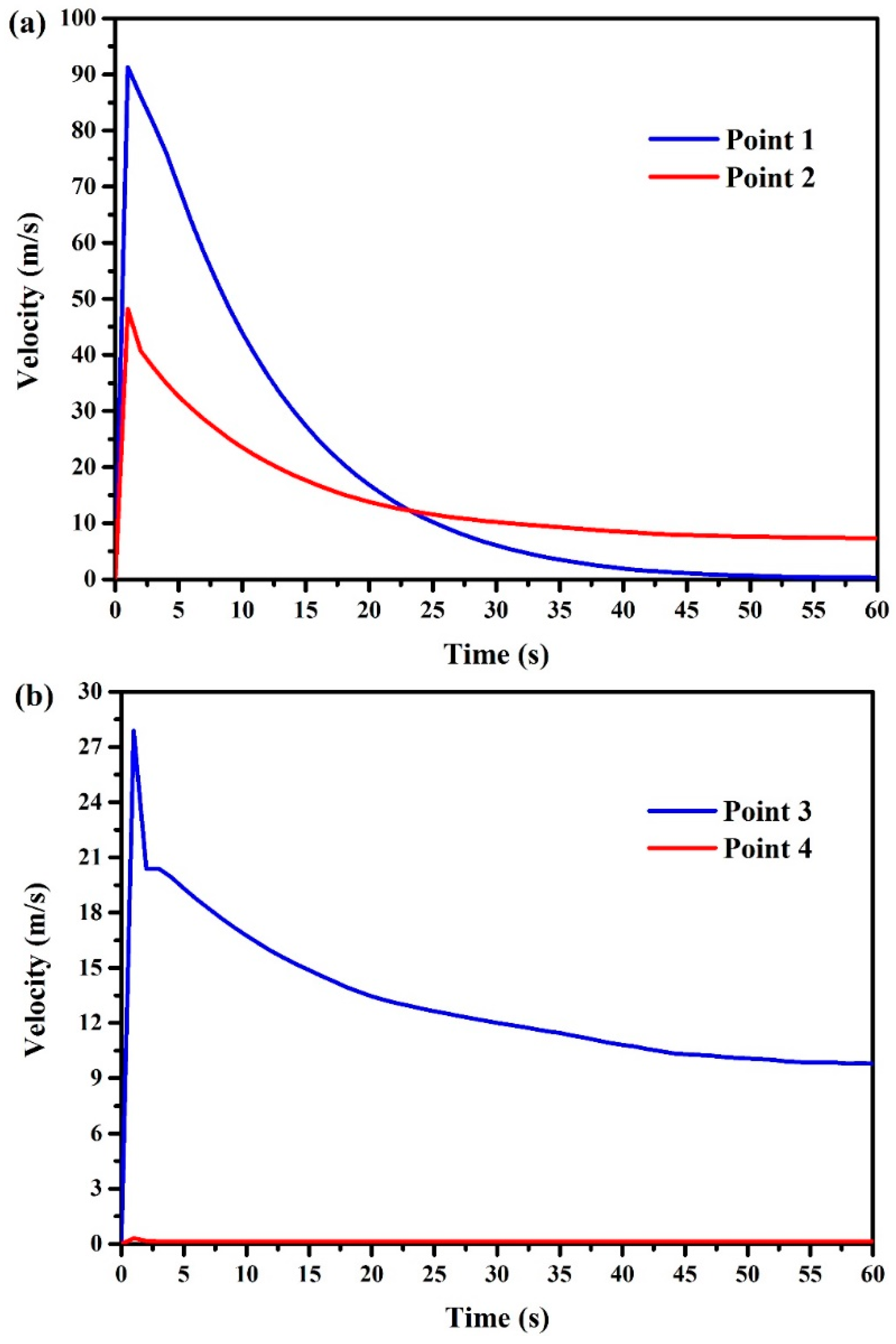
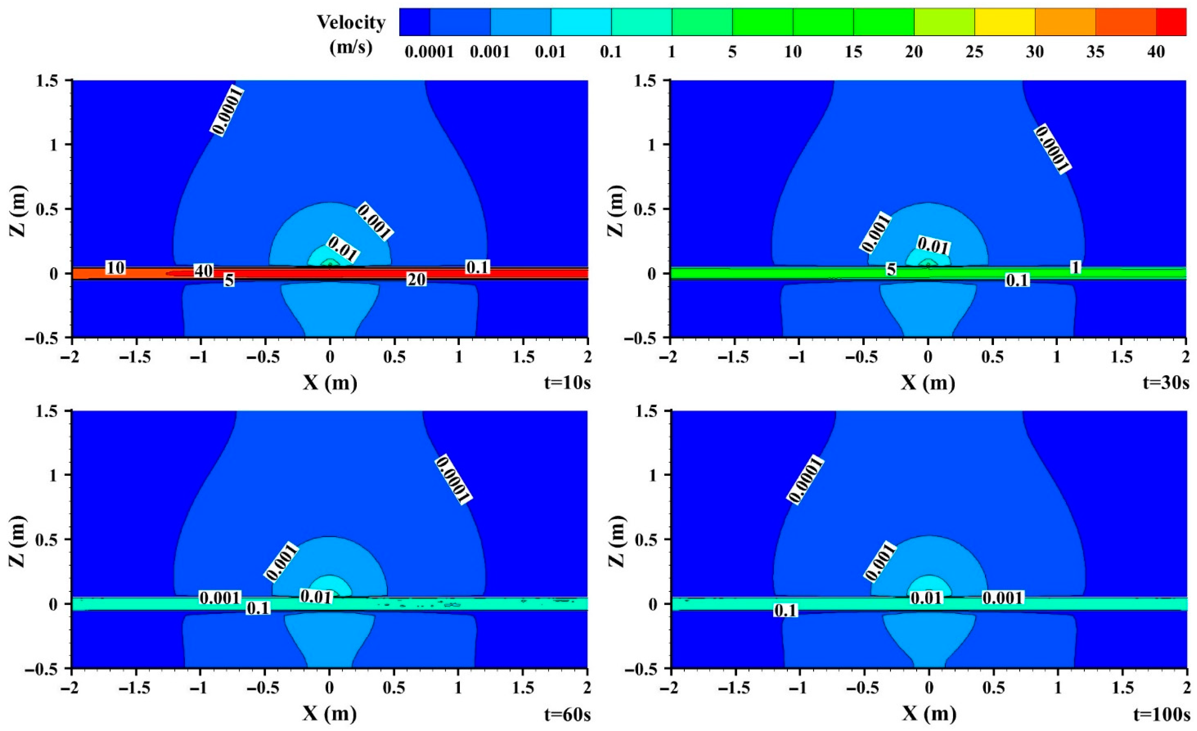
3.3.2. Velocity Distribution

After the pipeline leakage, the velocity at the monitoring points in the damaged area first increased sharply and then decreased gradually, and reached an equilibrium state after 60 s, as shown in Figure 6. When the leakage occurred, the gas in the pipeline was rapidly ejected from the leakage hole, and the gas in the pipeline flowed to the leakage hole to supplement. The pressure difference inside and outside the pipeline at the moment of leakage was the operating pressure of the pipeline, and the flow velocity was fast. According to the pressure change monitoring, the pressure in the damaged area outside the pipeline increased under the action of soil resistance after the leakage, and the pressure difference between inside and outside the pipeline near the leakage hole decreased, resulting in a gradual decrease in the velocity. When the pressure difference near the leakage hole reached the equilibrium state, the leakage velocity reached an equilibrium state, including the gas leakage velocity at monitoring point 2 at the leakage hole and the rear gas supply velocity at monitoring point 1. Due to the small leakage diameter, the gas supply velocity at the rear was significantly less than that at the leak hole. For monitoring point 3 above the leakage hole, the distribution of leakage velocity was similar to that of monitoring point 2, which was located on the inside and outside of the pipeline at the leak hole. Monitoring point 4 was further away from the leakage hole, more affected by soil porous media resistance, and the speed was significantly reduced.
Similar to the pressure distribution, with the leak hole as the center, the gas flow velocity in the soil was symmetrically distributed, and the velocity distribution from the leakage hole to the outside was significantly reduced. In the initial stage of leakage, the internal velocity distribution of the pipeline was large. With the occurrence of leakage, the velocity gradually decreased and reached a stable state after 60 s, as shown in Figure 7. At the beginning, due to the large pressure difference inside and outside the pipeline, the leakage velocity was fast, and the gas in the pipeline was rapidly replenished, and the flow rate was large. After leakage for a period of time, the leakage velocity decreased and gradually reached an equilibrium state, and the supply flow velocity inside the pipeline also showed the same trend. For buried gas pipelines, the soil porous media resistance reduced the flow velocity when the gas was ejected into the soil. With the increase in the resistance time of gas diffusion, the flow velocity gradually decreased, resulting in the gradual decrease in the outward velocity from the leakage hole.

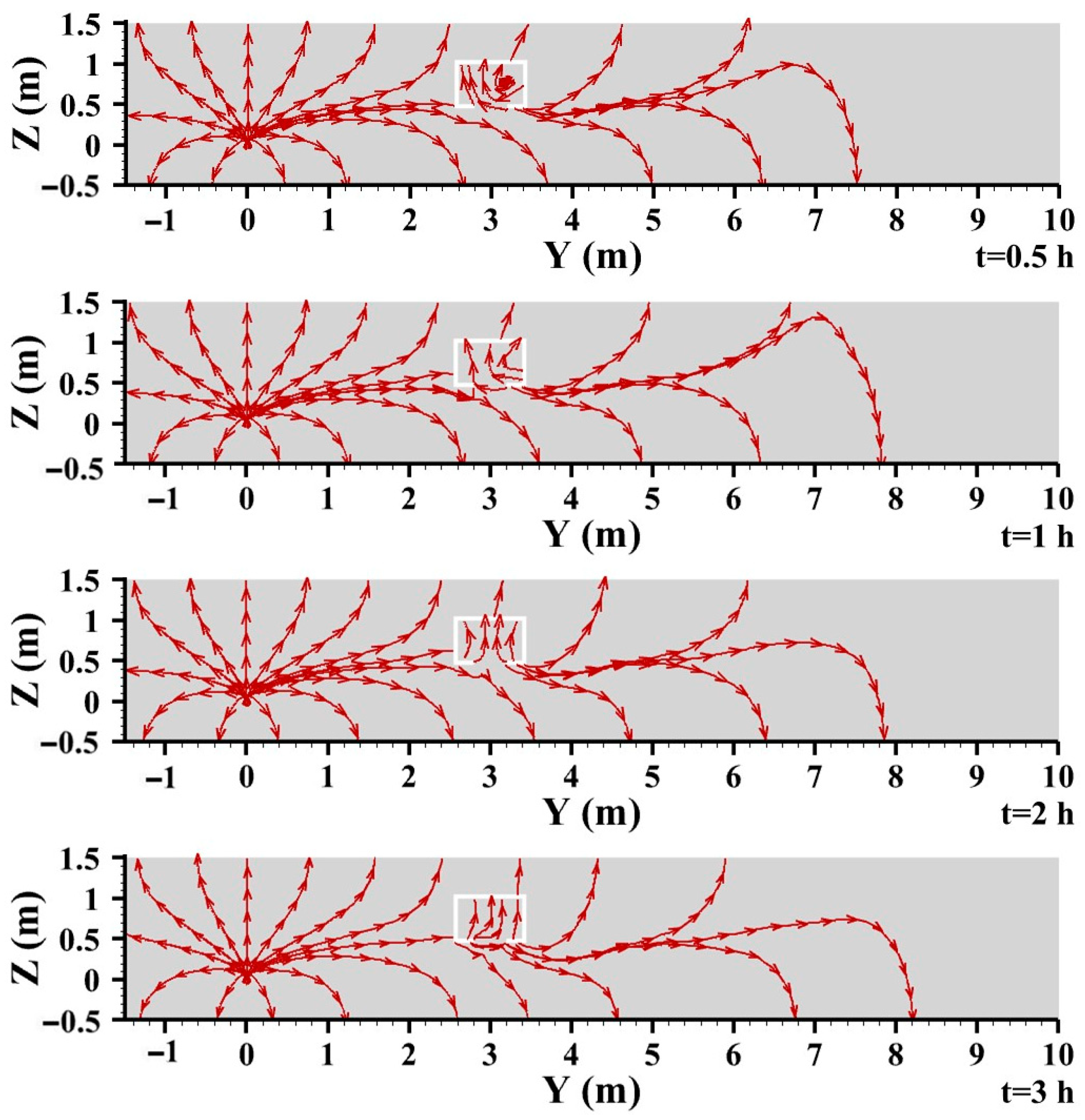
3.3.3. Streamline Distribution

Based on the assumption of soil isotropy, the gas leakage flow streamline presented a symmetrical distribution state. After gas leakage, the streamline distribution in the soil was basically unchanged, and the streamline distribution inside the pipeline changed greatly. At the beginning, the direction of air flow in the pipeline was from upstream to downstream, but the pipeline downstream of the leak hole appeared countercurrent after 60 s, as shown in Figure 8. At the initial stage of leakage, due to the fast leakage velocity, it needed the rapid replenishment of the upstream pipeline. As the leakage rate tended to be stable, the leakage rate decreased and the upstream gas supply velocity slowed down. At this time, the stable leakage was supplied by the upstream and downstream countercurrent of the pipeline, and the countercurrent phenomenon occurred in the leakage hole pipeline downstream.
In order to analyze the dispersion process of gas into confined space through soil after the buried pipeline leakage, the cloud diagram of X = 0 plane streamline distribution was analyzed. Since the gas cannot enter the confined space for the first time at the initial period of leakage, the research time was extended to 3 h, as shown in Figure 9. After the buried gas pipeline leakage, the gas diffused in the soil and entered the confined space through the damaged position of the confined space, accompanied by the outflow of gas inside the confined space. Leakage time had no influence on the streamline distribution of gas diffusion in soil but had a great influence on the streamline distribution in the confined space. A vortex was formed at the initial stage of gas diffusion into the confined space, and gradually disappeared with the extension of leakage time. The continuous entry of gas into the confined space led to the gradual increase in the internal pressure of the confined space, and part of the gas flowed out of the damaged position of the confined space and into the soil under the action of the pressure difference between the confined space and the soil. The gas diffused through the soil and gradually entered the confined space to mix with the internal air to produce an eddy current. With the continuous entry of the gas in the confined space, the concentration increased, the mixing degree with the air tended to be stable, the eddy current gradually disappeared, and finally the state of dynamic balance of gas inflow and outflow at the damaged position of the confined space reached.

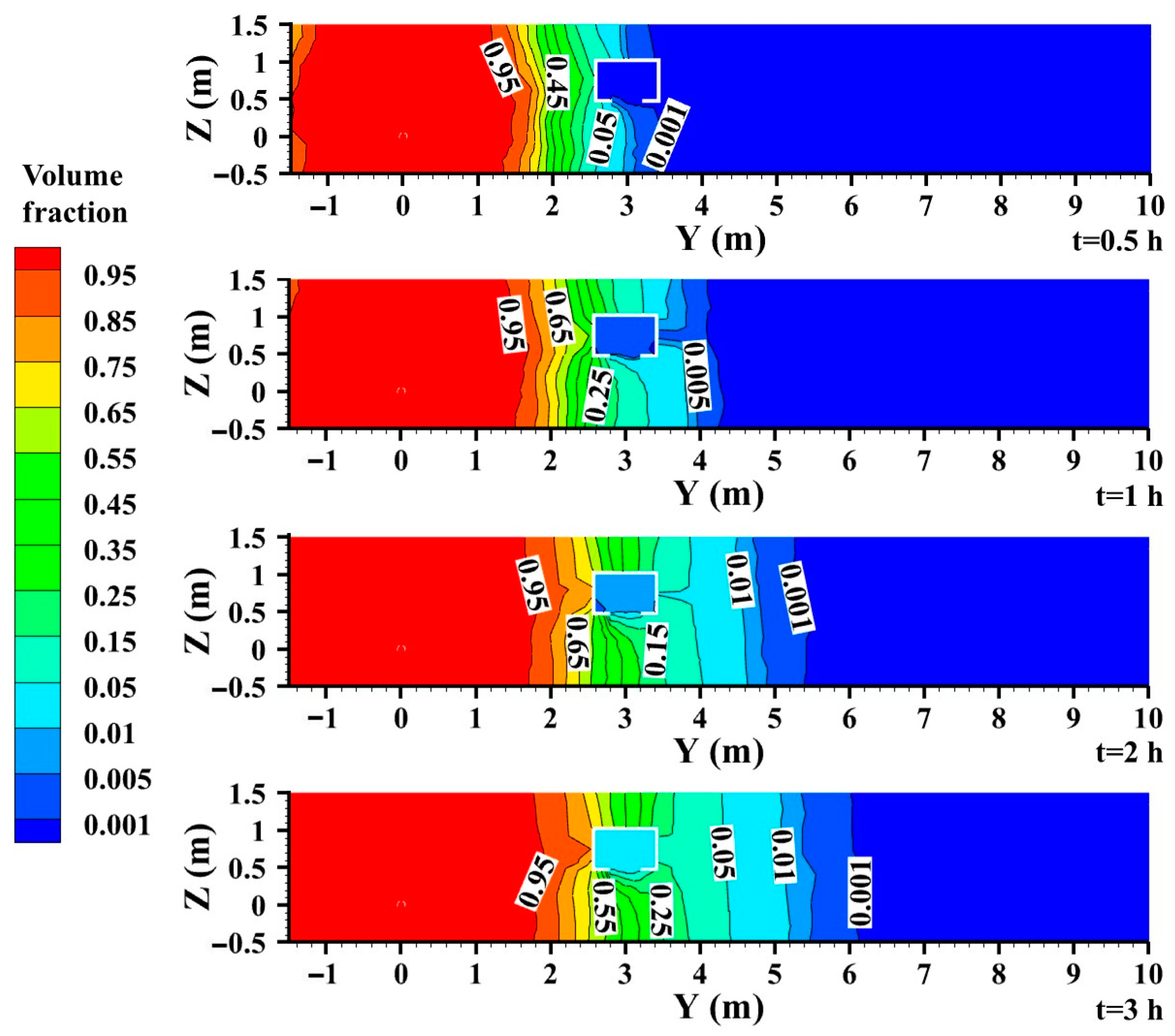
3.3.4. Gas Concentration Distribution

To study the transient process of leakage gas from the pipeline passing through the soil into the confined space, the x = 0 plane gas concentration distribution was analyzed, as shown in Figure 10. After the buried gas pipeline leakage, the gas entered the confined space through the soil. With the continuous leakage, the gas concentration in the confined space enhanced gradually. When the gas leakage time lasted from 0.5 h to 3 h, the average gas concentration on the x = 0 interface in the confined space was enhanced from 0.05% to 1.74%. After the buried pipeline leakage, the gas diffused in the soil. When the gas diffused to the damaged position of the confined space, the gas entered the confined space under the action of the concentration difference inside and outside the confined space. With the continuous occurrence of leakage, the gas concentration in the soil outside the damaged position of the confined space gradually increased, and the gas diffused into the confined space under the action of concentration difference, resulting in the gradual increase in gas concentration in the confined space. With the continuous diffusion and accumulation of gas into the confined space, the concentration reached the explosion range and brought serious potential safety hazards. In addition, some confined spaces, such as sewer pipes and drainage ditches, may be connected with the interior of residential buildings. Once the gas enters the space for human survival and activities through the confined space, it will pay a heavy price in the cases of explosion.
Figure 11 shows the change process of gas concentration distribution with leakage time at monitoring point 5 in the confined space. Since the confined space was far away from the leakage point, there was no gas distribution at 5 monitoring points at the leakage initial period. With the extension of the leakage time, the gas distribution gradually began at monitoring point 5, and then the concentration gradually increased, which was similar to the cloud diagram of gas concentration distribution in Figure 10. Due to the slow progress of the transient diffusion process of gas, in order to obtain the distribution state of gas in the confined space under the limit state, the steady-state simulation method was used to further study the hazardous boundary of the confined space.

3.4. Determination of Underground Adjacent Confined Space Hazardous Boundary

3.4.1. Definition for Hazardous Boundary of Underground Confined Space

There is no combustible gas leakage detection device in the underground confined space, and the diffusion of gas in the confined space is not easy to detect. In order to avoid a secondary explosion accident caused by gas leakage into the confined space, the diffusion concentration distribution of gas passing through the soil into the underground confined space was studied to determine the minimum safe construction distance between the buried gas pipeline and the underground adjacent confined space. The hazardous boundary (HB) of buried gas pipeline and underground confined space is defined as follows: When the distance L between the leakage hole of the buried gas pipeline and the center point of the underground confined space damaged position (the minimum construction distance between the buried gas pipeline and the confined space) is equal to the hazardous boundary (HB), the maximum concentration of the gas leakage into the confined space is equal to the lower explosive limit of the gas (5%VOL), and the distance L is the hazardous boundary (HB) of the confined space.
When the minimum construction distance L between the buried gas pipeline and the confined space is greater than the hazardous boundary, the gas concentration distribution in the confined space after the leakage accident is always less than the lower explosion limit, which is the safety reference distance of the buried gas pipeline construction project, as shown in Figure 12.

3.4.2. Analysis on Influencing Factors of Gas Concentration in Confined Space

Among the influencing factors, the pipeline operating pressure (p), leakage diameter (d) and the minimum construction distance (L) between the buried gas pipeline and the underground confined space were selected, and the steady-state numerical simulation calculation was carried out by using the working conditions in Table 1. According to the influence of various factors on the steady-state distribution concentration of gas in the confined space, the analysis and prediction of gas concentration in the confined space were realized, and the hazardous boundary of the confined space was determined.
With the increase in the minimum construction distance between the buried gas pipeline and the underground adjacent confined space, the concentration distribution of gas steady-state diffusion in the confined space gradually decreased. When the minimum construction distance increased from 3 m to 9 m, the gas concentration distribution in the confined space decreased from 90.21% to 0.88%, as shown in Figure 13. After the leakage of the buried gas pipeline, the distribution concentration and distribution range of gas diffusion in soil gradually increased. However, this distribution of diffusion concentration range will not always increase, and there is a limit state. When the gas diffusion in the soil reached a steady state, there was a dynamic equilibrium state between the rear gas supplement speed and the front gas diffusion velocity on each interface, that is, the gas concentration distribution interface of different concentrations. As the distance between the soil and the leakage hole increased, the gas concentration in the soil enhanced gradually. When the minimum construction distance between the buried pipeline and the confined space was small, the gas concentration around the confined space was high after the leakage, and vice versa. The gas concentration distribution in the soil around the confined space directly affected the gas concentration distribution in the confined space under the action of density difference. Therefore, as the minimum construction distance L increased, the gas concentration in the soil near the confined space gradually decreased, and the gas distribution concentration in the confined space also decreased.
With the increase in pipeline pressure and leakage hole, the gas concentration distribution in the confined space enhanced gradually. When the pipeline pressure was enhanced from 0.2 MPa to 0.4 MPa, the gas concentration distribution in the confined space increased from 15.51% to 29.98%. When the leakage size improved from 20 mm to 60 mm, the gas concentration enhanced from 16.05% to 40.02%. In order to better display the gas concentration distribution in the confined space, the plane Y = 5 m (Y = L) was selected for analysis, as shown in Figure 14. The gas concentration distribution in the soil around the confined space was the decisive factor of the gas concentration distribution in the confined space when the diffusion reached a stable state. Increasing the pipeline pressure and leakage size increased the leakage rate of gas in the soil, enhanced the gas distribution concentration in the soil around the confined space under the same minimum construction distance and further affected the concentration distribution of gas entering the confined space.

3.4.3. Gas Concentration Prediction Model and Hazardous Boundary Calculation Model

(1)
Gas concentration prediction model
According to the numerical simulation calculation results of gas concentration distribution in confined space, based on the least-square methods and multiple regression theory, the multiple nonlinear regression model between pipeline pressure, leakage diameter, minimum construction distance and gas concentration in confined space was established, and the mathematical calculation software MATLAB was used to calculate and solve it, and the concentration distribution prediction model of gas leakage in a buried pipeline diffused through soil into a confined space was obtained, as shown in Equation (14).
C = 247.4878 9.3133 p d + 3832.7156 p 4 + 80.0360 d 1 / 2 L 1 / 4
where C is gas concentration (VOL), %, p is pipeline operating pressure, MPa; d is leak diameter, mm; L is the minimum construction distance between buried gas pipeline and confined space, m.
(2)
Reliability verification
To ensure the accuracy of the research, the correlation analysis and reliability verification of the gas concentration prediction model in a confined space were carried out. The judgment coefficient R2 of the gas concentration prediction model in a confined space was 0.913, and the test value was 0, which was less than the significance level of 0.05, proving the significance of the regression coefficient and the effectiveness of the regression model [43]. The significance test results of the regression coefficient of the gas concentration prediction model in a confined space are shown in Table 5.
The accuracy of the prediction model of gas concentration distribution in confined space was verified by considering the working conditions of confined space in Table 1. Among them, the maximum error was 9.08% and the average calculation error was 4.97%, which can effectively predict the gas concentration distribution in the confined space, as shown in Figure 15.
(3)
Hazardous boundary calculation model
According to the prediction model of gas concentration distribution in the confined space, the solution equation of the minimum construction distance L between the buried pipeline and the confined space under different gas concentration conditions in the confined space was deduced, as shown in Equation (15). Based on the principle of heavy risk, the leakage hole diameter was taken as the pipe diameter D. Meanwhile, according to the definition of a hazardous boundary as the minimum construction distance when the gas concentration in the confined space is 5% (LEL), the prediction model of the confined space hazardous boundary determined by the pipeline pressure and pipe diameter was deduced, as shown in Formula (16).
L = 4.1034 × 10 7 d 2 ( C C H 4 + 247.4878 + 9.3133 p d 3832.7156 p 4 ) 4
H B = 4.1034 × 10 7 D 2 ( 252.4878 + 9.3133 p D 3832.7156 p 4 ) 4
where H B is the confined space hazardous boundary of the buried gas pipeline leakage, m; D is the pipe diameter, mm; p is the pipeline operating pressure (gauge pressure), MPa.
In order to quickly determine the hazardous boundary of the underground confined space leaked by the buried gas pipeline, the hazardous boundary drawing board was designed and drawn according to the pipeline pressure and pipe diameter by Equation (16), which can meet the rapid query of the confined space hazardous boundary of the urban medium-pressure buried gas pipeline leakage, as shown in Figure 16. According to the different parameters of the pipeline, the hazardous boundary was divided into regions by drawing board, and the contour lines with hazardous boundaries of 5 m, 6 m, 7 m and 8 m were drawn. During the design and construction of the buried gas pipeline, the positioning query can be carried out In the hazardous boundary drawing board according to the pipeline pressure and pipe diameter, and the safety distance of the engineering construction can be guided according to the query results. The hazardous boundary drawing board of the underground confined space leaked by the buried gas pipeline avoided the complex calculation process and can realize the rapid query of the hazardous boundary.

4. Conclusions

In this paper, the confined space hazardous boundary of buried gas pipeline leakage was defined; the diffusion properties of buried gas pipeline leakage were analyzed by the combination of steady-state and transient numerical simulation; and the hazardous boundary of the confined space was further studied. Through the analysis of leakage flow field distribution of the buried pipeline and the study of the hazardous boundary in the confined space, the following conclusions were drawn:
(1)
The buried gas pipeline leakage was affected by soil resistance, and there was no critical flow distribution at the leakage hole. At the initial stage of leakage, the internal and external pressure and velocity distribution of the pipeline near the leakage hole were unstable, reaching a stable state after 60 s, and then the reverse flow phenomenon occurred in the pipeline downstream of the leakage hole.
(2)
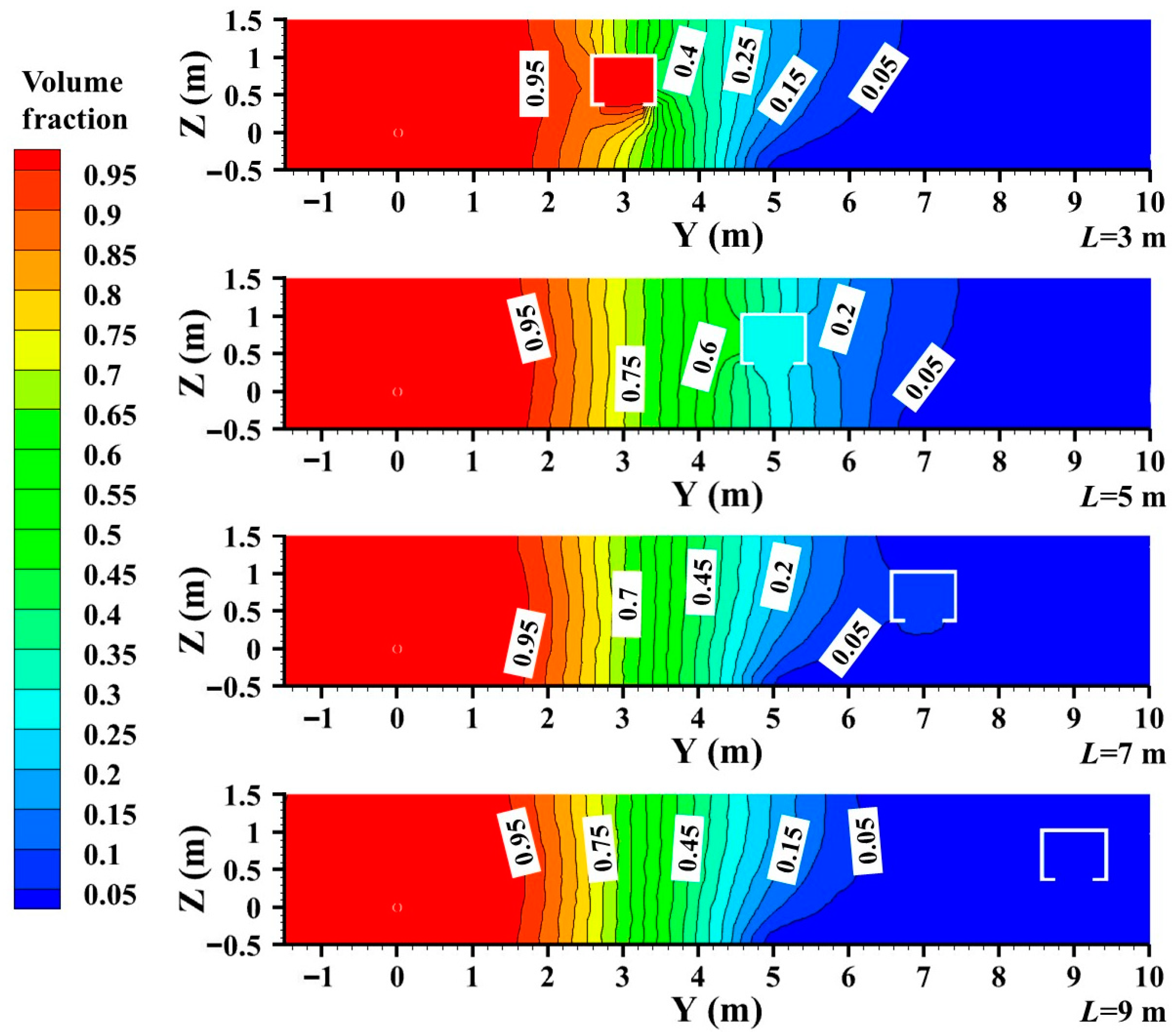
Increasing the pipeline pressure and leakage size enhanced the gas concentration distribution in the confined space. When the pipeline pressure increased from 0.2 MPa to 0.4 MPa, the gas concentration distribution in the confined space enhanced from 15.51% to 29.98%. When the leak diameter enhanced from 20 mm to 60 mm, the gas concentration expanded from 16.05% to 40.02%. Increasing the minimum construction distance between the buried gas pipeline and the confined space reduced the gas concentration distribution in the confined space. When the minimum construction distance increased from 3 m to 9 m, the gas concentration distribution in the confined space decreased from 90.21% to 0.88%.
(3)
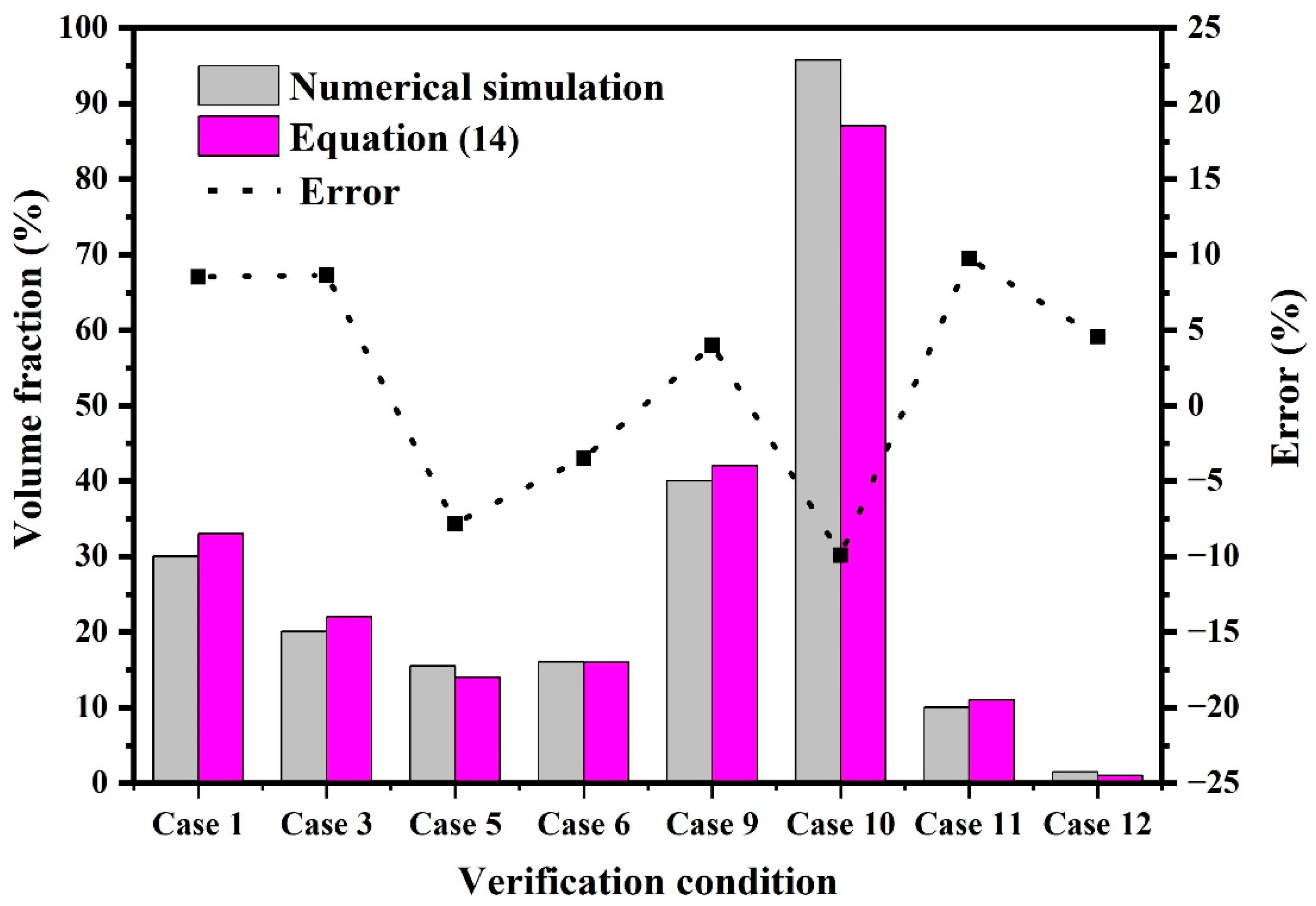
The prediction model for gas concentration in the underground adjacent closed space of the buried gas pipeline leakage was established, and the average error was 4.97%, which can realize the calculation of gas concentration distribution in the closed space under different leakage conditions.
(4)
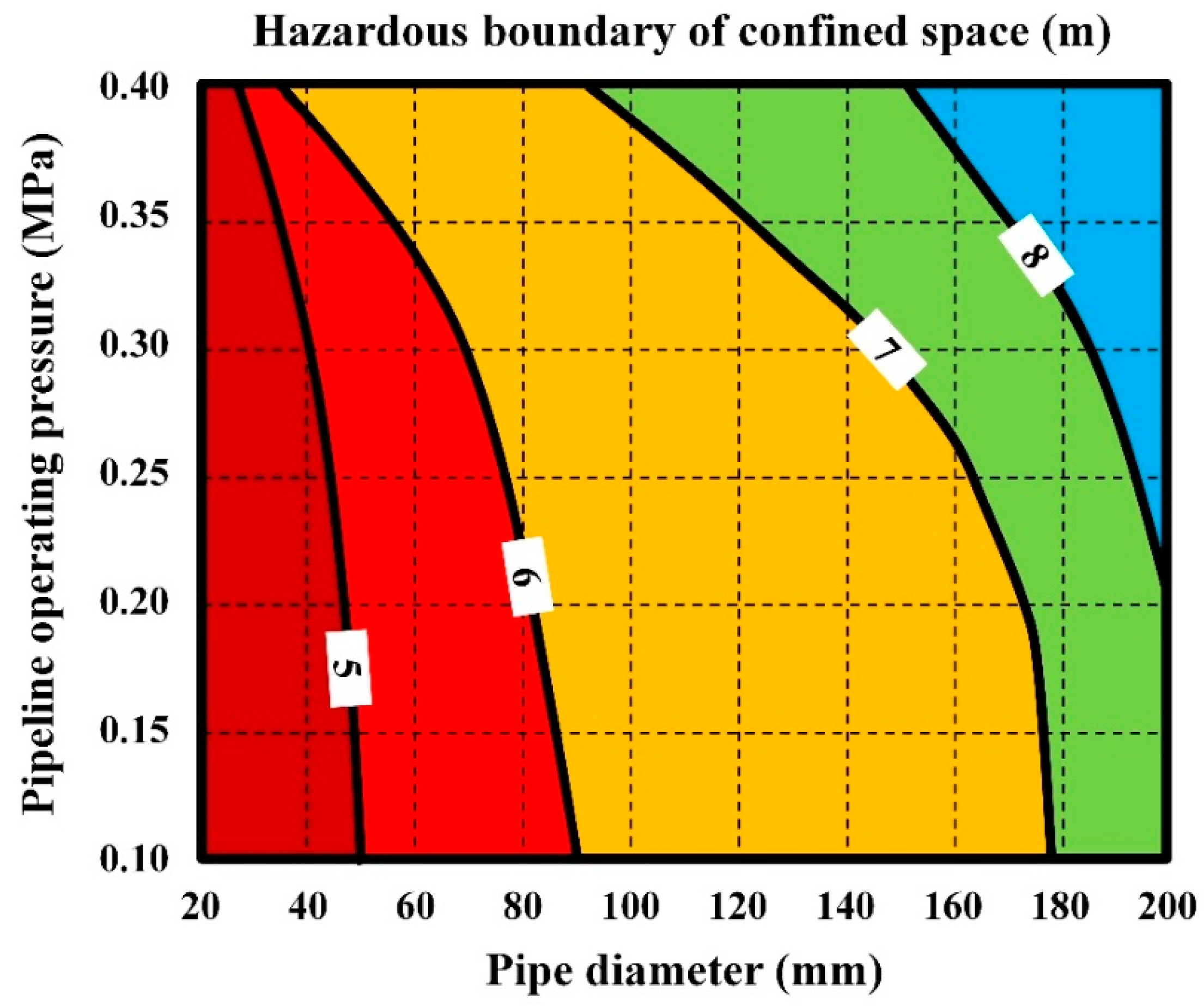
Based on the principle of heavy risk, the calculation model of the hazardous boundary in a confined space was deduced and established by using the gas concentration prediction model, and the hazardous boundary drawing board was further drawn, which realized the rapid determination of the safety distance between the design and construction of a buried gas pipeline, and provided a more scientific basis for the design of the safety distance between a gas pipeline and a confined space in underground engineering construction.
(5)
This paper studied the continuous leakage and diffusion process of gas after the leakage of buried pipelines, and analyzed the distribution and danger of gas entering the confined space. However, the gas diffusion process after closing the valve in case of a leakage accident has not been paid attention to yet. The next step is to analyze the free dissipation process of gas after cutting off the valve at the upstream gas supply end, and effectively defining the hazard duration and range.

Author Contributions

Conceptualization, S.C.; Data curation, Y.L.; Formal analysis, F.B.; Methodology, F.B.; Project administration, Z.W. and S.C.; Resources, Z.W. and H.D.; Software, J.Z.; Supervision, H.L.; Visualization, Z.X. and Y.W.; Writing—original draft, F.B.; Writing—review & editing, F.B. All authors have read and agreed to the published version of the manuscript.

Funding

This research was supported by Research on integrity management technology of urban gas distribution pipeline (2021DJ2806).

Conflicts of Interest

The authors declared that they do not have any commercial or associative interest that represents a conflict of interest in connection with the work submitted.

References

  1. Boswell, R.; Collett, T.S. Current perspectives on gas hydrate resources. Energy Environ. Sci. 2011, 4, 1206–1215. [Google Scholar] [CrossRef]
  2. You, K.; Flemings, P.B.; Malinverno, A.; Collett, T.S.; Darnell, K. Mechanisms of methane hydrate formation in geological systems. Rev. Geophys. 2019, 57, 1146–1196. [Google Scholar] [CrossRef]
  3. Aguilera, R.F. The role of natural gas in a low carbon Asia Pacific. Appl. Energy 2014, 113, 1795–1800. [Google Scholar] [CrossRef]
  4. Biezma, M.V.; Agudo, D.; Barron, G. A fuzzy logic method: Predicting pipeline external corrosion rate. Int. J. Press. Vessel. Pip. 2018, 163, 55–62. [Google Scholar] [CrossRef]
  5. Parvini, M.; Gharagouzlou, E. Gas leakage consequence modeling for buried gas pipelines. J. Loss Prev. Process Ind. 2015, 37, 110–118. [Google Scholar] [CrossRef]
  6. Bu, F.X.; Liu, Y.; Chen, S.Q.; Wu, J.; Guan, B.; Zhang, N.; Lin, X.Q.; Liu, L.; Cheng, T.C.; Shi, Z.C. Real scenario analysis of buried natural gas pipeline leakage based on soil-atmosphere coupling. Int. J. Press. Vessel. Pip. 2022, 199, 104713. [Google Scholar] [CrossRef]
  7. Fan, Y.; van Perry, S.; Klemes, J.J.; Lee, C.T. A review on air emissions assessment: Transportation. J. Clean. Prod. 2018, 194, 673–684. [Google Scholar] [CrossRef]
  8. Badida, P.; Balasubramaniam, Y.; Jayaprakash, J. Risk evaluation of oil and natural gas pipelines due to natural hazards using fuzzy fault tree analysis. J. Nat. Gas Sci. Eng. 2019, 66, 284–292. [Google Scholar] [CrossRef]
  9. Hoeks, J. Effect of leaking natural gas on soil and vegetation in urban areas. Soil Sci. 1975, 120, 317–318. [Google Scholar] [CrossRef]
  10. Lovreglio, R.; Ronchi, E.; Maragkos, G.; Beji, T.; Merci, B. A dynamic approach for the impact of a toxic gas dispersion hazard considering human behaviour and dispersion modelling. J. Hazard. Mater. 2016, 318, 758–771. [Google Scholar] [CrossRef]
  11. Wakoh, H.; Hirano, T. Diffusion of leaked flammable-gas in soil. J. Loss Prev. Process Ind. 2011, 4, 260–264. [Google Scholar] [CrossRef]
  12. Houssin-Agbomson, D.; Blanchetiere, G.; McCollum, D. Consequences of a 12-mm diameter high pressure gas release on a buried pipeline. Experimental setup and results. J. Loss Prev. Process Ind. 2018, 54, 183–189. [Google Scholar] [CrossRef]
  13. Pokhrel, D.; Hettiaratchi, P.; Kumar, S. Methane diffusion coefficient in compost and soil-compost mixtures in gas phase biofilter. Chem. Eng. J. 2011, 169, 200–206. [Google Scholar] [CrossRef]
  14. Wilkening, H.; Baraldi, D. CFD modelling of accidental hydrogen release from pipelines. Int. J. Hydrogen Energy 2007, 32, 2206–2215. [Google Scholar] [CrossRef]
  15. Bezaatpour, J.; Fatehifar, E.; Rasoulzadeh, A. CFD investigation of natural gas leakage and propagation from buried pipeline for anisotropic and partially saturated multilayer soil. J. Clean. Prod. 2020, 277, 123940. [Google Scholar] [CrossRef]
  16. Bu, F.X.; Chen, S.Q.; Liu, Y.; Guan, B.; Wang, X.W.; Shi, Z.C.; Hao, G.W. CFD analysis and calculation models establishment of leakage of natural gas pipeline considering real buried environment. Energy Rep. 2022, 8, 3789–3808. [Google Scholar] [CrossRef]
  17. Bu, F.X.; Liu, Y.; Chen, S.Q.; Xu, Z.; Liu, Y.B.; Jiang, M.H.; Guan, B. Analysis and prediction of methane invasion distance considering real ground boundary. ACS Omega 2021, 6, 29111–29125. [Google Scholar] [CrossRef]
  18. Pontiggia, M.; Derudi, M.; Alba, M.; Scaioni, M.; Rota, R. Hazardous gas releases in urban areas: Assessment of consequences through CFD modelling. J. Hazard. Mater. 2010, 176, 589–596. [Google Scholar] [CrossRef]
  19. Sklavounos, S.; Rigas, F. Estimation of safety distances in the vicinity of fuel gas pipelines. J. Loss Prev. Process Ind. 2006, 19, 24–31. [Google Scholar] [CrossRef]
  20. Tan, Q.; Feng, G.L.; Yuan, H.Y.; Su, G.F.; Fu, M.; Zhu, Y.P. Applied research for the gas pipeline installation and the monitoring method for the safety of the adjacent under-ground spaces. J. Saf. Environ. 2019, 19, 902–908. [Google Scholar]
  21. Ebrahimi-Moghadam, A.; Farzaneh-Gord, M.; Deymi-Dashtebayaz, M. Correlations for estimating natural gas leakage from above-ground and buried urban distribution pipelines. J. Nat. Gas Sci. Eng. 2016, 34, 185–196. [Google Scholar] [CrossRef]
  22. Ebrahimi-Moghadam, A.; Farzaneh-Gord, M.; Arabkoohsar, A.; Moghadam, A.J. CFD analysis of natural gas emission from damaged pipelines: Correlation development for leakage estimation. J. Clean. Prod. 2018, 199, 257–271. [Google Scholar] [CrossRef]
  23. Water Supply and Drainage Design Manual Volume 5, Urban Drainage; China Construction Industry Press: Beijing, China, 1986.
  24. Montiel, H.; Vílchez, J.A.; Casal, J.; Arnaldos, J. Mathematical modelling of accidental gas releases. J. Hazard. Mater. 1998, 59, 211–233. [Google Scholar] [CrossRef]
  25. Luo, J.H.; Zheng, M.; Zhao, X.W.; Huo, C.Y.; Yang, L. Simplified expression for estimating release rate of hazardous gas from a hole on high-pressure pipelines. J. Loss Prev. Process Ind. 2006, 19, 362–366. [Google Scholar] [CrossRef]
  26. Deng, Y.J.; Hu, H.B.; Yu, B.; Sun, D.L.; Hou, L.; Liang, Y.T. A method for simulating the release of natural gas from the rupture of high-pressure pipelines in any terrain. J. Hazard. Mater. 2018, 342, 418–428. [Google Scholar] [CrossRef]
  27. Liu, A.H.; Huang, J.; Li, Z.W.; Chen, J.Y.; Huang, X.F.; Chen, K.; Xu, W.B. Numerical simulation and experiment on the law of urban natural gas leakage and diffusion for different building layouts. J. Nat. Gas Sci. Eng. 2018, 54, 1–10. [Google Scholar] [CrossRef]
  28. Pereira, T.W.C.; Marques, F.B.; Pereira, F.D.R.; Ribeiro, D.D.; Rocha, S.M.S. The influence of the fabric filter layout of in a flow mass filtrate. J. Clean. Prod. 2016, 111, 117–124. [Google Scholar] [CrossRef]
  29. Bu, F.X.; Liu, Y.; Liu, Y.B.; Xu, Z.; Chen, S.Q.; Jiang, M.H.; Guan, B. Leakage diffusion characteristics and harmful boundary analysis of buried natural gas pipeline under multiple working conditions. J. Nat. Gas Sci. Eng. 2021, 94, 104047. [Google Scholar] [CrossRef]
  30. Wang, X.M.; Tan, Y.F.; Zhang, T.T.; Xiao, R.; Yu, K.C.; Zhang, J.D. Numerical study on the diffusion process of pinhole leakage of natural gas from underground pipelines to the soil. J. Nat. Gas Sci. Eng. 2021, 87, 1–14. [Google Scholar] [CrossRef]
  31. GB 50028-2006; Code for Design of City Gas Engineering. Codeofchina Inc.: Beijing, China, 2022.
  32. Okamoto, H.; Gomi, Y. Empirical research on diffusion behavior of leaked gas in the ground. J. Loss Prev. Process Ind. 2011, 24, 531–540. [Google Scholar] [CrossRef]
  33. Torii, S. Numerical simulation of turbulent jet diffusion flames by means of two-equation heat transfer model. Energy Convers. Manag. 2001, 42, 1953–1962. [Google Scholar] [CrossRef]
  34. Jacobsen, Ø.; Magnussen, B.F. 3-D numerical simulation of heavy gas dispersion. J. Hazard. Mater. 1987, 16, 215–230. [Google Scholar] [CrossRef]
  35. Rieger, J.; Weiss, C.; Rummer, B. Modelling and control of pollutant formation in blast stoves. J. Clean. Prod. 2015, 88, 254–261. [Google Scholar] [CrossRef]
  36. Zhang, J.W.; Yin, X.X.; Xin, Y.A.; Zhang, J.; Zheng, X.P.; Jiang, C.M. Numerical Investigation on Three-dimensional Dispersion and Conversion Behaviors of Silicon Tetrachloride Release in the Atmosphere. J. Hazard. Mater. 2015, 288, 1–16. [Google Scholar] [CrossRef]
  37. Nahavandi, N.N.; Farzaneh-Gord, M. Numerical simulation of filling process of natural gas onboard vehicle cylinder. J. Braz. Soc. Mech. Sci. Eng. 2014, 36, 837–846. [Google Scholar] [CrossRef]
  38. Lu, J.S.; Xu, S.; Deng, J.J.; Wu, W.F.; Wu, H.X.; Yang, Z.B. Numerical prediction of temperature field for cargo containment system (CCS) of LNG carriers during pre-cooling operations. J. Nat. Gas Sci. Eng. 2016, 29, 382–391. [Google Scholar] [CrossRef]
  39. Liu, Y.; Bu, F.X.; Chen, S.Q.; Jiang, M.H. Investigating effect of polymer concentrations on separation performance of hydrocyclone by sensitivity analysis. Energy Sci. Eng. 2021, 9, 1202–1215. [Google Scholar] [CrossRef]
  40. Liu, L.; Zhao, L.X.; Reifsnyder, S.; Gao, S.; Jiang, M.Z.; Huang, X.Q.; Jiang, M.H.; Liu, Y.; Rosso, D. Analysis of Hydrocyclone Geometry via Rapid Optimization based on Computational Fluid Dynamics. Chem. Eng. Technol. 2021, 44, 1693–1707. [Google Scholar] [CrossRef]
  41. Nordlund, M.; Stanic, M.; Kuczaj, A.K.; Frederix, E.M.A.; Geurts, B.J. Improved PISO algorithms for modeling density varying flow in conjugate fluid-porous domains. J. Comput. Phys. 2016, 306, 199–215. [Google Scholar] [CrossRef]
  42. Jarrahian, A.; Heidaryan, E. A new cubic equation of state for sweet and sour natural gases even when composition is unknown. Fuel 2014, 134, 333–342. [Google Scholar] [CrossRef]
  43. Sarkar, A.; Dey, P.; Rai, R.N.; Saha, S.C. A comparative study of multiple regression analysis and back propagation neural network approaches on plain carbon steel in submerged-arc welding. Sadhana 2016, 27, 82–89. [Google Scholar] [CrossRef] [Green Version]
Figure 1. Schematic diagram of the physical model.
Energies 15 06859 g001
Figure 2. Schematic diagram of spatial location of monitoring points.
Energies 15 06859 g002
Figure 3. (a) CH4 concentration comparison at Coordinate A. (b) CH4 concentration comparison at Coordinate B.
Energies 15 06859 g003
Figure 4. (a) Pressure distribution curves of monitoring points inside the pipeline. (b) Pressure distribution curves of monitoring points outside the pipeline.
Energies 15 06859 g004
Figure 5. Cloud diagram of pressure distribution at different leakage times.
Energies 15 06859 g005
Figure 6. (a) Velocity distribution curves of monitoring points inside the pipeline. (b) Velocity distribution curves of monitoring points outside the pipeline.
Energies 15 06859 g006
Figure 7. Cloud diagram of velocity distribution at different leakage times.
Energies 15 06859 g007
Figure 8. Cloud diagram of streamline distribution with different leakage time on plane Y = 0.
Energies 15 06859 g008
Figure 9. Cloud diagram of streamline distribution with different leakage time on plane X = 0.
Energies 15 06859 g009
Figure 10. Cloud diagram of gas concentration distribution in confined space at different leakage times.
Energies 15 06859 g010
Figure 11. Gas concentration change curve at monitoring point 5.
Energies 15 06859 g011
Figure 12. Schematic diagram of hazardous boundary of buried gas pipeline and underground confined space.
Energies 15 06859 g012
Figure 13. Influence of minimum construction distance L on gas concentration distribution in confined space.
Energies 15 06859 g013
Figure 14. The influence of pipeline operating pressure and leakage diameter on gas concentration distribution in confined space.
Energies 15 06859 g014
Figure 15. Validation of gas concentration prediction model in confined space.
Energies 15 06859 g015
Figure 16. Hazardous boundary drawing board.
Energies 15 06859 g016
Table 1. Working conditions.
Casep (MPa)d (mm)L (m)
10.4405
20.35405
30.3405
40.25405
50.2405
60.4205
70.4305
80.4505
90.4605
100.4403
110.4407
120.4409
Table 2. Boundary condition definition.
Boundary LocationBoundary Type
Pipe inletPressure inlet
Pipe outletPressure outlet
Soil boundaryPressure outlet
Local encryption boundaryInterface
Leakage hole of buried pipeline and confined spaceInterior
Confined space sidewallWall
Table 3. Grid independence verification.
Grid LevelGrid NumberLeakage RateError
1514,7840.004738 kg/s/
21,133,6620.004456 kg/s7.66%
31,502,3390.004352 kg/s2.39%
41,887,4510.004319 kg/s0.76%
Table 4. Characteristic parameters of different buried media.
Buried MediumPorosity (%)Permeability (m2)Diffusion Coefficient (m2/s)
Asphalt5.00.40.21
Crushed stone23.54.12.23
Pit sand17.02.00.66
Table 5. Correlation analysis.
CoefficientEstimated ValueConfidence Interval
β 0 −247.4878[−367.6461, −127.3294]
β 1 −9.3133[−15.0174, −3.6092]
β 2 3832.7156[1581, 6085]
β 3 80.0360[43.3944, 116.6775]
R2 = 0.9109   F = 1.4350 × 10³P = 0
Publisher’s Note: MDPI stays neutral with regard to jurisdictional claims in published maps and institutional affiliations.

