Heat Transfer Characteristics of an Aeroengine Turbine Casing Based on CFD and the Surrogate Model

Abstract

A good turbine casing cooling design should control the thermal stress and maintain a reasonable tip clearance between the turbine blade and the casing. Since the turbine inlet temperature has been increased yearly, the influence of thermal radiation on the temperature of a turbine casing has become more significant. Therefore, the heat transfer characteristics of a turbine casing considering the radiation effect need to be precisely predicted. In this study, a theoretical model is established for describing the heat transfer characteristics of a turbofan casing, and the model’s effectiveness is verified by comparing the numerical and experimental results. Based on the validated model, the effects of single changes of the wall temperature, cooling air temperature, Reynolds number, and surface emissivity on the heat transfer of the casing are discussed. The results show that the increment of cooling air temperature and surface emissivity leads to the enhancement of the average radiative Nusselt number, and the average convective Nusselt number increases as the Reynolds number increases. The emissivity can improve the temperature distribution uniformity of the turbine casing. Finally, a Kriging surrogate model is fitted with 20 sample points to predict the joint effect of multiple parameters on the casing surface Nusselt number. It is found that the Reynolds number has a more significant influence on the average Nusselt number compared with the emissivity and the temperature ratio.

1. Introduction

To improve the performance of the aeroengine, the gas turbine inlet temperature continues to increase, which leads to a more severe thermal environment for the turbine components. As an integral part of the turbine components, the turbine casing experiences mechanical and thermal loads. Some parts are in direct contact with gas and can be affected by the aerodynamic heat, resulting in radial deformation, which can lead to the change in the tip clearance. The tip clearance is the gap between the turbine blade and the casing. An unreasonable tip clearance will reduce the engine efficiency and increase the cost of fuel [1,2]. A good casing cooling design should control the thermal stress and maintain a reasonable tip clearance between the turbine blade and the casing. The cooling air is drawn from the compressor and divided into two streams [3]: the external cooling flow and the internal cooling flow. The former cools the external casing, and the latter flows into the cavity surrounded by a multi-layer casing to cool the casing. For the external impinge cooling issues, considerable research has been conducted. For example, Da Soghe and Andreini [4] explored the aerodynamic losses of jet array holes with a simulation and developed an empirical correlation for the discharge coefficient with several feeding pipe geometry parameters. Finally, they verified the availability of this expression by comparison between the experiment and CFD. Tapanlis et al. [5] numerically studied the condition of the casing deformations with different jet cooling mass flow rates and obtained the correlation relationship for the area averaged Nusselt numbers with various flow rates and geometry parameters. Choi et al. [6,7] systematically studied the influence of a range of impingement cooling arrangements on a casing closure and obtained the heat transfer coefficient of the external casing surface, and they studied the heat transfer with the distance variation of the external casing and the manifold.

In addition, numerous experimental and numerical studies on the internal cooling flow in casing cavities and the heat transfer between the casing and the fluid have been conducted. Pilkington et al. [8,9] studied the thermal protection method for a casing with the leading effect of natural convection during the shutdown of industrial gas turbines with numerical calculation. They also proposed a method for extracting the fluid from the upper hole of the casing. This method could reduce the disadvantage of small heat flux at the top of the casing caused by natural convection, enhance the heat transfer flow at the top of the casing, and reduce the deformation of the casing caused by thermal stress. In addition, they designed a simplified casing model that could simulate the natural convection phenomenon in the casing for the actual Rayleigh number conditions. They developed a modified gradient diffusion hypothesis model, GGDH+, which can be used to explain the effects of buoyancy on turbulent heat flow. Murat et al. [10] designed a novel piece of experimental equipment for testing the mixed flow field of a turbine casing and found that laminar flow to the turbulence transition caused by buoyancy occurred from the lower part of the casing to the upper part of the casing.

Turbine casings are usually multi-annulus structures that often contain closed ring structures. Given the heat transfer situation of closed annulus structures, some scholars have conducted the following studies. Shaija and Narasimham [11] studied the influence of considering whether the surface was radioactive or not on the natural convection heat transfer in a horizontal cylindrical annulus through numerical calculation. The results showed that the natural convective heat transfer performance in the annulus decreased with the surface radiation. However, the overall Nusselt number on the inner wall surface increased significantly compared with that without consideration of the surface radiation effect. The Rayleigh number of the fluid in a horizontal concentric annulus is the most important dimensionless parameter and is mainly affected by the physical properties of the fluid and the temperature difference. When the critical Reynolds number is exceeded, the dual steady-state solution is generated [12]. Owen [13] studied the flow field driven by buoyancy in the closed cavity between the adjacent disks of a compressor rotor through numerical calculation and derived the equation of the entropy production rate.

The parameters that affect the heat transfer characteristics of a turbine casing include the Reynolds number, cooling air temperature, wall rib structures, and other parameters. Some scholars have explored the influence of the Reynolds number [14], embedded bolts [15], surface rib structure [16], and other parameters on the convection heat transfer inside the casing. For example, Tong et al. [16] studied the heat transfer effects of four surface roughness structures of impingement target plates in the periodic structure of a turbine casing using numerical methods. The results showed that the cooling effect of the surface roughness structure was better than that of a smooth surface in the range of multiple impingement cooling systems. The heat transfer effect of the cambered rib configuration was the best. Its average Nusselt number was up to 62.6% higher than that of a smooth wall. With the continuous rise of the turbine front temperature, the influence of the casing surface emissivity cannot be ignored [17].

Given the above, there have been numerous studies on the heat transfer of external cooling flow on the external casing of an aeroengine. However, there are few studies on flow in a casing annulus cavity and the heat transfer characteristics of a casing for the aeroengine. Existing studies are primarily limited to the industrial gas turbine and steam turbine fields. Unlike the latter two categories, an aeroengine turbine casing includes closed annulus structures; furthermore, it works at a higher turbine inlet temperature, where the radiation heat transfer between the casing surfaces cannot be ignored [18]. Thus, the coupling mechanism of the casing surface radiation, convective heat transfer, and heat conduction at high temperatures is still unclear. Therefore, it is important to study the heat transfer characteristics of an aeroengine casing by employing experiments and simulations for a good inner cooling design.

This study establishes a numerical model for describing the heat transfer characteristics of a turbofan casing, and the model’s effectiveness is verified by comparing the numerical and experimental results. Based on this model, we study the heat transfer characteristics of this turbine casing with the single variation, including the wall temperature, cooling air temperature, Reynolds number, and surface emissivity. Finally, the Kriging surrogate model is adopted to study the joint effect of multiple parameters on the heat transfer characteristics of the casing. Based on the research above, the casing’s temperature and Nusselt number distribution can be precisely predicted, which can help design a good turbine casing cooling system.

2. Physical and Math Models

2.1. Physical Model

The simplified turbine casing model without hooks is shown in Figure 1. The casing is divided into two parts, the open annulus and the closing annulus, because these parts have different heat transfer characteristics, which are studied in this work.

The size parameters of the holes in Figure 1 are shown in

Table 1. Geometrical parameters of the holes in the casing.

Geometry	Parameter
Hole 1	Φ34 (mm) × 10
Hole 2	Φ4 (mm) × 20
Hole 3	Φ2 (mm) × 20
Hole 4	Φ6 (mm) × 40
Hole 5	Φ3 (mm) × 40
Square hole	7 (mm) × 1 (mm) × 42

.

2.2. Governing Equations and Boundary Conditions

The air is simplified as an ideal gas, and this model has been applied to previous heat transfer problems of high-pressure turbine components [19]. The kinematic viscosity of the air obeys the Sutherland formula [20]. In this study, the change in other physical properties of the air is not significant, and the physical properties of the air and casing are fixed. Their values are shown in

Table 2. The physical properties of the casing and the air.

Material	Physical Quantity	Value
Turbine casing	$\rho$ (kg/m3)	8240
	Cp (J/(kg K)	550
	$\lambda$ (W/(m K))	22
Air	Cp (J/(kg K)	1110
	$\lambda$ (W/(m K))	0.06

.

As the average flow velocity exceeds 0.3 Ma at the casing outlet, the influence of the air compressibility is considered in this study. Additionally, the flow is turbulent, so the governing equations are as follows.

$$\frac{\partial \left(\rho u_i\right)}{\partial x_i}=0,$$

(1)

$$\frac{\partial }{\partial x_j}\left(\rho u_i{u}_j\right)=-\frac{\partial P}{\partial x_i}+\frac{\partial }{\partial x_j}\left(t_{ij}+\rho {\tau }_{ij}\right)+\rho g_i,$$

(2)

$$\frac{\partial \rho u_j{c}_{P}T}{\partial x_j}=\frac{\partial }{\partial x_j}\left(\left(\lambda +\frac{c_P{\mu }_T}{P{r}_T}\right)\frac{\partial T}{\partial x_j}\right)+\frac{\partial }{\partial x_j}\left(\left(t_{ij}+\rho {\tau }_{ij}\right)u_i\right)+\rho g_i{u}_i,$$

(3)

where $t_{ij}=2\mu \left(S_{ij}-\frac{1}{3}{S}_{kk}{\delta }_{ij}\right),\rho {\tau }_{ij}=2{\mu }_T\left(S_{ij}-\frac{1}{3}{S}_{kk}{\delta }_{ij}\right)-\frac{2}{3}\rho k{\delta }_{ij}$.

The computational domains include both the solid and fluid domains. For the solid casing, the governing equation only contains the energy equation, and only the heat conduction term exists in the energy equation. In addition, the casing surface is opaque and has a gray surface in this study.

At the solid–liquid interface, the boundary conditions for which the heat flux is continuous and the temperature does not step are:

$$-\lambda \frac{\partial T_s}{\partial x_j}=S_r+S_c,$$

(4)

where

$$S_r={\epsilon }_w\sigma T_w^4+\frac{\left(1-{\epsilon }_w\right)}{\pi }{{\displaystyle \int }}_{s_i\cdot n_w<0}\sigma T_i^4\left|s_i\cdot n_w\right| d{\mathsf{\Omega }}_i.$$

(5)

In this study, the surface temperature of the inner annulus of the casing is set to be constant, and the remaining surfaces are set to be fixed with a heat transfer coefficient of 320 W/m² K and an environment temperature of 600 K. The effects of the wall temperature, cooling air temperature, Reynolds number, and wall emissivity on the heat transfer characteristics of the casing are studied. The values of these parameters are shown in

Table 3. Values of parameters.

Parameter	Value
Wall temperature/K	900, 1100, 1300
Cooling air temperature/K	700, 800, 900
Reynolds number	39,800, 59,700, 79,600
Surface emissivity	0, 0.4, 0.6, 0.8
Outlet average static pressure/Pa	1,041,325

.

2.3. Numerical Solution and Validations

The turbulence model needs to be selected to close the Navier–Stokes equations. Since the flow in the casing cavity is a mostly impinging jet, considering the high accuracy of the shear stress transport (SST) model in predicting the jet problem, this model is selected as the turbulence model in this study. Given that the physical domain is very complex, the Discrete Ordinate Method (DO) [21] is adopted as the radiation model. However, its accuracy is subject to the number of discretized angles and pixels. This study selects the combination of 4 × 4 controlled angles and 3 × 3 pixels, which is a trade-off between computational resources and accuracy. The commercial computational fluid dynamics software, Fluent, is used as the solver to solve the discrete Navier–Stokes equations. The gradients are computed with the Green–Gauss cell-based method, and the pressure interpolation scheme is the pressure staggering option. Additionally, other spatial discretization schemes are set for the second-order upwind. After that, the solution scheme for the pressure–velocity coupling is the Couple scheme, which can improve the convergence.

A comparison of the CFD and the experiments is conducted to verify the precision of the numerical models. The experimental devices are shown in Figure 2:

As shown in the figure, the experimental system mainly includes an experiment rig, a data acquisition device, a temperature controlling device, and devices for measuring flow and pressure. The experiment rig consists of a simplified casing and a heater, which, compared to the numerical geometry model, the simplified casing adds an inlet air collection cavity and an outer air collection cavity. Moreover, the experimental material used in this paper is austenitic 304 stainless steel. The heater consists of a ring of heated magnetic beads, which can provide uniform heat flux. The data acquisition device is an Agilent 34,970 A, which records the inlet air temperature, wall surface temperature, and cavity temperature. Meanwhile, a bypass line control valve controls the mass flow rate displayed on the flowmeter. The primary working process is as follows.

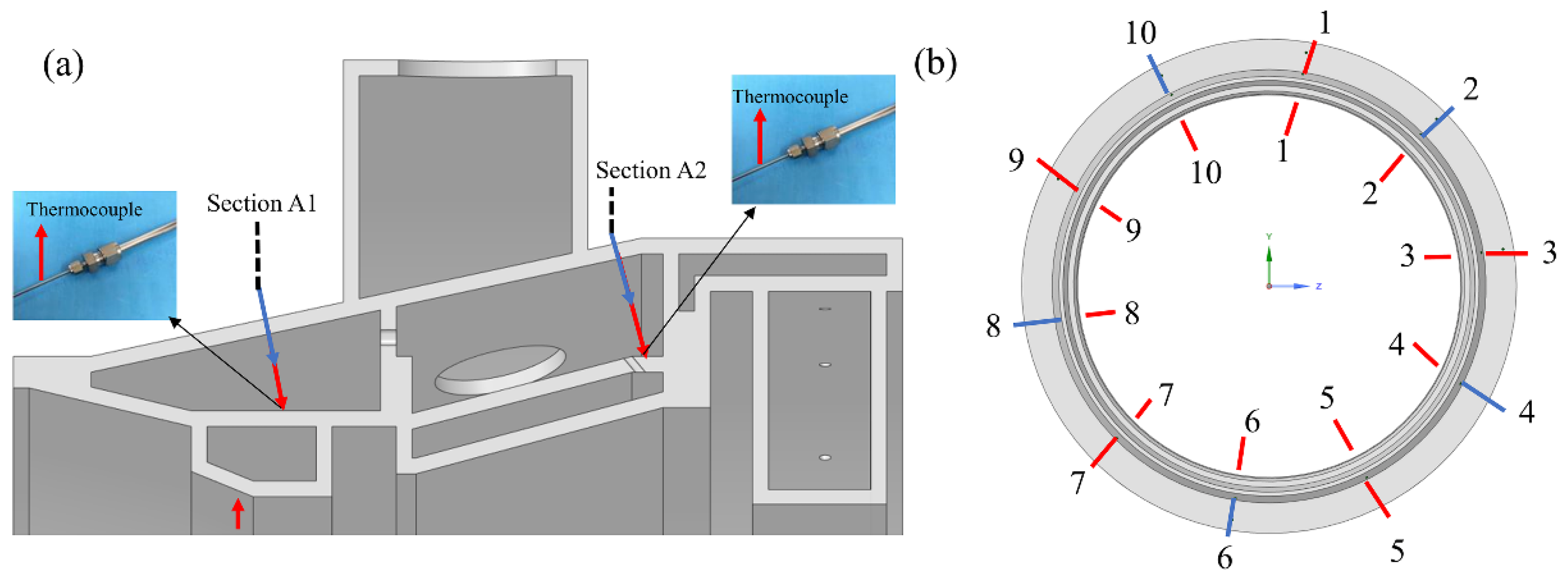
An axial flow compressor firstly compresses the air, and it flows to the air heater, where it is heated. Then, the heated air delivered by pipes enters the air collection cavity through five inlets, cooling the casing wall heated by the heater. Finally, it is discharged through the tail gas treating unit. K-type armored thermocouples are used to measure the temperature of the inlet air, casing surface, and cavity. Their distribution positions on the casing are shown in Figure 3.

The blue arrows represent the thermocouples for measuring the cavity temperatures, and the red arrows represent the thermocouples for measuring the wall surface temperatures. There are ten thermocouples evenly distributed in the closed cavity formed by the heater and the inner annulus of the casing. When the wall process reaches a steady state, it can be considered that the average temperature of the thermocouples is the same as the average temperature of the inner annulus surface of the casing. The thermocouple at position one directly connects with the temperature controlling device to measure the heating temperature, and the other nine thermocouples connect with the data collector. Due to the natural convection effect, the thermocouple temperatures in the upper part of the cavity are higher than those in the lower part. The thermocouple temperatures are set as the temperature boundary condition of the inner annulus surface of the casing for the numerical simulation.

Additionally, there are ten thermocouples evenly distributed in the circumferential direction of Section A1 and Section A2, of which five thermocouples are used to measure the cavity temperatures and five thermocouples are used to measure the wall temperatures. The thermocouples, which measure the temperature of the wall surface, are fixed to the wall surface by the structure shown in the upper left and upper right corners of Figure 3. The number of grids used for validation is 17.2 million. The boundary layer has ten layers of grids, which can capture sharp changes in temperature in the boundary layer region. The average y+ of the first layer is less than 1, and the turbulence model can well capture the flow near the wall.

The mass flow rate and thermocouple temperatures are directly measured data. A high-precision flowmeter with an uncertainty of ±1% is used to measure the mass flow rate. The temperature uncertainty consists of K-type armored thermocouples and the data acquisition system, wherein the former has an accuracy of ±2.5 K and the latter has an accuracy of ±1.0 K. As a result, the estimated temperature uncertainty varies from ±0.5% to ±0.7% for the measuring temperature ranging from 499.1 K to 682.8 K.

The geometry model used as the numerical validation is shown in Figure 3a, which has the same size as the experiment model. Two schemes of results are compared for the experiment and the simulation. Scheme 1 corresponds to the heating temperature of 850 K, the inlet temperature of 495 K, and the mass flow rate of 0.1 kg/s; Scheme 2 corresponds to the heating temperature of 935 K, the inlet temperature of 500 K, and the mass flow rate of 0.4 kg/s. The two schemes have the same outlet pressure of 101,325 Pa, and the outer annulus surfaces of the casing are set at a fixed heat transfer coefficient of 10 W/m² K and an environment temperature of 300 K. The emissivity of the casing wall is referenced in [22], which is 0.4. The heating temperature is read from the temperature controlling device.

For the two working conditions, at the positions of Section A1 and Section A2, the comparison between the experimentally-measured thermocouple temperatures and the simulated temperatures is shown in Figure 4 and Figure 5.

It can be seen from Figure 4 and Figure 5 that the temperature differences between the experiment and the simulation calculation is within 5.5%. The difference is partly because of the radiation effect between the thermocouple and the casing. Additionally, it should not be ignored that the thermocouple dissipates part of the heat into the environment through heat conduction. To summarize, it can be considered that the numerical results have good agreement with the experiment. It is reliable to use the numerical model to calculate the comprehensive heat transfer problem of the turbine casing.

2.4. Grid Independence Check

Figure 6 shows the average temperature and Nusselt number with different grid numbers corresponding to 8,988,841, 11,310,415, 15,598,636, and 17,425,511 cells for Case 5. Finally, grid_3 with 15,598,636 cells is adopted as the computational mesh, which has enough accuracy and a lower computational cost.

2.5. Definition of Dimensionless Numbers

In order to make the conclusion of this study more general, several dimensionless numbers that are closely related to the flow and heat transfer are defined. The Nusselt number is defined as follows:

$$Nu=\frac{\left(h_c+h_r\right)L}{\lambda },$$

(6)

$$h_c=\frac{-\lambda \frac{\partial T}{\partial n}}{\mathsf{\Delta }T},$$

(7)

$$h_r=\frac{{\epsilon }_W\sigma T_W{}^4+{\epsilon }_W{\int }_{2\pi }{I}_{in}n·s_{i}d{\mathsf{\Omega }}_i}{\mathsf{\Delta }T},$$

(8)

where $\mathsf{\Delta }T$ is the expression of temperature difference and L is the characteristic length. For the open annulus, L is the maximum radius $L_1$ of the casing and the temperature difference is defined as follows:

$$\mathsf{\Delta }{T}_1=T_W-T_{in,total},$$

(9)

where $T_W$ is the average temperature of the casing surface and $T_{in,total}$ is the total temperature of the cooling air.

For the closed annulus, L is the maximum radius $L_2$, and the temperature difference is defined as follows:

$$\mathsf{\Delta }{T}_2=T_i-T_o,$$

(10)

where $T_i$ is the average temperature of the inner surface of the inner annulus of the closed annulus and $T_o$ denotes the average temperature of the inner surface of the outer annulus of the closed annulus.

The Reynolds number of the flow is defined as follows:

$$\mathrm{Re}=\frac{U{L}_1}{\nu }=\frac{4\dot{m}}{n\pi L_1\mu }.$$

(11)

The Grashof number that is closely associated with the natural convection of air in the annulus cavity is defined as follows:

$$Gr=\frac{g\beta \left(T_W-T_f\right)L_2{}^3}{{\nu }^2}.$$

(12)

3. Results and Discussion

In order to simplify the calculation, the physical model of this numerical study omits the inlet and outlet air collection cavities, as shown in Figure 1. Numerical calculations will be conducted based on the model from Section 2.1 and Section 2.2. The following ten simulations are conducted with different wall temperatures, cooling air temperatures, emissivity, and Reynolds numbers to obtain the heat transfer characteristics of the casing. The simulation examples discussed in this paper are shown in

Table 4. Simulation examples.

Case	Wall Temperature	Cooling Air Temperature	Emissivity	Re
Case 1	900 K	700 K	0.4	39,800
Case 2	1100 K	700 K	0.4	39,800
Case 3	1300 K	700 K	0.4	39,800
Case 4	1100 K	800 K	0.4	39,800
Case 5	1100 K	900 K	0.4	39,800
Case 6	1100 K	700 K	0	39,800
Case 7	1100 K	700 K	0.6	39,800
Case 8	1100 K	700 K	0.8	39,800
Case 9	1100 K	700 K	0.4	59,700
Case 10	1100 K	700 K	0.4	79,800

.

3.1. Flow and Temperature Field Analysis

Case 5 is used as the baseline case for the flow field and temperature field analysis for convenience. Figure 7 shows the combination of the velocity contour and the temperature contour in the X–Z sections in the fluid domain of the open annulus. As can be seen from the figure, the cooling air vertically impinges on the casing surface. In the stagnation point region of the impingent jet, the casing can be cooled because the thickness of the boundary layer is very thin and the thermal resistance of the boundary layer is small.

With the development of the flow, the cooling air flows into different annular cavities. Its flow is limited by the casing wall, resulting in many vortices and secondary flow structures with different sizes and scales. These vortices and secondary flow structures have different heat transfer effects on the casing.

There are two local high-temperature regions in the left triangular cavity. The main reason is that two fluid streams collided in this region, and the low-velocity fluids with high temperature eject to high-velocity fluids with low temperature. In the cavity above the middle casing, the temperature is mainly affected by the cooling air temperature and the effect of the vortex is little. In the cavity below the middle casing, the temperature of the casing impinged by the cooling air is low. As the boundary layer thickness increases, the convection effect is weakened, and the temperature of the casing increases. Due to the limitation of the casing structure, the flow develops into many secondary flows in this cavity, and their velocities are smaller than that of the main flow. The high temperature cannot be transported promptly, and the local heat exchange effect deteriorates.

Figure 8a shows the temperature distribution of wall_1. It can be seen from the figure that the temperature of the region that is vertically impinged by the cooling air is lower than the temperatures in other areas. As Figure 8b shows, the temperature distribution of wall_1 is periodically presented in the circumferential direction, where P_1 represents the position of the maximum value point along the direction of gravity and P_2 is the maximum value point along the opposite direction of gravity. It can be inferred that the influence of gravity on the temperature distribution of wall_1 is minimal and can be ignored.

Figure 9 shows the velocity contour in the Y–Z section of the fluid domain in the closed annulus. Due to the temperature difference between the inner and outer surfaces of the closed cavity, the fluid in the cavity is subject to the natural convection effect. This presents the following characteristics: the air in the upper part flows upward due to the heating from the inner surface and develops towards the lower part along the outer surface, and the fluid in the lower part is heated by the inner surface and flows along the inner surface to the upper part, driven by buoyancy. The two fluids continuously develop the boundary layer depending on the viscous force. Finally, the two boundary layers interact with each other. The boundary layer velocity along the outer surface is higher than that along the inner surface, and the fluid flows toward the lower part as a whole.

Figure 9 shows the velocity contour in the Y–Z section of the fluid domain in the closed annulus. Due to the temperature differences between the inner and outer surfaces of the closed cavity, the fluid in the cavity is subject to the natural convection effect. This presents the following characteristics: in the upper part, the air flows upward due to the heating from the inner surface and develops towards the lower part along the outer surface; in the lower part, the fluid is heated by the inner surface and flows along the inner surface to the upper part, driven by buoyancy. The two fluids continuously develop the boundary layer depending on the viscous force. Finally, the two boundary layers interact with each other. The boundary layer velocity along the outer surface is higher than along the inner surface, and the fluid flows toward the lower part as a whole.

In the middle of the annular cavity, the flow of two types of boundary layers has the lowest resistance and the fastest velocity. The velocity distribution of AB transversal in Figure 9 is shown in Figure 10. The velocity distribution has two peak values. The velocity peak of the boundary layer that is developing close to the outer surface is greater than that of the boundary layer developing close to the inner surface. This is because, for the former, gravity moves in the same direction as the flow, acting as a driving force, while for the latter, gravity blocks the flow.

Figure 11 shows the temperature distribution of the Y–Z section in the annulus cavity. Due to the low velocity of the natural convection caused by the temperature differences between the inner and outer surfaces of the annulus, the corresponding dimensionless Grashof number, which represents the flow state of natural convection, is small. According to the conclusion obtained in the published literature [23], the natural convection in the closed cavity is in a laminar flow state at this time. The heat transfer process from the inner surface to the outer surface only involves heat conduction and surface radiation. Therefore, the temperature distribution in the cavity is uniform, and the isotherms are approximately concentric circles.

3.2. Effect of Wall Temperature on Heat Transfer Characteristics

Figure 12 shows the variation of the average Nusselt numbers with the wall temperature with a fixed cooling air temperature of 700 K, Reynolds number of 39,700, and surface emissivity of 0.4. Figure 12a shows that the average convective Nusselt number increases with the wall temperature, varying from 900 K to 1100 K. The main reason is that the Nusselt number is a ratio between the heat flux and the temperature difference. In this scenario, the numerator increases by a higher multiple than the denominator. However, when the heat temperature varies from 1100 K to 1300 K, the average Nusselt number decreases. In this scenario, the denominator increases by a higher multiple than the numerator. The proportions of the average radiative Nusselt numbers in the average Nusselt number vary with the wall temperature by 10%, 10.3%, and 13%.

What can be seen from Figure 12b is that with the increment of the wall temperature, the average convective Nusselt number is basically constant. The average Nusselt number at 1300 K is 2.8-times greater than that at 900 K. Furthermore, the contribution of the average convective Nusselt numbers to the average Nusselt numbers is negligible. The variation trend of the average Nusselt number with the wall temperature has a positive correlation.

3.3. Effect of Cooling Air Temperature on Heat Transfer Characteristics

Figure 13 shows the variation of the average Nusselt numbers with the cooling air temperature with a fixed wall temperature of 1100 K, Reynolds number of 39,700, and surface emissivity of 0.4. It can be seen that with the increase in the cooling air temperature, the average radiative Nusselt numbers also increase, while the average convective Nusselt numbers remain unchanged. The ratio between the average radiative Nusselt number and the average Nusselt number increases rapidly with the cooling air temperature increment. When the cooling air temperature is 900 K, the ratio is up to 29.1%. The average Nusselt number distribution on wall_2 is essentially not affected by the cooling air temperature. Compared with the wall temperature, the cooling air temperature has a more pronounced influence on the radiative Nusselt number of wall_1.

3.4. Effect of Reynolds Number on Heat Transfer Characteristics

The Reynolds number is a key factor affecting the heat transfer characteristics of the casing. Figure 14 shows the variation in the average Nusselt number with the Reynolds number for wall_1 with a fixed wall temperature of 1100 K, cooling air of 900 K, and surface emissivity of 0.4. It can be seen that with the increment of the Reynolds number, the average radiative Nusselt number basically remains unchanged. In contrast, the average convective Nusselt number keeps increasing. When the Reynolds number increases from 39,800 to 79,600, the average convective Nusselt number increases by 69.8%, and the maximum convective Nusselt number increases by 9.8%. In addition, the change in the Reynolds number has little effect on the Nusselt numbers on wall_2. Figure 15 shows the change in the average temperature of wall_1 for different Reynolds numbers. It can be seen from the figure that with the increase in the Reynolds number, the average temperature of wall_1 decreases from 995 K to 978 K, a decrease of 17 K, and the maximum temperature of wall_1 changes from 1056 K to 1048 K, a decrease of 8 K.

3.5. Effect of Surface Emissivity on Heat Transfer Characteristics

Figure 16 shows the variation of the average Nusselt number with the change of the surface emissivity with a fixed wall temperature of 1100 K, cooling air of 900 K, and Reynolds number of 39,700. It can be seen that with the emissivity increase, the average radiative Nusselt numbers increase sharply, and the convection Nusselt numbers remain unchanged. When the emissivity is 0.8, the average radiative Nusselt numbers account for nearly 45% of the average Nusselt numbers. As the emissivity increases from 0.4 to 0.8, the average radiative Nusselt numbers increase by 133%. Figure 16b shows that the average radiative Nusselt numbers increase by 151% when the emissivity increases from 0.4 to 0.8.

Figure 17 shows the temperature distributions of the X–Y section of the casing for different surface emissivities. It can be intuitively seen that as the emissivity increases, so does the temperature of the outer annulus of the casing. When the emissivity is 0.8, the average surface temperature of the outer annulus of the casing increases by 40 K compared with that of the outer annulus without radiation. This is because the emissivity increases the heat exchange between the casing surfaces; the heat is distributed from the high-temperature surface to the low-temperature surface by radiation, thereby reducing the temperature difference between the casing surfaces.

As shown in Figure 18, the temperature distributions with different surface emissivities are plotted. Point A on the transversal AB represents the point of the dimensionless distance of 0, and point B represents the point with the dimensionless distance of 1. Similarly, points C and D represent the points with the dimensionless distance of 0 and 1, respectively. The line segment with drastic changes in the figure represents the conversion between the cavity and wall temperatures. It can be seen that with the increase of the emissivity, the temperature in the closed annulus cavity decreases. The effect of the emissivity on the temperature in other cavities is not apparent. Within the range of 0.2–0.5 of the AB transversal, the temperature of the cavity without wall surface radiation is lower than that of the cavity with wall surface radiation. The main reason is that the radiation promotes heat transfer between wall surfaces. Furthermore, with the emissivity increment, the cavity’s temperature near the gas side increases while the temperature near the bypass decreases.

4. Joint Effects of Multiple Parameters on the Casing Surface Nusselt Number

It is necessary to study the joint effects of multiple parameters on the casing surface Nusselt number, however, predicting the surface Nusselt number with traditional methods is usually time-consuming and expensive. Many surrogate model methods, such as the support vector regression [24,25], Artificial neural network [26,27], Response Surface [28,29], and Kriging [30,31,32], can replace the work of simulations and experiments. The precision of surrogate models is similar to CFD, but the calculation resources and the design cycle are saved.

According to the above analysis, it can be found that the distribution of the Nusselt numbers on the target surface is related to the Reynolds number, wall temperature, cooling air temperature, and wall emissivity $\epsilon$, namely:

$$N{u}_{avg}=f(T_W,T_{in},\epsilon ,Re)$$

(13)

Based on the analysis in Section 3.2, the effect of wall temperature on the Nusselt number is small. For convenience, the ratio of the cooling air temperature to the wall temperature is expressed by $\alpha$, representing the joint influence of the cooling air temperature and the wall temperature. Therefore, the above equation is converted to the following form:

$$N{u}_{avg}=f\left(\alpha ,\epsilon ,Re\right).$$

(14)

In order to obtain the relationship shown in Equation (14), the Kriging surrogate model is adopted for prediction. This model can utilize known point data to predict unknown point data. It can be expressed as the following formula [33]:

$$\widehat{y}\left(x\right)=F\left(x\right)+G\left(x\right)$$

(15)

where F(x) is usually selected as a linear combination of the polynomial function:

$$F\left(x\right)={\displaystyle \sum }_{i=1}^P{\beta }_i{f}_i\left(x\right)$$

(16)

where ${\beta }_i$ represents the regression coefficient and $f_i\left(x\right)$ is a first-order basis function.$G\left(x\right)$ is a random function with non-zero covariance:

$$Cov\left[G\left(x^i\right),G\left(x^j\right)\right]={\sigma }^{2}R\left({\theta }_k,x^i,x^j\right)$$

(17)

where the Gauss correlation function is:

$$R\left({\theta }_k,x^i,x^j\right)=\mathit{exp}\left[-{\displaystyle \sum }_{k=1}^N{\theta }_k\left|x_k^i-x_k^j\right|\right]$$

(18)

By the Kriging model, the unknown $\widehat{y}\left(x\right)$ can be rewritten as:

$$\widehat{y}\left(x\right)=f{(x)}^T\beta +r^T\left(x\right)R^{-1}\left(Y-y\beta \right)$$

(19)

where:

$$\beta ={(y^T{R}^{-1}y)}^{-1}{y}^T{R}^{-1}Y$$

(20)

$$R=\left[\begin{array}{c}R\left(x^1,x^1\right) R\left(x^1,x^2\right) \cdots R\left(x^1,x^N\right)\\ R\left(x^2,x^1\right) R\left(x^2,x^2\right) \cdots R\left(x^2,x^N\right)\\ ⋮ ⋮ ⋮ ⋮ \\ R\left(x^N,x^1\right) R\left(x^N,x^2\right) \cdots R\left(x^N,x^N\right)\end{array}\right]$$

(21)

$$r\left(x\right)={\left[R\left(x,x^1\right),R\left(x,x^2\right),\cdots ,R\left(x,x^p\right)\right]}^T$$

(22)

The only undetermined quantity in Equation (19) is ${\theta }_k$. ${\theta }_k$ can be obtained by maximum likelihood estimation:

$$\underset{{\theta }_k}{max}\left\{-\frac{1}{2}\left[N\left(\ln \left(2\pi \right)+\ln \left({\delta }^2\right)\right)+\ln \lceil R\rceil \right]\right\}$$

(23)

where ${\theta }_k>0$, ${\delta }^2=\frac{1}{N}{\left(Y-y\beta \right)}^T{R}^{-1}\left(Y-y\beta \right)$.

Using $R^2$ to evaluate the accuracy of the surrogate model, it is defined as follows:

$$R^2=1-\frac{{\sum }_{i=1}^N{\left(y_i-\widehat{y_i}\right)}^2}{{\sum }_{i=1}^N{\left(y_i-\overline{y_i}\right)}^2}$$

(24)

where $y_i$ is the result of the CFD, $\widehat{y_i}$ is the predicted value by the Kriging model, and $\overline{y_i}$ is the average of CFD results.

Figure 19 shows the process of using the Kriging model to predict the Nusselt numbers on the target surface, with the following steps.

(1)

Design variables are selected, and each parameter’s range within this study is shown in

Table 5. Ranges of the design variables.

Valuable	Range
$\alpha$	0.54–0.82
$\epsilon$	0–8
Re	39,800–79,600

.

(2)

In this study, Latin Hypercube Sampling Technology (LHS) is selected to generate sample points in the space of the design variables. This method has been successfully applied to many engineering problems. It can ensure that the sample points cover the whole design variable space to the maximum extent, thus ensuring that the results of the whole variable space can be predicted from the limited sample point data obtained. Since the Kriging surrogate model can predict relatively accurate results with a small number of sample points, the number of sample points in this study is set to 20, which refers to the selection of sample points in the previous literature [34,35]. The details for the 20 sample points are shown in

Table 6. Design of experiments.

Samples	Temperature Ratio	Wall Temperature	Cooling Air Temperature	Re	Emissivity
1	0.55	1300	715	51,740	0.77
2	0.56	1300	728	60,496	0.06
3	0.58	1300	754	56,516	0.19
4	0.59	1300	767	55,720	0.33
5	0.6	1300	780	67,660	0.23
6	0.62	1300	806	64,476	0.52
7	0.63	1100	693	62,884	0.12
8	0.65	1100	715	78,804	0.25
9	0.66	1100	726	47,760	0.52
10	0.67	1100	737	44,576	0.69
11	0.69	1100	759	42,984	0.57
12	0.7	1100	770	77,212	0.74
13	0.72	1100	792	74,824	0.61
14	0.73	1100	803	41,392	0.46
15	0.74	1100	814	46,964	0.11
16	0.75	1100	825	58,904	0.42
17	0.764	1100	836	50,944	0.01
18	0.79	900	711	73,232	0.37
19	0.8	900	720	66,864	0.29
20	0.819	900	738	70,844	0.67

.

(3)

The sample points obtained in Step 2 are numerically solved with Fluent.

(4)

The results obtained from the 20 sample points are used as training samples to train the Kriging surrogate model.

(5)

The LHS method randomly selects eight points in the design space, and Fluent is used to conduct numerical calculations. The accuracy of the trained model is tested by comparing the results from the CFD and Kriging.

Figure 20 presents the prediction results of the Kriging model. It can be seen that the maximum deviation between the predicted values and the result of the numerical calculation is less than 3.66%, and the R² is greater than 0.95, which indicates that the area average Nusselt numbers obtained with the Kriging surrogate model are in good agreement with numerical results. The Kriging surrogate model can be used as an effective tool to save calculation costs and the design period to predict the Nusselt number of crucial wall surfaces on the turbine casing.

Based on the Kriging surrogate model, the average Nusselt numbers can be predicted quickly. Figure 21 shows the relationship between the average Nusselt numbers and the Reynolds numbers, temperature ratio, and emissivity. It can be seen that the Reynolds number has a more significant influence on the average Nusselt number compared with the emissivity and the temperature ratio. This is because the contribution of the convective average Nusselt number to the average Nusselt number is more significant than the radiative average Nusselt number, and the Reynolds number has the most significant impact on the convective average Nusselt number.

As Figure 21a shows, when the Reynolds number is 59,700, the emissivity is 0.653; the temperature ratio increases from 0.52 to 0.626, 0.66 to 0.75, and 0.797 to 0.82; and the average Nusselt number gradually increases. The main reason is that with the increment of the temperature ratio, although the temperature difference and the heat flux decrease, the ratio between them increases. This conclusion agrees well with the discussion in Section 3.4. When the temperature ratio increases from 0.626 to 0.66 and 0.75 to 0.797, the average Nusselt number decreases. This trend occurs because the Kriging model is an interpolation model. The values of the unknown points are obtained with a weighted sum of the values of the known points, and when the temperature ratios jump from 0.62 to 0.63 and 0.764 to 0.79, the left side of these two intervals has a higher wall temperature than the right, and thus the left has a higher average Nusselt number than the right, which creates the downward trend described above.

The average Nusselt numbers in Figure 21c have similar distribution trends to those in Figure 21a. What can be seen from Figure 21b is that the Nusselt number increases with the Reynolds number and the emissivity with the fixed $\alpha$ of 0.68. When the emissivity is 0.8, and the Reynolds number is 79,600, the average Nusselt number is 2.077-times higher compared with the case of no radiation and the Reynolds number of 39,800. The best case can be checked by CFD, which indicates that the difference between them is within 5.5%.

5. Conclusions

In this study, a high-temperature turbine casing rig is built. The average casing wall temperature and cavity temperature obtained from the experiments and simulations were compared to verify the accuracy and reliability of the numerical calculation model. Based on the validated model, the flow and heat transfer of the open and closed annulus are discussed, and the effects of single changes of the wall temperature, cooling air temperature, Reynolds number, and surface emissivity on the heat transfer characteristics of the casing are studied. Finally, a Kriging surrogate model was fitted to predict the joint effect of multiple parameters on the casing surface Nusselt number. The main conclusions are as follows:

(1)

For the open annulus, the cooling air forms various secondary flows and vortex structures, which have a significant impact on the heat transfer of the casing. Due to the low-velocity flow, the natural convection in the closed annulus cavity can be ignored. Thus, the primary heat transfer modes are the thermal conduction in the casing and the casing surface radiation.

(2)

The wall temperature variation almost does not affect the average Nusselt number of wall_1 but dramatically influences the average radiative Nusselt numbers of wall_2. When the wall temperature is 1300 K, the average radiation Nusselt number of wall_2 is 2.8 times that for 900 K. When the cooling air temperature changes from 700 K to 900 K, the proportion of the average radiation Nusselt number of wall_1 to the average total Nusselt number increases from 10% to 29%.

(3)

When the Reynolds number changes from 39,800 to 79,600, the average temperature of wall_1 decreases by 17 K, and the maximum temperature decreases by 8 K. The emissivity change can significantly change the average temperature for wall_3. When the emissivity is 0.8, the average temperature of wall_3 increases by 40 K compared with that for no radiation. The closer to the heating wall the location is, the more significant the temperature change of the casing is. When the emissivity is 0.8, the proportions of the Nusselt numbers for wall_1 and wall_2 are as high as 45% and 96%, respectively. The emissivity can improve the temperature distribution uniformity of the turbine casing.

(4)

Based on the Kriging model, it is found that the Reynolds number has a more significant influence on the average Nusselt number compared with the emissivity and the temperature ratio.

References

1. Booth, T.C.; Dodge, P.R.; Hepworth, H.K. Rotor-tip leakage Part I: Basic methodology. ASME J. Eng. Power 1982, 104, 154–161. [Google Scholar] [CrossRef]
2. Yamamoto, A. Interaction Mechanisms Between Tip Leakage Flow and the Passage Vortex in a Linear Turbine Rotor Cascade. J. Turbomach. 1988, 110, 329–338. [Google Scholar] [CrossRef]
3. Lewis, L.V.; Bacic, M. Rotor Blade Tip Clearance Control. U.S. Patent No. US8721257 B, 13 May 2014. [Google Scholar]
4. Da Soghe, R.; Andreini, A. Numerical Characterization of Pressure Drop Across the Manifold of Turbine Casing Cooling System. J. Turbomach. 2013, 135, 031017. [Google Scholar] [CrossRef]
5. Tapanlis, O.; Choi, M.; Gillespie, D.R.H.; Lewis, L.V.; Ciccomascolo, C. The Effect of Impingement Jet Heat Transfer on Casing Contraction in a Turbine Case Cooling System. In Proceedings of the Turbo Expo: Power for Land, Sea, and Air. American Society of Mechanical Engineers, New Orleans, LA, USA, 4–8 June 2014; Volume 45721, p. V05BT14A018. [Google Scholar] [CrossRef]
6. Choi, M.; Dyrda, D.M.; Gillespie, D.R.H.; Tapanlis, O.; Lewis, L.V. The relative performance of external casing impingement cooling arrangements for thermal control of blade tip clearance. J. Turbomach. 2016, 138, 031005. [Google Scholar] [CrossRef]
7. Choi, M.; Gillespie, D.R.H.; Lewis, L.V. The effect of external casing impingement cooling manifold standoff distance on casing contraction for thermal control of blade tip clearance. J. Turbomach. 2018, 140, 021005. [Google Scholar] [CrossRef]
8. Pilkington, A.; Rosic, B.; Tanimoto, K.; Horie, S. Prediction of natural convection heat transfer in gas turbines. Int. J. Heat Mass Transf. 2019, 141, 233–244. [Google Scholar] [CrossRef]
9. Pilkington, A.; Rosic, B.; Horie, S. Methods for Controlling Gas Turbine Casing Flows During Engine Shutdown. Int. J. Turbomach. Propuls. Power 2018, 3, 17. [Google Scholar] [CrossRef]
10. Murat, O.; Rosic, B.; Tanimoto, K.; Egami, R. Experimental and Numerical Study for Improved Understanding of Mixed-Convection Type of Flows in Turbine Casing Cavities During Shut-Down Regimes. J. Eng. Gas Turbines Power 2021, 143, 121009. [Google Scholar] [CrossRef]
11. Shaija, A.; Narasimham, G. Effect of surface radiation on conjugate natural convection in a horizontal annulus driven by inner heat generating solid cylinder. Int. J. Heat Mass Transf. 2009, 52, 5759–5769. [Google Scholar] [CrossRef]
12. Yoo, J.S. Dual free-convective flows in a horizontal annulus with a constant heat flux wall. Int. J. Heat Mass Transf. 2003, 46, 2499–2503. [Google Scholar] [CrossRef]
13. Owen, J.M. Thermodynamic Analysis of Buoyancy-Induced Flow in Rotating Cavities. J. Turbomach. 2010, 132, 031006. [Google Scholar] [CrossRef]
14. Wang, P.; Zeng, J.; Li, T.; Guo, W. Test on heat transfer characteristics of high pressure turbine casing with active clearance control system. J. Aerosp. Power 2018, 33, 165–173. [Google Scholar]
15. Liu, Y.; Mao, J.; Jiang, H.; Shen, Y. Experiment on surface heat transfer characteristic of high rib in high pressure turbine casing. J. Aerosp. Power 2017, 32, 2619–2628. [Google Scholar]
16. Tong, F.; Gou, W.; Zhao, Z.; Gao, W.; Li, H.; Li, L. Numerical investigation of impingement heat transfer on smooth and roughened surfaces in a high-pressure turbine inner casing. Int. J. Therm. Sci. 2019, 149, 106186. [Google Scholar] [CrossRef]
17. Mao, J.; Yao, T.; Han, X.; He, Z.; He, K. Numerical study of the radiation effect on the jet array impinging heat transfer in a feeding pipe. Numer. Heat Transfer Part A Appl. 2018, 73, 1–18. [Google Scholar] [CrossRef]
18. Chen, H.; Li, J.; Shi, H.; Wang, T.; Song, F.; Wang, T.; Liu, X. Numerical calculation and experimental test of coupled thermal radiation-convection heat transfer characteristics of turbine casing. J. Aerosp. Power 2022, 37, 1597–1606. [Google Scholar]
19. Wang, X.; Xu, H.; Wang, J.; Song, W.; Wang, M. Multi-objective optimization of discrete film hole arrangement on a high pressure turbine end-wall with conjugate heat transfer simulations. Int. J. Heat Fluid Flow 2019, 78, 108428. [Google Scholar] [CrossRef]
20. Wen, X.; Wang, L.-P.; Guo, Z. Development of unsteady natural convection in a square cavity under large temperature difference. Phys. Fluids 2021, 33, 084108. [Google Scholar] [CrossRef]
21. Versteeg, H.K.; Malalasekera, W. An Introduction to Computational Fluid Dynamics: The Finite Volume Method; Pearson Education: London, UK, 2007. [Google Scholar]
22. Cao, G.; Weber, S.J.; Martin, S.O.; Sridharan, K.; Anderson, M.H.; Allenet, T.R. Spectral emissivity of candidate alloys for very high temperature reactors in high temperature air environment. J. Nucl. Mater. 2013, 441, 667–673. [Google Scholar] [CrossRef]
23. Kuehn, T.H.; Goldstein, R.J. An experimental and theoretical study of natural convection in the annulus between horizontal concentric cylinders. J. Fluid Mech. 1976, 74, 695–719. [Google Scholar] [CrossRef]
24. Tang, X.; Shi, Q.; Li, Z.; Xu, S.; Li, M. Research on the influence of the guide vane on the performances of intercooler based on the end-to-end predication model. Int. J. Heat Mass Transf. 2022, 192, 122903. [Google Scholar] [CrossRef]
25. Yan, C.; Yin, Z.; Shen, X.; Mi, D.; Guo, F.; Long, D. Surrogate-based optimization with improved support vector regression for non-circular vent hole on aero-engine turbine disk. Aerosp. Sci. Technol. 2019, 96, 105332. [Google Scholar] [CrossRef]
26. Ke, H.; Khan, T.A.; Li, W.; Lin, Y.; Ke, Z.; Zhu, H.; Zhang, Z. Thermal-hydraulic performance and optimization of attack angle of delta winglets in plain and wavy finned-tube heat exchangers. Appl. Therm. Eng. 2019, 150, 1054–1065. [Google Scholar] [CrossRef]
27. Zhang, W.; Li, F.; Jia, Z.; Liu, Z.; Feng, Z.; Zhang, Y. Experimental study on performance verification test of optimized film cooling holes in a linear cascade. Appl. Therm. Eng. 2022, 212, 118574. [Google Scholar] [CrossRef]
28. Mahto, N.; Chakravarthy, S.R. Response surface methodology for design of gas turbine combustor. Appl. Therm. Eng. 2022, 211, 118449. [Google Scholar] [CrossRef]
29. Lei, X.-S.; Shuang, J.-J.; Yang, P.; Liu, Y.-W. Parametric study and optimization of dimpled tubes based on Response Surface Methodology and desirability approach. Int. J. Heat Mass Transf. 2019, 142, 118453. [Google Scholar] [CrossRef]
30. Seo, H.J.; Kang, Y.J.; Lee, H.C.; Kwak, J.S.; Park, J.S.; Lee, K.D. Optimization of the configuration of the laidback fan-shaped film cooling hole with a lateral expansion angle of 10 degrees. Appl. Therm. Eng. 2019, 153, 379–389. [Google Scholar] [CrossRef]
31. Lee, S.M.; Kim, K.Y.; Kim, S.W. Multi-objective optimization of a double-faced type printed circuit heat exchanger. Appl. Therm. Eng. 2013, 60, 44–50. [Google Scholar] [CrossRef]
32. Li, L.; Tang, Z.; Li, H.; Tong, F.; Gao, W. Multidisciplinary design optimization of twin-web turbine disk with pin fins in inner cavity. Appl. Therm. Eng. 2019, 161, 114104. [Google Scholar] [CrossRef]
33. Shi, C.; Wang, M.; Yang, J.; Liu, W.; Liu, Z. Performance analysis and multi-objective optimization for tubes partially filled with gradient porous media. Appl. Therm. Eng. 2021, 188, 116530. [Google Scholar] [CrossRef]
34. Wang, Y.; Wu, C.; Tang, Z.; Yang, X.; Deng, Y.; Su, C. Optimization of Fin Distribution to Improve the Temperature Uniformity of a Heat Exchanger in a Thermoelectric Generator. J. Electron. Mater. 2014, 44, 1724–1732. [Google Scholar] [CrossRef]
35. Li, S.; Wang, Y.; Wang, T.; Yang, X.; Deng, Y.; Su, C. Optimization of Heat Exchangers with Dimpled Surfaces to Improve the Performance in Thermoelectric Generators Using a Kriging Model. J. Electron. Mater. 2016, 46, 3062–3070. [Google Scholar] [CrossRef]
Figure 1. Structure of the casing model: (a) 3D view of the casing; (b) sectional view of the casing model; (c) names of some of the surfaces of the casing.
Energies 15 06743 g001
Figure 2. (a) Schematic of the experimental system; (b) Photograph of main experimental parts.
Energies 15 06743 g002
Figure 3. Distribution of measuring position of thermocouples: (a) sectional view; (b) frontal view.
Energies 15 06743 g003
Figure 4. Comparison of the average temperature of the cavity and the casing wall obtained from the experiment and the simulation in Scheme 1: (a) section A1; (b) section A2.
Energies 15 06743 g004
Figure 5. Comparison of the average temperature of the cavity and the casing wall obtained from the experiment and the simulation in Scheme 2: (a) section A1; (b) section A2.
Energies 15 06743 g005
Figure 6. Average temperature and Nusselt number with different grid numbers.
Energies 15 06743 g006
Figure 7. Combination of the flow and temperature contour of the X–Z section in the open annulus.
Energies 15 06743 g007
Figure 8. (a) Temperature contour of wall_1; (b) Temperature distribution of Line.
Energies 15 06743 g008
Figure 9. Streamline of Y–Z section in the closed annulus cavity.
Energies 15 06743 g009
Figure 10. Longitudinal velocity distribution of the AB transversal in the middle of the closed annulus cavity.
Energies 15 06743 g010
Figure 11. Temperature contour of a Y–Z section of the closed cavity.
Energies 15 06743 g011
Figure 12. Variation in the average Nusselt numbers with the wall temperature for (a) wall_1; (b) wall_2.
Energies 15 06743 g012
Figure 13. The change of the Nusselt number with different cooling air temperatures for (a) wall_1; (b) wall_2.
Energies 15 06743 g013
Figure 14. Variation of average Nusselt number of wall_1 with Reynolds number.
Energies 15 06743 g014
Figure 15. Variation of average temperature of wall_1 with Reynolds number.
Energies 15 06743 g015
Figure 16. Average Nusselt number of target surface varying with emissivity for (a) wall_1; (b) wall_2.
Energies 15 06743 g016
Figure 17. Temperature contour of the X–Y section of the casing for different emissivities.
Energies 15 06743 g017
Figure 18. Temperature distribution with the dimensionless position: (a) AB; (b) CD transversal.
Energies 15 06743 g018
Figure 19. Flowchart for predicting the Nusselt number.
Energies 15 06743 g019
Figure 20. Results obtained from the Kriging and CFD models.
Energies 15 06743 g020
Figure 21. Influence of α , ε , and Re on the average Nusselt number of the wall_l surface.
Energies 15 06743 g021