Article

Model Predictive Phase Control for Single-Phase Electric Springs

1
School of Electrical Engineering, Southeast University, Nanjing 210096, China
2
Jiangsu Provincial Key Laboratory of Smart Grid Technology and Equipment, Southeast University, Nanjing 210096, China
3
School of Software Engineering, Southeast University, Suzhou 215000, China
4
School of Engineering, RMIT University, Melbourne, VIC 3000, Australia
5
Department of Industrial Engineering, University of Padova, 35131 Padova, Italy
*
Author to whom correspondence should be addressed.
Energies 2022, 15(18), 6654; https://doi.org/10.3390/en15186654
Submission received: 29 August 2022 / Revised: 8 September 2022 / Accepted: 9 September 2022 / Published: 12 September 2022

Abstract

:
In this paper, model predictive control (MPC) is proposed for single-phase electric springs (ESs) with the help of the existing δ control, which is realized by controlling the instantaneous phase angle of the predefined sinusoidal reference of a certain controller. System modeling is analyzed first to get differential forms of state variables. The discrete-time state space model is obtained through first-order approximation. Critical load (CL) voltage can be predicted by the prediction of ES voltage and line current. The operating modes of ESs can be determined and the reference signal for CL voltage can be provided by δ control. As a result, cost function is obtained as the absolute value of the error between predicted CL voltage and its predefined reference. Two typical operating functions such as pure reactive power compensation mode and power factor correction (PFC) mode are selected and simulated to validate the proposed control and analysis. It is revealed that both control objectives can be achieved with the proposed MPC and δ control. Additionally, the total harmonic distortion on the critical load is limited to about 0.5%, which is better than other existing methods.

Graphical Abstract

1. Introduction

The stability issue of the power grid has become more and more severe with a high proportion and penetration of intermittent renewable power generation [1,2]. Fortunately, the electric spring (ES) has been proposed recently for future distributed microgrids [3] as a new paradigm where power supply follows demand automatically [4]. Great interest has focused on ESs and many studies have reported on system modeling [5], control strategies [6,7,8,9,10], topologies [11,12,13], and also applications [14,15]. Due to its flexibility, the ES is mostly used in microgrids [16] and can operate flexibly according to the valuation of microgrids [17], energy price adjustment [18], and intermittent power generation characteristics. This paper mainly focuses on the control strategies of the single-phase ES. The single-phase ES consists of a half-bridge or full-bridge inverter and a low pass filter [4]. As a result, most control methods for single-phase voltage-source inverters (VSIs) [19] can also be adopted in ESs. For instance, hysteretic loop control [20], proportional resonant (PR) controller with sinusoidal pulse width modulation (SPWM) [7], direct power control [10], model predictive control (MPC) [21,22], and so on. Although hysteretic control is simple and robust, losses of power switches are high due to its unfixed switching frequency. Besides, it is difficult to decide the hysteresis bandwidth and to design the filer [21]. Currently used in ESs control methods, [6] decouples the control of power angles of smart loads from that of critical load, which makes the ES more convenient to be embedded in various applications. However, this method needs to predict the power angle of the non-critical load, as it cannot be used when the NCL changes or is nonlinear. In addition, it is difficult to achieve pure reactive power compensation. The PR controller used for ESs is well explained in [7], and is used in the outer loop controlling the critical load (CL) voltage. Meanwhile, there is a proportional controller used in the inner loop controlling the inductor current. Such control method can be implemented in the digital signal processor (DSP). However, it is not easy to debug three parameters of both PR and P controllers in the real application. Besides, the PR controller is not proper for nonlinear systems. What is more, with PR and P controllers and δ control, the CL voltage may distort severely when the line voltage is distorted. The method of [8] is only applicable to the mode of power compensation. In [9], a control model based on extreme learning machine is proposed to generate the final control strategy. The model has high accuracy in forecasting, but the data-driven method relies on a large amount of data and has the problem of cost. Additionally, the dynamic performance of the environment is not fully considered in this paper. MPC has been widely applied to power converters [23] since it has the ability to predict future behavior of both linear and nonlinear systems. Other advantages of MPC include high dynamic performances and easy implementation. Besides, for a system containing multi-variables and several control objections, MPC has high flexibility since it can simplify the control by defining a united cost function. The features above make MPC suitable to be applied to the ES system. So far, there is no literature reporting on such application in any single-phase ES system.
It is explained in [5] that the ES is a system that controls multiple outputs through multiple inputs and can only regulate two control objectives in the meantime. The primary control objective is to expect the CL voltage to follow the predefined sinusoidal value. Another objective, called δ control, can be realized by phase control depending on the application scenario and demands.
In this paper, the MPC for the single-phase ES is proposed as a new controller with the help of δ control. The main motivation of this paper is to enhance the dynamic performance of nonlinear systems and improve the flexibility of the ES. Besides, the method in this paper will support different modes, such as power compensation, constant power, and power factor correction. Power factor correction (PFC) and pure reactive power compensation as the most critical operating modes are chosen as examples to illustrate the controller design. The superiority of the proposed MPC controller is emphasized by a comparison with previous PR and P controllers as analyzed in [5]. Specifically, the contribution of this paper can be summarized in four points:
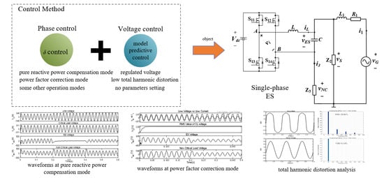
  • Enrich the control means of the ES;
  • Enable the circuit to operate in different power modes;
  • Model predictive control is used instead of the traditional controller to avoid the trouble of the controller parameter setting in the traditional system control;
  • Compared with the existing methods, the CL voltage distortion degree during line voltage distortion is further reduced.
The organization of the paper is as follows. Section 2 introduces the operating principles of the single-phase ES with the help of δ control. In Section 3, system modeling and design processes of MPC are provided. In Section 4, two controllers based on the same δ control, one is MPC and the other one is PR and P, are investigated as simulation cases to reveal better performances, such as harmonic suppression functions of MPC, and a brief discussion is given. Finally, the conclusions are drawn in Section 5.

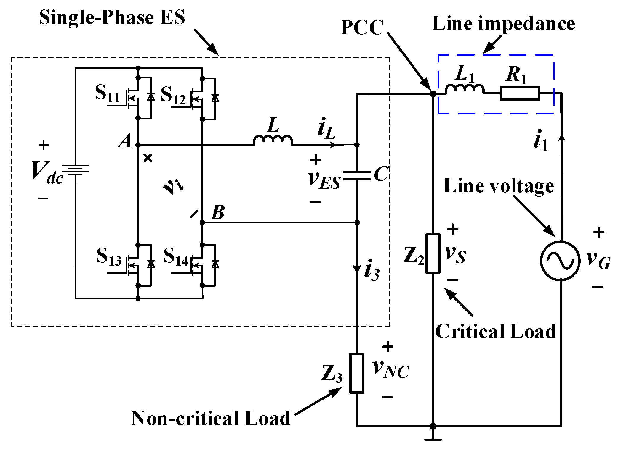
2. Operating Principles of Single-Phase ES

2.1. Topology of Existing Single-Phase ES

The existing single-phase ES circuit structure applied in the power system is shown in Figure 1. In this figure, the single-phase ES is in the dashed line, including a single-phase VSI and an LC filter. Z2 is the CL with limited operating voltage range and Z3 is the non-critical load (NCL) with wide operating voltage range. A smart load (SL) formed by a single-phase ES in series with Z3 is parallel to Z2. vG represents the voltage at the injection point of RES, R1 denotes line resistance, and L1 denotes line inductance. The series combination of vG and line impedance is connected to CL and SL. vS represents the voltage of the point of common coupling (PCC), which can be obtained by subtracting the vector vG from the voltage drop of the line impedance. As described in [7,8], the ES is a DC-AC conversion device that simultaneously transfers fluctuations of CL to NCLs.

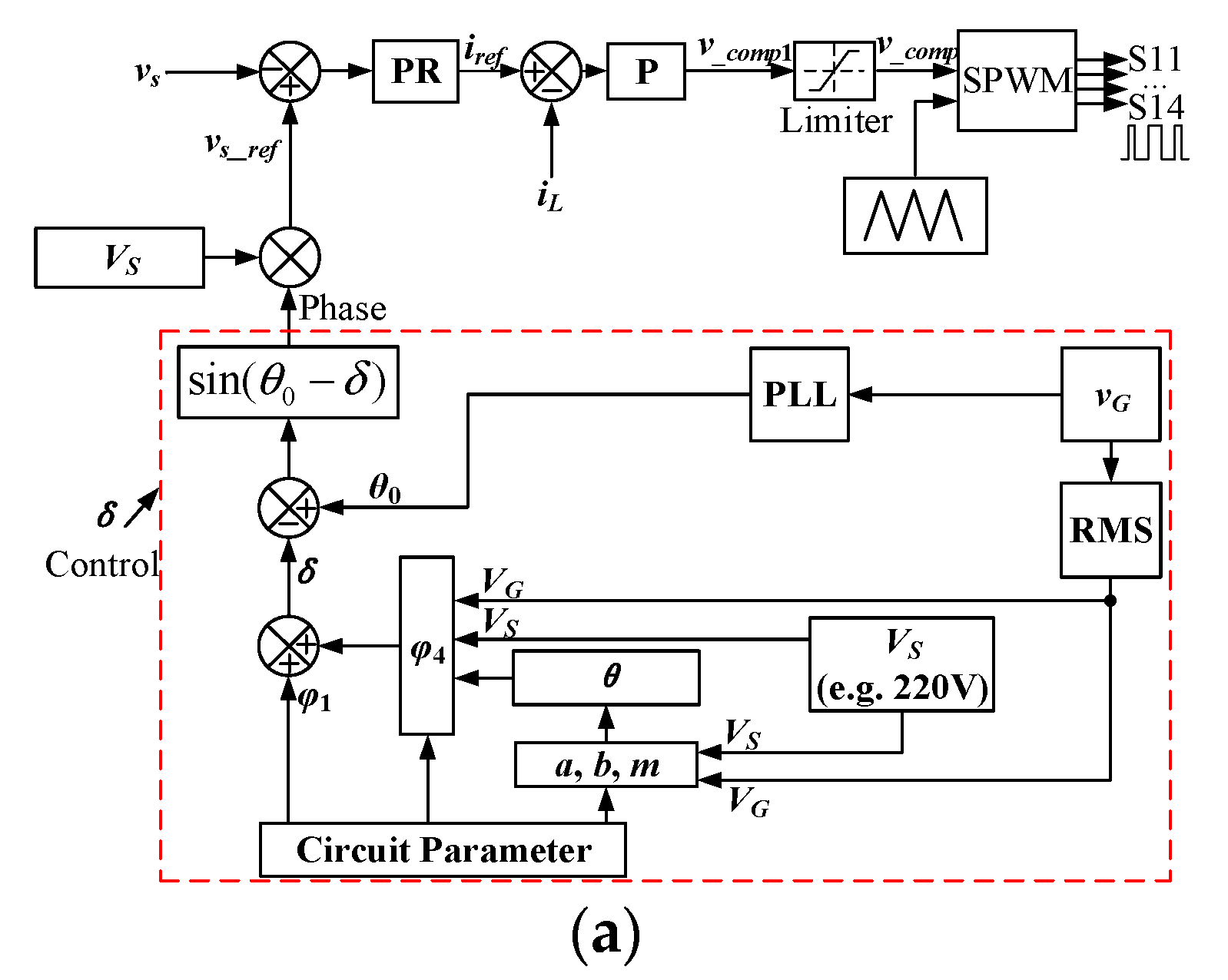
2.2. Existing δ Control

Figure 2a depicts an existing single-phase ES control diagram, which is referenced from [5]. As shown in the figure, the control diagram is designed with double loop control. The outer loop uses a PR regulator to control the CL voltage. The inner inductor-current loop is controlled by a P regulator. The reference value of the CL voltage vs_ref needs to be input in the PR regulator, whose instantaneous phase of the sinusoidal reference needs to be calculated by the δ control algorithm. The calculation process is also shown in the figure, which is based on a vector diagram, as shown in Figure 2b, which represents a certain operating mode of the ES, such as inductive mode. Once the CL voltage is regulated as expected, two control objectives of the ES can be achieved together.
The details of the PR and P controllers in Figure 2a are as follows. vS is the transient CL voltage. Its reference is a predefined sinusoidal signal. The magnitude is given manually and the phase is calculated in advance based on the certain operating mode by δ control. The residual is then fed to the PR controller to generate the inductor-current reference signal of the inner loop, that is iref. The current error between the sensed inductor current iL and iref is fed to the P regulator to generate the modulation signal v_comp via a limiter. At last, the drive signals of switches are generated by the SPWM generator. It is obvious to see that δ calculation in the dashed line is the key point which influences the input signal reference and the operation modes directly.
Figure 2b shows the vector diagram of the ES circuitry of Figure 1 when the circuit operates in the inductive mode in which CL voltage is greater than its rated value. The calculation details of δ are elaborated in [5]. Other operating modes of the ES circuitry can be illustrated similarly. One remark is that this method is implemented on the assumption that the impedance of the transmission line has been calculated, and the way of impedance calculation can be found in [21].

2.3. Disadvantages of Existing δ Control

Under ideal power grid conditions, the existing control strategies can effectively control the single-phase ES. However, when vG distorts to some extent based on PR and P controllers, the total harmonic distortion (THD) value of the CL voltage will be high and sometimes beyond tolerable limits. Although the THD value can be improved by debugging parameters of the controllers, it is very troublesome to set the parameters in practical application and often cannot achieve the ideal condition. For instance, kp of the PR controller cannot be more than 3, otherwise it will have a suppression effect beyond the specific frequency. An example occurs when the parameters of the PR regulator are set to 2 (kp) and 20 (kr), meanwhile the parameter for the P regulator is chosen as 0.5. As shown in Figure 2c, while THD of vG is 22.91%, that of the CL voltage will be up to 4.48%. It is still necessary and has potential to find a better controller.

3. Model Predictive Control of Single-Phase ES

3.1. The Proposed MPC for Single-Phase ES

In Figure 3, a new control method is proposed using MPC to replace the existing P and PR regulators. It is observed that the proposed control is also based on δ control. The differences between Figure 3 and Figure 2a are the different signal generators outside the dashed lines. The effectiveness and comparison will be illustrated in the next sections. Since MPC is related to a specific model, establishing the mathematical model of the system is the first task.

3.2. System Modeling of Single-Phase ES

As mentioned in [7], ignoring the DC bus dynamics, the linear time-invariant equations can be set up from Figure 1, by applying Kirhhoff’s Current Law (KCL):
i 3 = C d v E S d t i L ,
i 3 R 3 + v E S R 2 + i 3 = i 1 ,
Applying Kirhhoff’s Voltage Law (KVL) to Figure 1 also yields:
L d i L d t + v E S = v i ,
L 1 d i 1 d t + i 1 R 1 + v E S + i 3 R 3 = v G ,
v S = v E S + i 3 R 3 ,
v S = v G i 1 R 1 L 1 d i 1 d t ,
where i3 is the current through NCL, vES represents the capacitor voltage, iL is the current of inductor L, i1 is the line current through vG, vi is the output voltage of the full bridge inverter, and vS is the CL voltage.
Solving (1) to (4) yields:
{ d i L d t =   v E S L   +   v i L d v E S d t = i L C     v E S C ( R 2   +   R 3 )   +   R 2 i 1 C ( R 2   +   R 3 ) d i 1 d t = R 2 v E S L 1 ( R 2   +   R 3 ) ( R 1 R 2   +   R 2 R 3   +   R 3 R 1 ) i 1 L 1 ( R 2   +   R 3 ) + v G L 1 .
Solving (7) to (6) yields:
v S = R 2 R 2 + R 3 v E S + R 2 R 3 R 2 + R 3 i 1 .

3.3. Discrete-Ttime State Space Model

In order to implement the MPC algorithm into DSP, the discrete-time state space model is obtained using first-order approximation [19]. The differential forms of the state variables can be written as:
{ d i L d t = i L ( k   +   1 )     i L ( k ) T S d v E S d t = v E S ( k   +   1 )     v E S ( k ) T S d i 1 d t = i 1 ( k   +   1 )     i 1 ( k ) T S ,
where TS denotes the switching period. Substituting (9) into (7) yields:
i L ( k + 1 ) = i L ( k ) T S L v E S ( k + 1 ) + T S L v i ,
i 1 ( k + 1 ) = i 1 ( k ) m 1 T S R 2 m 1 L ( R 2 + R 3 ) v E S ( k + 1 ) + 1 m 1 L 1 v G ,
v E S ( k + 1 ) = v E S ( k ) m 2 T S + i L ( k ) m 2 C + T S v i m 2 L C + R 2 i 1 ( k + 1 ) m 2 C ( R 2 + R 3 ) ,
where,
m 1 = 1 T S + R 1 R 2 + R 2 R 3 + R 3 R 1 L 1 ( R 2 + R 3 ) ,
m 2 = 1 T S + 1 C ( R 2 + R 3 ) + T S L C .
Substituting (11) into (12) yields
v E S ( k + 1 ) = m 4 v E S ( k ) + m 5 i L ( k ) + m 6 i 1 ( k ) + m 7 v i + m 8 v G ,
where,
{ m 3 = 1 + R 2 2 m 1 m 2 L 1 C ( R 2   +   R 3 ) 2 m 4 = 1 m 2 m 3 T S m 5 = 1 m 2 m 3 C m 6 = R 2 m 1 m 2 m 3 C T S ( R 2   +   R 3 ) m 7 = T S m 2 m 3 L C m 8 = R 2 m 1 m 2 m 3 L 1 C ( R 2   +   R 3 ) .
Substituting (11) and (15) into (8) yields predicted the CL voltage vS(k + 1), which can be rewritten as:
v S ( k + 1 ) = R 2 R 2 + R 3 v E S ( k + 1 ) + R 2 R 3 R 2 + R 3 i 1 ( k + 1 )
The cost function can be defined as:
J = | v S ( k + 1 ) v S _ r e f | .

3.4. VSI Modeling and Switching State Selection

In Figure 1, the switching functions of the single-phase VSI are defined SA and SB, which are expressed as:
S A = { 1 @ S 11 = 1 & S 13 = 0 1 @ S 11 = 0 & S 13 = 1 ,
S B = { 1 @ S 12 = 1 & S 14 = 0 1 @ S 12 = 0 & S 14 = 1 .
The output voltage of VSI can be expressed as:
v i = ( S A S B ) V d c 2 .
In the proposed prediction algorithm, all of the four switching states in (19) and (20) will be checked to get four different voltage predictions. The switching state under which J in (18) reaches its minimum value will be selected during the next sampling instant. There are two cases where SA minus SB is equal to 0. Both cases are the same, which means that no current is passing through the full bridge. Two switch states can be selected evenly.

4. Simulation and Discussion

To verify the aforementioned method, simulations are conducted under the environment of MATLAB/Simulink and based on the parameters shown in Table 1. Since the load type only affects the calculation of δ, the resistive load can be used for all the loads to simplify the verification. Two compensation modes are selected as examples, of which the one is pure reactive power compensation mode and the other is PFC mode. There are two control indicators. The first is to ensure that the voltage of CL is stable at 220 V, and the second is to require the circuit to work in the predetermined operation mode.

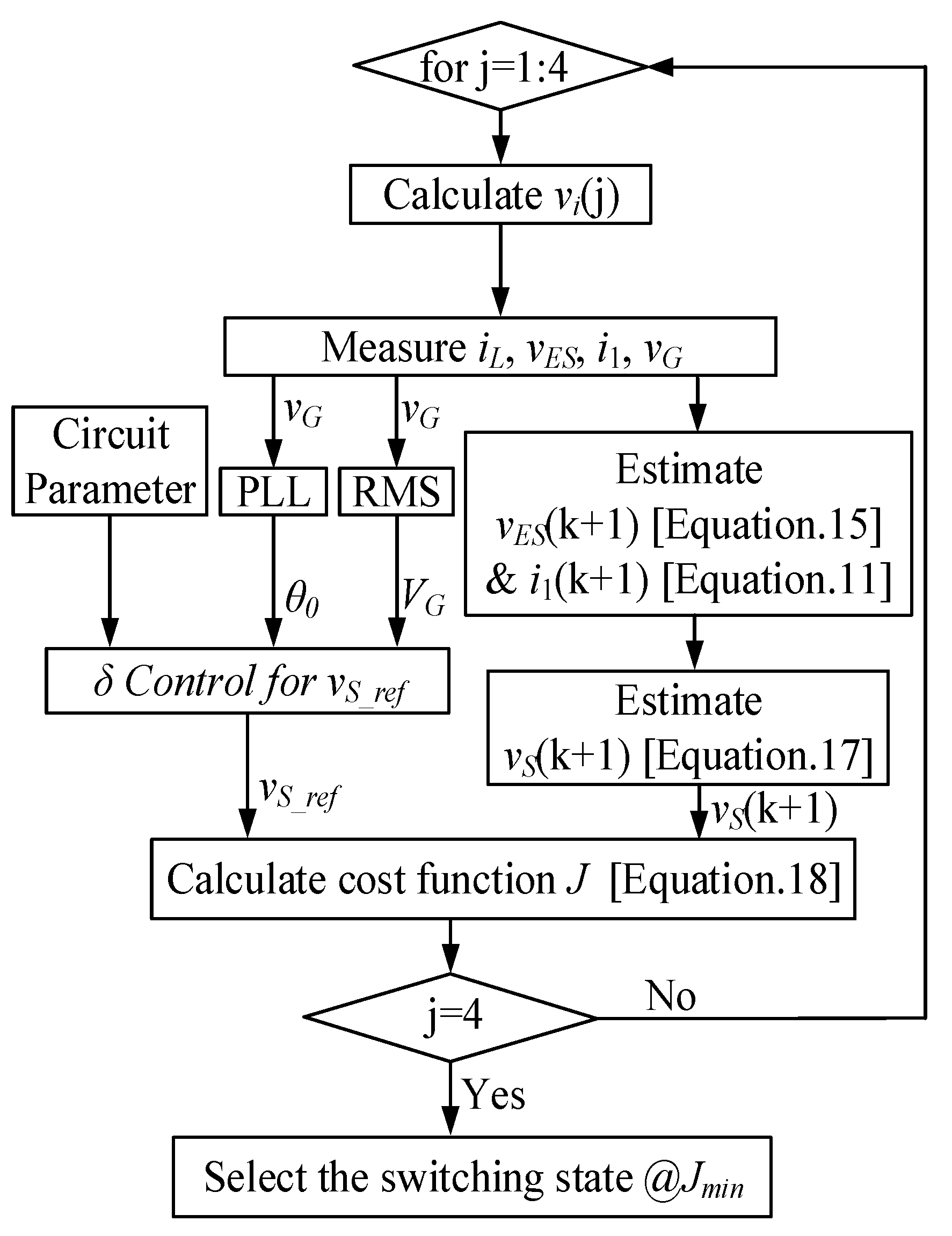
4.1. Flowchart of MPC and δ Control

MPC and δ control are realized by programming in the block of MATLAB (MathWorks, Natick, MA, USA) from its official website. Here the Matlab Function is a built-in module) Function. The specific flowchart is shown in Figure 4 which can be summarized as follows.
  • Measure grid voltage vG, grid current i1, inductor current iL, and ES voltage vES;
  • Predict vS based on the predicted ES voltage and predicted grid current;
  • Calculate the reference of vS based on the required circuit parameters and instantaneous phase and root-mean-square value of vG;
  • Calculate the cost function J considering all the four switching states;
  • Select the switching state that minimizes the cost function J and apply it to the inverter.

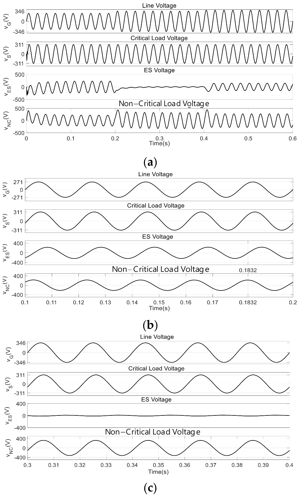
4.2. Pure Reactive Power Compensation Mode

In this part, the circuit works in the mode of pure reactive power compensation, where the phase difference between the voltage and current of the ES should be 90 degrees. In order to verify the robustness of the proposed method, the simulation is divided into two parts. One is when the power grid is under the ideal conditions and the other is when the power grid is distorted.

4.2.1. Ideal Grid Condition

When the power grid is under ideal conditions, there is no distortion on vG. The whole simulation is carried out under ideal power grid conditions. It is divided into three parts according to the time period, and each part corresponds to different impedance characteristics of the power grid. According to [7], when VG is set to 192 V, 244.5 V, and 267 V, capacitance, resistance, and inductance characteristic modes of the power grid can be simulated, respectively. The simulation waveforms of the full-time range is shown in Figure 5a, which includes four channels representing line voltage VG, critical load voltage VS, ES voltage VES, and non-critical load voltage VNC (which can reflects the current phase angle of ES), respectively.
Figure 5b–d is detailed subgraphs of the three time periods, respectively. When the grid is in a capacitive mode (line voltage is set to 192 V), it can be observed that the phase angle of the ES current leads the voltage 90 degrees at 0.1832 s. In Figure 5c, when the line voltage is 244.5 V, the circuit works in a resistive mode, and therefore VES is almost zero and the voltage of critical load is almost equal to that of the non-critical load. Finally, in Figure 5d, when line voltage is set to 267 V, the circuit works in a inductive mode and the phase angle of the ES current lags that of the ES voltage by 90 degrees at 0.5873 s. As can been seen from Figure 5b–d, VS is well controlled to be sinusoidal and there is little fluctuation on RMS values. Figure 5e shows the minimum value of cost function J during the simulation. It can be observed that the tracking error of the CL voltage is small.
The results above prove that the control method combining the proposed MPC and δ control can effectively regulate the ES voltage and achieve pure reactive power compensation under ideal grid conditions.

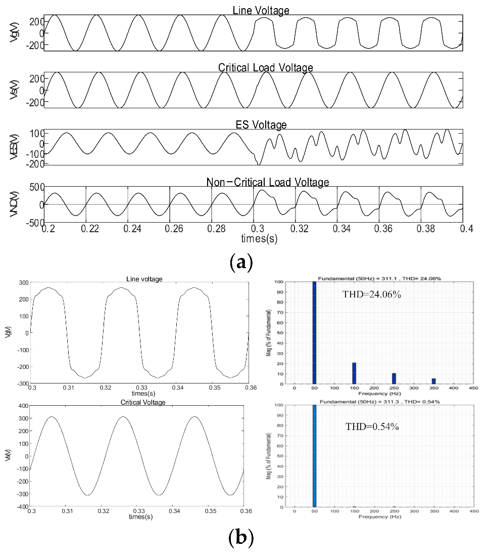
4.2.2. Grid Voltage Distorted
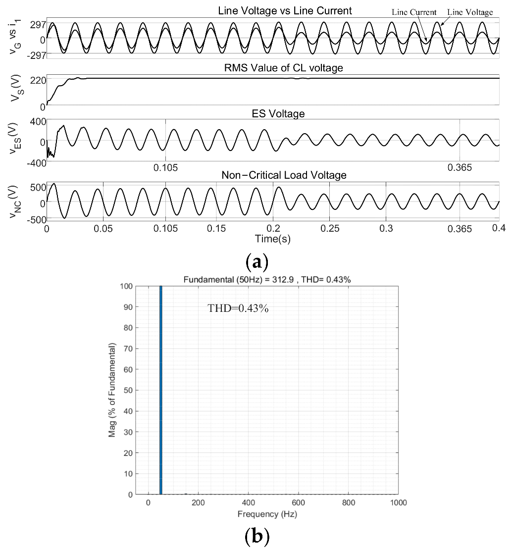
In this simulation, the disturbance is added to the line voltage, and other conditions are the same as in the previous simulation. The specific changes are as follows. From 0 to 0.3 s, the line voltage is given as a standard 220 V sinusoidal signal without any distortion. From 0.3 s to 0.6 s, the 3rd, 5th, 7th, and 9th harmonic components are added to the fundamental wave, and the RMS of these harmonic components are 44 V, 22 V, 11 V, 5.5 V, respectively. As a result, the THD value of line voltage is up to 24.06%, which is the same as that in Figure 2c.
Figure 6a shows the dynamic waveforms of the voltage change before and after line voltage distortion, where the circuit remains in capacitive mode the entire time. Before 0.3 s, the circuit works stably. However, after 0.3 s, it is obvious that when distortion occurs with line voltage, the voltages of the ES and non-critical load have corresponding distortion. While the critical load voltage has hardly changed, which indicates that ES successfully transfers the fluctuation of CL to NCL. What is more, in [5], using PR and P controllers, the THD of the CL voltage is as high as 4.48%, as shown in Figure 2c. Additionally, in another method combining dead-beat control and state observer, THD is reduced to 1.54%, but there is still room for progress. In Figure 6b, the THD value of the CL voltage is reduced to 0.54%, which is far smaller than that of the existing control method mentioned previously.

4.3. PFC Mode

In this part, performance of the proposed control method is rechecked. In order to ensure that the proposed method can be applied to a variety of working modes, this simulation will be in PFC mode, and other simulation conditions will be the same as before. The switching of operating modes depends on the difference of δ calculation, which is explained in [7] in detail. The simulation process is divided into two time intervals as shown in Figure 7a. The difference is the change of the line voltage. In the first time interval (0~0.2 s), the line voltage is set to 210 V, and in the second time interval (0.2~0.4 s), the line voltage is increased to 220 V. To facilitate observation and comparison, the line voltage and line current are recorded together in the same channel. It can be clearly observed that the phase angles of the two are almost identical, having the same zero crossing points and changing direction, even when the line voltage changes. The waveforms in channel 2, 3, and 4 demonstrate the ability of the ES to stabilize the critical load voltage. It is worth noting that ES can only meet two control objectives at the same time, which means power compensation cannot be guaranteed while PFC is guaranteed. The phase angle between the ES voltage and current is not completely synchronized. As indicated in Figure 7a, at 0.105 s, the phase angle of the ES current leads that of the voltage for more than 90 degrees, reflecting that ES is providing active power. At 0.365 s, the phase angle of the ES current leads that of the voltage for less than 90 degrees, reflecting that the ES is absorbing active power.
In order to test the ability of the method to suppress harmonics in different modes, the distortion is added to the line voltage, as in the previous section. FFT analysis of the critical load voltage can obtain the result shown in Figure 7b. The total harmonic distortion is reduced to 0.43%, which is within the tolerable range.
The simulation results under the two different operating modes above fully demonstrate the feasibility of the proposed method and its effectiveness in harmonic suppression.

4.4. Discussion

The existing single-phase ES control method has been able to control the critical load voltage and monitor the compensation mode of the system. However, the main idea of this paper is to improve the harmonic suppression ability of the circuit, so that the power quality of the grid is improved. More importantly, the proposed control method is simpler in implementation and avoids the difficulty of controller parameter design. Additionally, to increase the control precision, it is necessary to raise the switching frequency.

5. Conclusions

Model predictive control is proposed to cooperate with the recent proposed δ control as a new control strategy for single-phase ESs. This is possibly the first attempt to add MPC and δ control together for ESs. System modeling is analyzed first to get differential forms of all the three state variables. The discrete-time state space model is obtained through first-order approximation. The CL voltage can be predicted by the prediction of the ES voltage and line current. Although the CL voltage can be predicted by mathematical deviations, it is still difficult to get the cost function since the ES and its typical application circuit belong to a multi-input and multi-output system and there are two multiple objectives at the same time. With the help of δ control, one critical control objective which indicates the operating function of the ES is simplified because this important information is contained in the calculated reference signal of the CL voltage. As a result, the cost function is obtained as the absolute value of the error between the predicted CL voltage and its reference. Once the cost function is minimized to a limited range, the CL voltage fluctuation is constrained to a minimal range, and the power compensation mode is automatically satisfied because of the δ calculation. Among all the compensation modes, the most important and commonly used modes named pure reactive power compensation mode and PFC mode are selected as examples and simulated to validate the proposed control strategy, revealing that both control objectives can be achieved with the proposed MPC and δ control. Finally, two core advantages of the proposed method are pointed out and verified: One is that the empirical selection of controller parameters is avoided by programming logic control. Another is to effectively eliminate the harmonic components of the CL voltage when the grid is distorted. The simulation results show that the total harmonic distortion on the critical load can be limited to about 0.5%.

Author Contributions

Conceptualization, Q.W. and H.D.; methodology, Q.W.; software, H.D.; validation, H.D. and Q.W.; formal analysis, Q.W.; investigation, S.Y.; resources, Q.W.; data curation, Q.W.; writing-original draft preparation, H.D. and Q.W.; writing–review and editing, Q.W.; visualization, S.Y.; supervision, Q.W. and G.B.; project administration, Q.W.; funding acquisition, Q.W. All authors have read and agreed to the published version of the manuscript.

Funding

This work was supported by the National Natural Science Foundation of China under projects 52177171 and 51877040.

Institutional Review Board Statement

Not applicable.

Informed Consent Statement

Not applicable.

Conflicts of Interest

The authors declare no conflict of interest.

References

  1. Cheng, M.; Zhu, Y. The state of the art of wind energy conversion systems and technologies: A review. Energy Convers. Manag. 2014, 88, 332–347. [Google Scholar] [CrossRef]
  2. Hu, H.; Shao, Y.; Tang, L.; Ma, J.; He, Z.; Gao, S. Overview of harmonic and resonance in railway electrification systems. IEEE Trans. Ind. Appli. 2018, 54, 5227–5245. [Google Scholar] [CrossRef]
  3. Yang, T.; Mok, K.; Ho, S.; Tan, S.; Lee, C.; Hui, R. Use of integrated photovoltaic-electric spring system as a power balancer in power distribution networks. IEEE Trans. Power Electron. 2019, 34, 5312–5324. [Google Scholar] [CrossRef]
  4. Qiu, D.; Yuan, C.; Zhang, B.; Ke, M.; Chen, Y.; Xie, F. An improved electric spring topology based on LCL Filter. IEEE Trans. Power Electron. 2022, 37, 5984–5994. [Google Scholar] [CrossRef]
  5. Wang, Q.; Cheng, M.; Chen, Z.; Wang, Z. Steady-state analysis of electric springs with a novel δ control. IEEE Trans. Power Electron. 2015, 30, 7159–7169. [Google Scholar] [CrossRef]
  6. Mok, K.; Tan, S.; Hui, S. Decoupled power angle and voltage control of electric springs. IEEE Trans. Power Electron. 2016, 31, 1216–1229. [Google Scholar] [CrossRef]
  7. Tan, S.; Lee, C.; Hui, S. General steady-state analysis and control principle of electric springs with active and reactive power compensations. IEEE Trans. Power Electron. 2013, 28, 3958–3969. [Google Scholar] [CrossRef]
  8. Chen, T.; Liu, H.; Lee, C.; Hui, S. A generalized controller for electric-spring-based smart load with both active and reactive power compensation. IEEE Trans. Emerg. Sel. Topics Power Electron. 2020, 8, 1454–1465. [Google Scholar] [CrossRef]
  9. Zhao, H.; Zhao, J.; Zheng, Y.; Qiu, J.; Wen, F. A hybrid method for electric spring control based on data and knowledge integration. IEEE Trans. Smart Grid 2020, 11, 2303–2312. [Google Scholar] [CrossRef]
  10. Wang, Q.; Ding, Z.; Cheng, M.; Deng, F.; Buja, G. Direct power control of three-phase electric springs. IEEE Trans. Ind. Electron. 2022, 69, 13033–13044. [Google Scholar] [CrossRef]
  11. Wang, M.; Yan, S.; Tan, S.; Hui, S. Hybrid-DC electric springs for DC voltage regulation and harmonic cancellation in DC Microgrids. IEEE Trans. Power Electron. 2018, 33, 1167–1177. [Google Scholar] [CrossRef]
  12. Wang, M.; Mok, K.; Tan, S.; Hui, S. Multifunctional DC electric springs for improving voltage quality of DC grids. IEEE Trans. Smart Grid 2018, 9, 1552–1561. [Google Scholar] [CrossRef]
  13. Liang, L.; Yi, H.; Hou, Y.; Hill, D. An optimal placement model for electric springs in distribution networks. IEEE Trans. Smart Grid 2021, 12, 491–501. [Google Scholar] [CrossRef]
  14. Chen, J.; Yan, S.; Yang, T.; Tan, S.; Hui, S. Practical evaluation of droop and consensus control of distributed electric springs for both voltage and frequency regulation in microgrid. IEEE Trans. Power Electron. 2019, 34, 6947–6959. [Google Scholar] [CrossRef]
  15. Mohammadali, N.; Jamshid, A.; Sasan, P. Hybrid stochastic/robust flexible and reliable scheduling of secure networked microgrids with electric springs and electric vehicles. Appl. Energy 2021, 300, 117395. [Google Scholar]
  16. Mohammadali, N.; Jamshid, A.; Sasan, P. Flexible operation of grid-connected microgrids using electric springs. IET Gener. Transm. Dis. 2019, 14, 254–264. [Google Scholar]
  17. Mohammadali, N.; Jamshid, A.; Taher, N.; Sasan, P.; Matti, L. Bi-level fuzzy stochastic-robust model for flexibility valorizing of renewable networked microgrids. Sustain. Energy Grids 2022, 31, 100684. [Google Scholar]
  18. Mohammadali, N.; Jamshid, A.; Sasan, P. Flexibility pricing of integrated unit of electric spring and EVs parking in microgrids. Energy 2022, 239, 122080. [Google Scholar]
  19. Wang, W.; Yan, L.; Zeng, X.; Fan, B.; Guerrero, J. Principle and design of a single-phase inverter based grounding system for neutral-to-ground voltage compensation in distribution networks. IEEE Trans. Ind. Electron. 2017, 64, 1204–1213. [Google Scholar] [CrossRef]
  20. Hu, Y.; Deng, Y.; Liu, Q.; He, X. Asymmetry three-level grid-connected current hysteresis control with varying bus voltage and virtual oversample method. IEEE Trans. Power Electron. 2014, 29, 3214–3222. [Google Scholar] [CrossRef]
  21. Pavlou, K.; Vasiladiotis, M.; Manias, S. Constrained model predictive control strategy for single-phase switch-mode rectifiers. IET Power Electron. 2012, 5, 31–40. [Google Scholar] [CrossRef]
  22. Gong, Z.; Wu, X.; Dai, P.; Zhu, R. Modulated model predictive control for MMC-based active front-end rectifiers under unbalanced grid conditions. IEEE Trans. Ind. Electron. 2019, 66, 2398–2409. [Google Scholar] [CrossRef]
  23. Xie, C.; Zhao, X.; Li, K.; Zou, J.; Guerrero, J. Multirate resonant controllers for grid-connected inverters with harmonic compensation function. IEEE Trans. Ind. Electron. 2019, 66, 8981–8991. [Google Scholar] [CrossRef] [Green Version]
Figure 1. The existing topology and typical application circuit of the single-phase ES.
Energies 15 06654 g001
Figure 2. Existing control strategy. (a) Control diagram referenced from [5], (b) Vector diagram of δ control setting inductive mode, (c) Total harmonic distortion analysis of line voltage and CL voltage under distorted conditions.
Energies 15 06654 g002aEnergies 15 06654 g002b
Figure 3. The proposed MPC based on δ control.
Energies 15 06654 g003
Figure 4. Program flowchart of MPC and δ control.
Energies 15 06654 g004
Figure 5. Simulation waveforms based on the proposed control method under the mode of pure reactive power compensation without grid distortion. (a) Full time range of waveforms under various grid impedance modes. (b) Capacitive mode @VG = 192 V. (c) Resistive mode @VG = 244.5 V. (d) Inductive mode @VG = 267 V. (e) Minimum values of cost function J.
Energies 15 06654 g005aEnergies 15 06654 g005b
Figure 6. Simulation waveforms based on the proposed control method under the mode of pure reactive power compensation with grid distortion. (a) Comparison of the waveforms between ideal grid condition and distorted condition. (b) THD analysis of line voltage and critical load voltage under distorted grid condition.
Energies 15 06654 g006
Figure 7. Simulation waveforms at PFC mode. (a) Four channels of waveforms. (b) THD analysis of critical load voltage.
Energies 15 06654 g007
Table 1. Parameters for simulation.
ParametersValues
Regulated mains voltage (VS)220 V
DC bus voltage (Vdc)400 V
Line resistance (R1)0.1 Ω
Line inductance (L1)2.4 mH
Critical load (R2)43.5 Ω
Non-critical load (R3)2.2 Ω
Inductance of low-pass filter (L)3 mH
Capacitance of low-pass filter (C)50 µF
Switching frequency (fs)20 kHz
Publisher’s Note: MDPI stays neutral with regard to jurisdictional claims in published maps and institutional affiliations.

