1. Introduction
As electricity generation from renewable energy sources has increased, so has the use of energy storage systems. Specific energy, specific power, lifetime, and reliability are among the most important criteria considered when selecting a storage system. There are various electrical energy storage systems, among which the systems of lithium-ion batteries stand out due to their high energy density and acceptable lifetime [
1]. The safe, reliable, and efficient operation of batteries requires a battery management system (BMS) that monitors, diagnoses, and keeps the battery in operation. The main parameters monitored and diagnosed by the BMS are state of charge (
SoC), state of health (SoH), and battery temperature.
There are different definitions of battery capacity and
SoC. According to [
2],
SoC is defined as the ratio of the charge difference of a fully charged battery
CN and the amount of discharged charge
Qb with respect to the amount of charge of a fully charged battery:
where:
CN—charge of the fully charged battery, [Ah],
Qb—amount of discharge charge of battery, [Ah].
According to this definition, a full state of charge is reached when the battery current does not change within 2 h at constant charge voltage and temperature. Estimating the
SoC is not a simple task because the
SoC depends on the capacity, temperature, and internal resistance of the battery. It is desirable to keep
SoC of batteries within reasonable and safe limits such as 20% ≤
SoC% ≤ 95% [
3].
The
SoC of a battery cannot be measured directly, but it can be estimated using various methods [
4]. Two typical
SoC evaluation methods are the open circuit voltage (OCV) method and the coulomb method, i.e., the ampere-hour or coulomb counting method. The OCV method estimates
SoC indirectly by measuring the open-circuit voltage of the battery and using tables with a predetermined
SoC–OCV relationship. Despite its reliability, this method is not practical in online applications because the battery must be relaxed for a period of time for the open-circuit voltage to reach a steady state. This method is also not suitable for batteries where the open-circuit voltage changes little with changes in the state of charge (flat OCV curve) [
5,
6]. The coulomb counting method is easy to implement due to its low computational cost, and it is based on numerical integration of the current over time. However, this method requires knowledge of the initial state of charge and is sensitive to the accuracy of the sensor measurements. Additionally, possible sources of error in this method are the reduction of capacity over time and self-discharge [
7]. The internal resistance of the battery can also be used to estimate the
SoC. However, the irregular correlation between the internal resistance and
SoC is not suitable for the reliable estimation of
SoC [
8].
In addition to the previously mentioned
SoC evaluation methods, there are also methods that use algorithms based on the battery model. Electrochemical models (EM) are commonly used for
SoC estimation [
9,
10]. EM use partial differential equations to model the physics of the battery. To achieve a good balance between computational cost and accuracy, a low-complexity
SoC prediction method uses a simplified electrochemical model. The battery model can be used to calculate the battery voltage based on the known input current, temperature, and
SoC. Assuming that the battery model is correct, the calculated voltage would be equal to the measured voltage. Any discrepancy between the battery voltage calculated by the model and the measured voltage can be used to correct the
SoC at any point during calculation over time. In general, model-based methods such as the Kalman filter (KF), extended Kalman filter (EKF) [
11,
12], unscented Kalman filter (UKF) [
13], H infinite filter (H∞), sliding mode observer [
14], and others [
15,
16,
17] are insensitive to the value of the initial SoC due to the internal closed-loop structure and have high accuracy and excellent stability. However, an accurate battery model is required for accurate
SoC estimation since it is not possible to correct for modeling errors. Several other variants of the Kalman filter, e.g., sigma-point KF [
18], adaptive KF [
19], and derivative KF [
20], have also been used for
SoC battery estimation. However, further improvements to the algorithm lead to increased computational costs and implementation difficulties.
With the development of computers and artificial intelligence, intelligent algorithms such as support vector machine (SVM), fuzzy logic, and neural networks (NN) are increasingly used in
SoC evaluation. Without any information about the internal structure of the battery and the initial
SoC, these algorithms explore the relationship between the
SoC and measured variables such as battery voltage, current, and temperature according to the learning data [
21,
22,
23,
24,
25,
26]. However, the algorithms require a large memory to store the amount of data required for learning, which consequently burdens the entire system and results in long-term procedures and difficulties in implementation.
This paper describes a method for estimating the SoC based on the battery model and the relationship between the SoC and the dynamic response of the battery, i.e., the battery transfer function. It is assumed that the voltage response function to the current pulse is a nonlinear function of the SoC. By determining the transfer function of the voltage response to the current pulse at a particular point of the SoC, the parameters of the transfer function that depend on the SoC are obtained. The parameters of the transfer function can be considered as the coordinates of the hyperspace point for the corresponding SoC. In the learning phase of this method, a map was created to establish a link between the SoC and the corresponding transfer functions. The algorithm of the method starts with the online measurement of the voltage response of the battery to the corresponding current pulse and proceeds with the calculation of the parameters of the transfer function. The parameters of the transfer function for the unknown SoC form a new point of hyperspace from which the SoC of the battery is determined by interpolation from the Euclidean distance to the nearest points. The application of the method is illustrated by the SoC assessment of a high-capacity lithium-nickel-manganese-cobalt-oxide (LiNiCoMnO2) battery cell.
The novelty of the method is the estimation of the SoC based on the position in hyperspace of the point defined by the parameters of the transfer function and the determination of the parameters of the function by optimization from the time response of the battery voltage to the current pulse. The use of the optimization method to determine the parameters of the transfer function ensures insensitivity to measurement noise and is not very computationally demanding. The method is suitable for determining the SoC when the initial SoC is not known and has the potential for application to various battery chemistries.
What is special about this method is that it does not require a permanent measurement of the voltage and current at the battery but only the response of the voltage to a current pulse of about 3 s duration. This is especially important when the algorithm is not applied in the battery BMS but in a charging station for light electric vehicle batteries, which have no communication between the vehicle battery BMS and the station.
Methods based on Kalman filters require constant measurement of voltage and current and execution of an algorithm with a specific sampling time, making them suitable for use in BMSs where the BMS computer continuously executes algorithms for voltage monitoring and balancing, battery protection, and state of charge estimation. The algorithm described in this paper does not require the entire algorithm to be executed in real time.
The battery charging station for light electric vehicles can use its own converter to generate a current pulse, record the battery’s current and voltage signals, and send the recorded information packet to the monitoring computer in the station. After that, the converter is free to perform the battery charging function. A monitoring computer, which has no time-critical control functions, can perform the battery SoC estimation. In this way, the real-time converter controller is not burdened with complex mathematical estimation functions, while the data transmission to the monitoring computer is not time-critical because it is not part of the control loop.
The effectiveness of the proposed method was tested by simulation and experiments. In the second chapter of the paper, the used model of the lithium-ion battery is described; thus, the form of the transfer function is determined. The third chapter describes the principle of the new SoC estimation method. The fourth chapter describes the algorithm used in the learning phase, i.e., the formation of the reference base of SoCs and associated transfer functions, the laboratory setup used, and the results of the learning process. In the fifth chapter, the results of the determination of the unknown SoC using the proposed method are presented, followed by the conclusion.
2. Lithium-Ion Battery
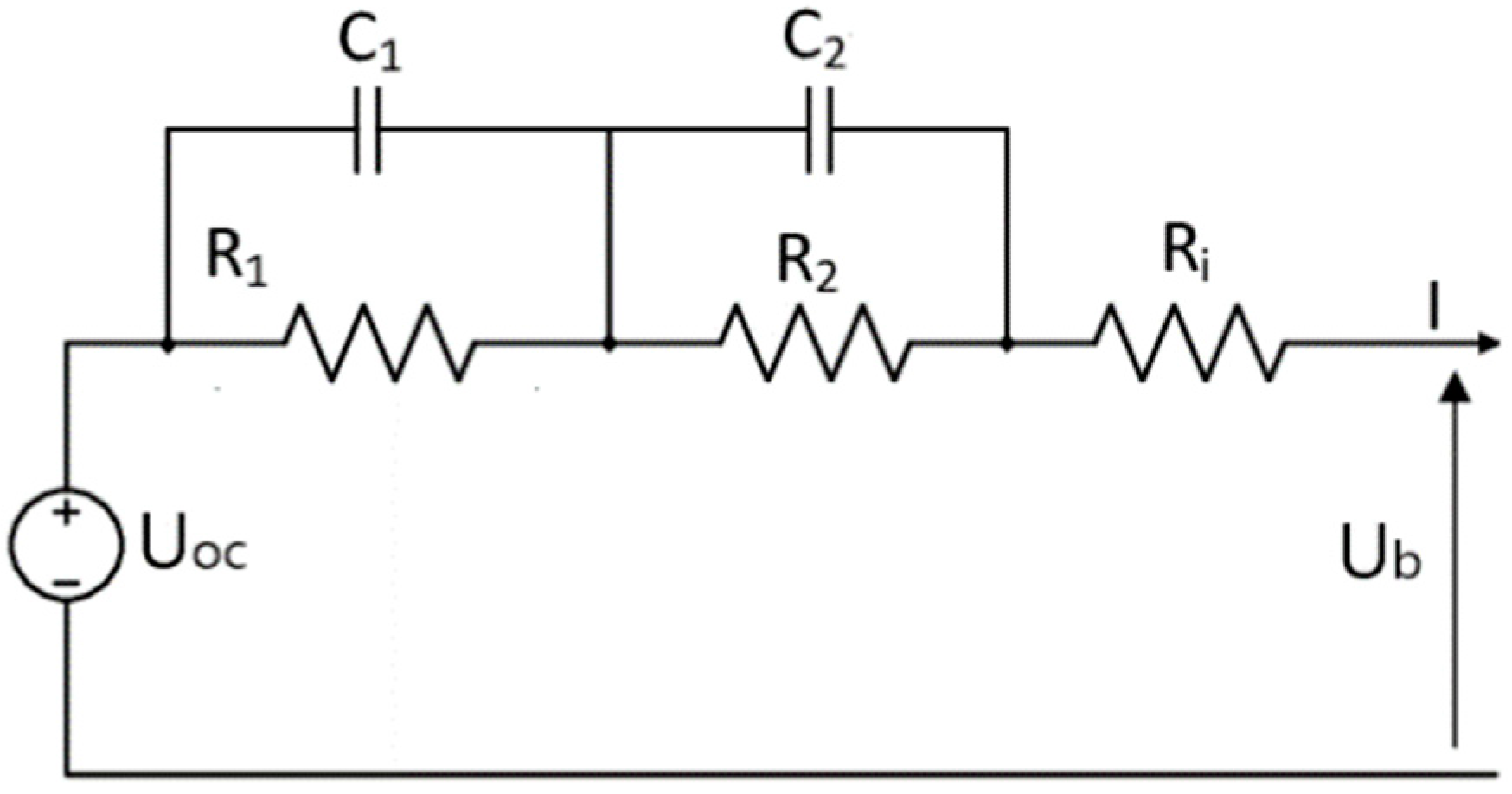
Among several electrical models of the battery, to evaluate the SoC, the equivalent circuit model (ECM) is used in this paper. The reasons for using this model are the good balance between accuracy and simplicity of the model. A basic ECM consists of an ideal voltage source, an internal resistance, and an RC circuit that represents the dynamic characteristics of the battery. The reason for the dynamic behavior of batteries is the polarization and diffusion between the battery electrodes.
However, to reliably determine the
SoC of the battery, it is necessary to extend the basic ECM with another RC circuit [
27]. The electrolyte inside the battery separates the battery’s electrodes, prevents short circuit, and allows ion flow between the electrodes. The properties of the electrolyte degrade over time, so the electrolyte particles eventually bind to the anode and form a second layer called the solid electrolyte interphase (SEI). As the battery ages, the impact of SEI on battery performance and dynamic behavior becomes more apparent. The basic ECM is extended by an additional RC circuit that models this influence (see
Figure 1). The time constant
R1C1 influences the transfer function of the extended ECM model; however, it was not investigated how this constant, by itself, affects the
SoC. This influence will be determined in the continuation of the research.
The voltage changes as a function of the current change at the operating point determined by the
SoC, and the voltage
Uoc for the ECM from
Figure 1 is determined by a second-order transfer function:
where:
K is the gain of the transfer function.
bi ∀ i = 0,…2—nominator parameters of the transfer function.
ai ∀ i = 0,…2—denominator parameters of the transfer function.
The battery voltage in the Laplace domain is determined by the expression:
where:
G(s) is the battery transfer function.
i(s) is the battery current in the Laplace domain [A].
u(s) is the battery voltage in the Laplace domain [V].
The transfer function (2) contains two zeros and two poles. However, the non-dominant zero and the non-dominant pole have less influence on the response and are very sensitive to measurement noise in the estimation. For this purpose, the estimation requires an equivalent transfer function
Ge(
s) containing one zero and two poles of the form:
Estimation determines the parameters of the transfer function that give the response closest to the measured one.
4. Learning Process
During the learning phase, measurements were taken for nine known SoCs, starting with an empty battery and ending with a full battery in 12.5% increments. To verify battery capacity, the battery was first discharged to the cutoff voltage and then charged to the allowable voltage using a constant current/constant voltage method with a charge current equal to 50% of the nominal charge current. The energy delivered was measured using the ampere-counting method. When the charging current dropped to 5% of the nominal charging current, the charging process was complete. This method establishes a relationship between the SoC of the battery and the amount of energy stored. The learning process itself began by discharging the battery again and by measuring the voltage response to a small current pulse for each desired point of the SoC to establish a table of reference values. For each reference point, the corresponding transfer function and certain parameters to be used for recognition were estimated.
4.1. Learning Algorithm
The learning algorithm is shown in the flowchart in
Figure 2. Measurements of the voltage response to a small current pulse were made at the values of stored energy corresponding to the following
SoC (%) values: [0, 12.5, 25.0, 37.5, 50.0, 62.5, 75.0, 87.5, 100].
The measurement of stored energy to determine the reference point of charge was performed using the ampere-counting method.
At each of the reference points of the
SoC, the voltage response to a small current pulse was recorded. The recorded current and voltage signals were stored with the corresponding
SoC of the battery. The procedure for estimating the transfer function parameters for each
SoC was performed by optimizing the parameters of the model determined by Equations (4) and (5).The parameters were optimized using the Nelder–Mead simplex method implemented in MATLAB according to the minimum of the
ISE criterion defined by the equation:
where:
- -
u(t) is the measured battery voltage response signal to the current pulse.
- -
um(t) is the voltage response signal of the battery model to the measured current pulse signal.
- -
T is the duration of the simulation.
In the estimation, the calculation of the criteria was performed during the entire time of the signal measurement, i.e., until the battery voltage stabilizes after the current pulse drops to zero.
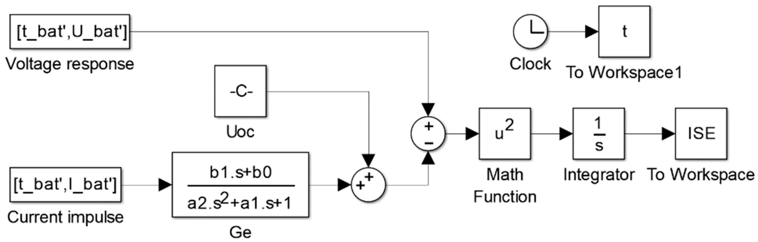
For this purpose, the MATLAB/Simulink battery voltage model is defined according to Equations (4) and (5), as shown in
Figure 3.
The transfer function of the dynamic part of the model in block Ge is described by Equation (4).
The parameter in block Uoc was determined before optimization as the average of the voltage signal before exposure to the current pulse, while the transfer function parameters were determined by optimization with the simplex method using the MATLAB fminsearch function from the optimization toolbox.
The vector of optimization parameters is defined by the expression:
The estimated transfer function is not limited to the aperiodic response of the voltage to the current pulse but also includes transient responses with overshoot.
From the estimated parameters of the transfer function
Ge, the parameters of the reference table are determined for each
SoC:
The dominant pole, i.e., the root of the denominator of the transfer function, is defined as the root of the denominator whose real part is closest to the origin. This was performed with MATLAB functions:
For each SoC measured in this way, a reference vector xR is determined, which can be represented by a point in four-dimensional Cartesian hyperspace.
To increase the accuracy of learning, it is possible to perform multiple measurements and estimations of transfer functions for the same SoC to obtain more associated vectors, i.e., points of the hyperspace for one SoC. In this case, the points form a cloud for the corresponding SoC, and the reference point to which the reference vector belongs is calculated as the centroid of the cloud points for each SoC.
The table of SoCs and associated vectors xR defines a piecewise linear function of the dependence of the SoC on the vector xR. Based on this, the determination of the unknown SoC can be carried out from the estimated values of the associated vector xR by finding two points with the smallest Euclidean distance from the point with the unknown SoC and determining the SoC by linear interpolation.
4.2. Experimental Setup for Learning
The experimental part of the research in the learning phase consisted of several charging and discharging cycles of the battery to determine the voltage profile, battery capacity, and the effects of charging power on battery temperature. The following equipment was used for the experiment:
Battery—SAMSUNG ICR 18,650—26 J M
Current sensor—HY 5-P,48,275, JP2
Current source—Magna—Power electronics, XR 50-40, 2 kW
Current pulse source—Iskra Power Supply (IPS), MA 4171, 1 A, 25 V
Laboratory Power Supply (LPS), PS—24,030, 0–40 V, 0.01–3 A
Electronic load—Hewlett Packard—6050a
Microcomputer for measurement and control—dSPACE—MicroLabBox
MATLAB/Simulink package on the PC computer
Battery specifications are given in
Table 1.
The equivalent electrical diagram of the laboratory setup is shown in
Figure 4, while the actual appearance of the laboratory setup is shown in
Figure 5.
A MATLAB script and real-time toolbox were used to control the dSpace microcomputer to synchronize controllable sources and measurements. Measurements and recording of measurement results were performed using dSPACE MicroLabBox. The sampling time was set to 100 μs to record the dynamic voltage response. All further data processing and parameter estimation were performed offline from the measured data in MATLAB/Simulink using the optimization toolbox, as described in the previous chapter.
4.3. Experimental Results of the Learning Phase
In the learning process, the battery for a given
SoC is excited by a current pulse, as shown in
Figure 6.
Nine SoC reference points were selected, evenly distributed in the range from 0 to 100%. Experiments have shown that nine points provide estimation accuracy with an error below 5%. For each state of charge (%) (0, 12.5, 25, 37.5, 50, 62.5, 75, 87.5, 100), multiple voltage responses are measured for identical current pulses. The transfer function parameters are calculated from each voltage response through an optimization process to obtain parameters for which the error in voltage estimation is minimal according to the ISE criterion.
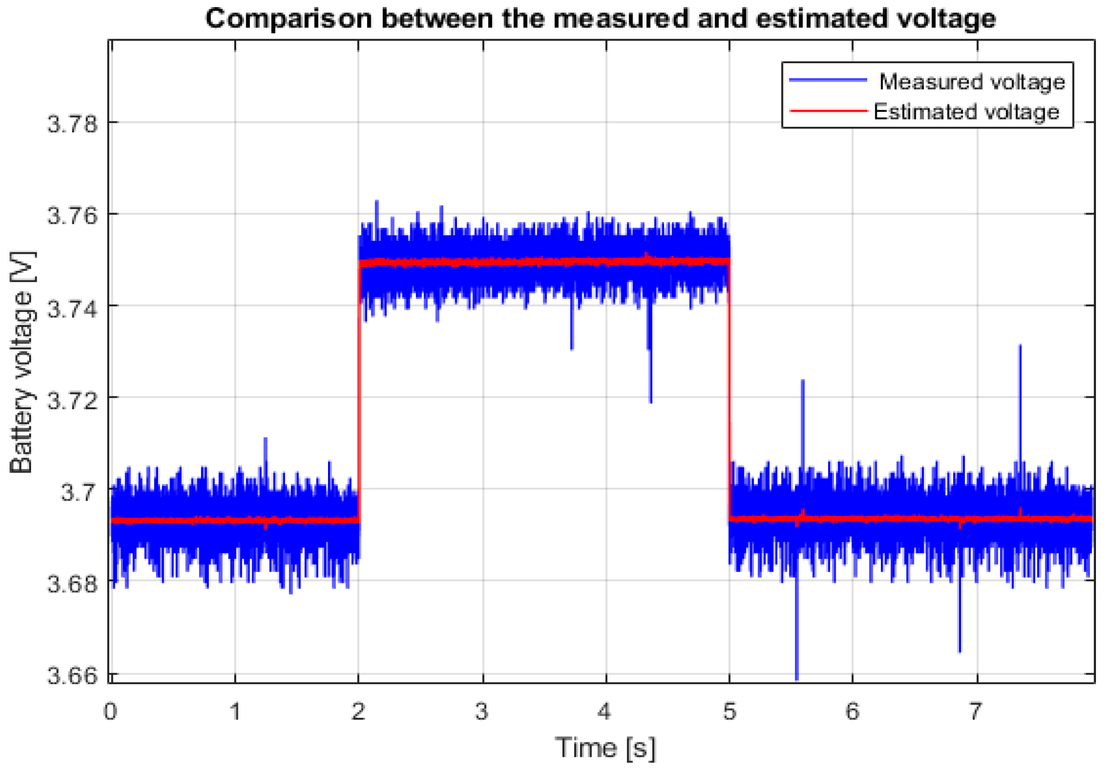
Figure 7 shows the measured voltage response to the current pulse and the Simulink model voltage with estimated parameters for the reference point
SoC = 50%. The difference between the signals is caused by noise. When this learning process is completed for all reference points, i.e.,
SoCs, the vector of transfer function coefficients
xR is stored in the reference table with the corresponding
SoC. This completes the learning phase. The matrix of learned values for the battery SAMSUNG ICR 18650–26J M is shown in
Table 2.
5. Estimation of the Unknown SoC
The process of
SoC estimation consists of three phases: (i) measurements of the voltage response to the current pulse at the studied
SoC, (ii) estimation of the vector
x = [
UOC K z p] in the same way as in the learning processes, and (iii) localization of the point in hyperspace determined by the test vector. The process of estimating the unknown
SoC is represented by the flowchart in the
Figure 8.
The evaluation of the SoC starts with the measurement of the voltage response of the battery to the current pulse with similar characteristics as in the learning phase.
The voltage response is used to calculate the UOC and the coefficients of the transfer function of the battery at the tested state of charge. The test vector xT is determined from the estimated parameters. The test vector xT determines a single point in hyperspace.
By determining its distance to the nearest reference points from the reference table, the corresponding SoC is estimated by interpolation.
The estimation of the corresponding SoC for the point determined by the vector xT is performed in two steps. First, the value of the parameter UOC is used to determine whether the vector belongs to one of the three ranges of SoC: [SoC < 25%, 25% ≤ SoC ≤75%, SoC > 75%].
In this way, the UOC has the greatest weight in determining the range. Then, the two points of the reference table closest to the point determined by the vector xT for the unknown SoC within the specified range are found.
For the localization of the test vector in hyperspace, the distance between two points is calculated based on the Euclidean norm according to the following equation:
where:
K is the system gain for measured and reference SoC.
p is the dominant pole of transfer function for measured and reference SoC.
UOC is the open-circuit battery voltage before current impulse for the measured and the reference SoC.
z is the zero of the transfer function for the measured and reference SoC.
The index test defines the membership of the parameter to the xT vector, and the ref index defines the parameter membership to the xR vector of the reference table.
In estimating the unknown SoC, a linear change in the SoC between two reference points is assumed, proportional to the distance between them.
Using the Euclidean norm, the two distances d1 and d2 corresponding to the two closest points of the reference table within the defined area of the SoC are determined. The distance d1 is the distance to the point with the lower SoC, while d2 is the distance to the point with the higher SoC.
The unknown
SoC represented by the vector
xT is determined by interpolation according to the equation:
where:
d1 is the distance from the point of the unknown SoC determined by the vector xT to the point SoClow.
d2 is the distance from the point of unknown SoC determined by the vector xT to the point SoChigh.
SoClow, SoChigh are the two points closest to the point of the unknown SoC determined by the xT vector.
5.1. Experimental Results of the SoC Estimation
In order to verify the success of the estimation algorithm, it is necessary to run it at points other than the reference points, since the error at the reference points is negligible. Since the state-of-charge estimation algorithm determines the closest
SoC reference points to the
SoC being estimated and performs linear interpolation based on the distance to the reference points, the largest error is expected to occur at the
SoC farthest from the reference points. The reference points define eight intermediate intervals, and the
SoCs farthest from the reference points are in the middle of the intervals. Therefore, to examine the worst-case estimation, eight test points located at the halves of the intervals defined by the reference points were selected. Thus, the test procedure for the
SoC (%) assessment algorithm includes eight points (6.25, 18.75, 31.25, 43.75, 56.25, 68.75, 81.25, 93.75). The evaluation results for eight test points are shown in
Table 3.
5.2. Analysis of the Results of the SoC Estimation
The first column of
Table 3 shows the actual
SoC obtained by applying the coulomb counting method, in percent. The second and third columns show between which two reference points the unknown
SoC is located. The fourth column shows the estimated
SoC value based on Equation (16). The last column shows the relative estimation error, which is calculated as the ratio of the difference between the actual
SoC value and the estimated
SoC value relative to the reference
SoC value. From
Table 3, it can be seen that each test point is accurately located, and the estimated
SoC value is very close to the actual value. The relative error is less than 2% in most cases. The only exception is 6.25%, where the relative error is almost 10%. Generally, at low states of charge, the nonlinearity of the battery is more pronounced, so the linear interpolation increases the estimation error. This will always be the case because with more pronounced nonlinearity, the interpolation method deviates more and more from the exact solution. Nonetheless, we can be certain that the battery is at low states of charge, which can be used to protect a battery from over-discharging. In this case, the estimated
SoC of 5.61% is below the true
SoC value of 6.25%.


