Identification of a Mathematical Model for the Transformation of Images for Stereo Correspondence Measurements of Mining Equipment

Abstract

The stereometry of the working units of mining machines is optimized at the design stage, in terms of selected criteria based on computer simulations of the mining process. The recovered bodies of cutting heads or drums used in manufacturing are regenerated in the overhaul process. Ensuring that their dimensions comply with the nominal ones is labor-intensive and raises production costs. However, deviations of these components from the nominal shape can make it difficult to position the pick holders (which can cause collisions) or make welding them impossible (which results from too large a distance between the pick holders’ base and the side surface of the working unit). This applies especially to robotic technologies. By utilizing automatic (online) measurements of the distribution of the actual distances of the pick holders’ bases from the side surface of the working unit (taken during their positioning using a robot), it is possible to correct their positions without changing the setting of the pick itself. This measurement can be carried out using the non-contact stereovision method. This paper presents a method of matching raster images obtained from a stereovision system installed on an experimental robotic station. The results are presented of the numerical research carried out to select a mathematical model of the geometric transformation of images, for ensuring the effectiveness of the developed method.

1. Introduction

Compliance of the final product with its design, especially in the mining industry where pick holders must be set on the working units of machines, is a necessary condition to ensure the effective course of the rock cutting process. The cutting heads (or drums) of mining machines are designed with the help of computer simulations, which mimic the conditions in which the roadheader or shearer will operate. The stereometry of the cutting head is then optimized for selected criteria, based on these computer simulations. The basic criteria for selecting a pick system include minimizing energy consumption, dynamic loads, and vibrations, and maximizing the cutting efficiency [1,2,3,4,5,6]. The recovered bodies of the cutting heads used in manufacturing are regenerated in the overhaul process, and ensuring that their dimensions comply with the nominal ones is not only labor-intensive, but also raises production costs. Therefore, dimensional deviations of the bodies of the cutting heads determine the need to control, in real-time during assembly, the positions of the pick holders to the side surface of the mining machine’s working unit. This especially applies to the use of robotic technology. It is possible to ensure the appropriate positioning of the pick holders so that they can be welded, thanks to the adaptive control of robots at the pick holders’ assembly station. This adaptive control enables the pick holder to be adjusted (without changing the pick tip) to obtain the best possible position of the base on the side surface of the working unit (which is to be welded), and ensures appropriate conditions for the implementation of a welded joint. In addition, online measurements of the distribution of the actual distances between the base of the pick holders and the side surface of the working unit enable the adjustment of the pick holders so that the handles do not collide with the body of the working unit.

Previous research confirms that the original method of automatic measurement of the distance between the pick-holder base and the side surface of the cutting head, performed with the use of a stereovision system, fulfilled its task according to metrological requirements [7]. Experiments of the developed method were carried out in the current study using the KUKA VisionTech stereovision system installed on a test stand, and conducted in the Robotics Laboratory of the Department of Mining Mechanization and Robotisation, in the Faculty of Mining, Safety Engineering, and Industrial Automation, at the Silesian University of Technology. The measurements consisted of determining the distribution of the distance between the measuring points on the cutting head’s body surface and the base surface of the positioned pick holder. These points were projected onto the side surface of the working unit of the mining machine using a laser, and the measurement was taken using the non-contact, stereophotogrammetric method. Image processing and the development of measurement results were carried out with the use of proprietary software written in Matlab, consisting of the following steps [8,9]:

• acquisition of measurement images (Figure 1a),
• image preprocessing (segmentation of measurement points) (Figure 1b),
• geometric transformation of the right image into the left image (Figure 1c),
• finding the stereo correspondence of measuring points (matching) (Figure 1d),
• discrete reconstruction of the shape of the working unit’s side surface where the pick holder is attached (Figure 1e).

The Image Processing Toolbox and Computer Vision Toolbox libraries were used in Matlab, and the functions available in these libraries were implemented in the software allowing the automatic identification of the position of the markers on the images of the cutting head’s side surface [10]. This work is a continuation of previous research and provides a solution to the problem of finding stereo correspondence of measurement points recorded in images. This stage is crucial for the correct reconstruction of measurement points in the spatial model and thereby the obtained measurement results [11,12].

Currently, commonly used image-matching methods rely on the rectification of a pair of images. This operation presents the objects as canonical camera images with corresponding pixels on the same row in the image pair matrix. There are two basic methods of matching [13,14,15]:

• Semi-global matching: Pixel stereo matching enables the computation of disparity maps in real-time by measuring the similarity of each pixel in one stereo image to each pixel in the second stereo image. For a rectified stereo image pair, for a pixel with coordinates (x,y), the set of pixels in the second image is usually selected as:

$$\left(\widehat{x},y\right)|\widehat{x}\ge x,\widehat{x}\le x+D$$

(1)

where:

$\widehat{x}$ is the x coordinate of the given pixel of the output image,

y is the x coordinate of a given pixel in both images,

x is the x coordinate of a given pixel in the input image,

D is the maximum allowed disparity.

• Block-matching: To evaluate the motion, this method locates matched macroblocks in a sequence of digital video frames. The assumption of the underlying motion estimation is that patterns corresponding to objects and backgrounds move within the scene to create corresponding objects in the next scene.

Due to the lack of characteristic points on the side surfaces of working units, and the use of monochrome cameras (which means that measurement images are rather poor in quality), the above methods for achieving stereo correspondence between images have not provided the required results. This has given rise to the need for a different approach to solve the problem of finding the stereo correspondence of measurement images.

The purpose of the research presented in this paper was to develop an effective method of matching raster images acquired from a stereovision system installed on a robotic station. Numerical tests were carried out to select a mathematical model of the geometric transformation of images, for ensuring the high efficiency of the developed method by determining the effectiveness of image matching processed in Matlab. In the course of numerical research, a set of reference points was determined for the selected model of geometric transformation, using optimization algorithms to determine the transformation model.

2. Transformation of Images in Stereovision Systems

The first step in the proposed method of matching measurement images is the transformation of the image from the right camera into the image from the left camera, so that these two images coincide with each other [16]. An appropriate model of transformation should ensure that the measurement markers recorded in the images overlap (Figure 2). The image transformation models available (linear and non-linear) vary in degrees of complexity and numbers of points (data) necessary to solve them [17,18]. During the research, ten models available for transforming images in the Matlab image processing toolbox library were tested (Table 1). Linear transformations are the most general functions between linear spaces, preserving linear combinations of vectors. For example:

(a)

Non-reflective similarity—the shape of the figures is preserved, but their sizes may vary, and the selection of two pairs of points is required.

(b)

Similarity—with optional reflection, requiring three pairs of points.

(c)

Affine transformation—in general, an affine transformation does not keep angles between lines or distances between points. It maintains the distance relations between points on the same line, performed based on three pairs of points. This type of transformation may also include translation, scaling, reflection, rotation, or skew, and any type of compositional transformation.

(d)

Perspective transformation—when the stage appears tilted. The straight lines remain straight, but the parallel lines converge towards a vanishing point. This transformation requires four pairs of points.

(e)

Polynomial (non-linear) transformations—used when objects in the image are curved. The higher the degree of the polynomial, the better the fit. However, the result may contain more curves than the output image. Depending on the degree of the polynomial, a number of transformations can be distinguished, e.g., a two-square transformation, where six pairs of points should be given, a bicubic transformation, that requires ten pairs of points, or an equilateral transformation requiring fifteen pairs of points.

(f)

Piecewise linear transformation (pwl)—this transforms straight lines into a point, whereby the straight line must pass through the starting point, the origin of the space, called the zero vector. This transformation requires four pairs of points.

(g)

Local weighted mean transformation (lwm)—where the polynomial at each control point is derived using adjacent control points. Location mapping depends on the weighted average of these polynomials. Six pairs of points can be used, although it is recommended to select twelve pairs.

Figure 2. Examples of image deformations corresponding to each image transformation method: (a) non- reflective similarity; (b) similarity; (c) affine; (d) projective; (e) polynomial; (f) pwl; (g) lwm.

Figure 2. Examples of image deformations corresponding to each image transformation method: (a) non- reflective similarity; (b) similarity; (c) affine; (d) projective; (e) polynomial; (f) pwl; (g) lwm.

Table 1. Transformation types supported by fitgeotrans in order of complexity [19].

	Transformation Type	Description	Minimum Number of Control Point Pairs
(a)	non-reflective similarity	Use this transformation when shapes in the moving image are unchanged, but the image is distorted by some combination of translation, rotation, and scaling. Straight lines remain straight, and parallel lines are still parallel.	2
(b)	similarity	Same as “non-reflective similarity” with the addition of optional reflection.	3
(c)	affine	Use this transformation when shapes in the moving image exhibit shearing. Straight lines remain straight, and parallel lines remain parallel, but rectangles become parallelograms.	3
(d)	projective	Use this transformation when the scene appears tilted. Straight lines remain straight, but parallel lines converge toward a vanishing point.	4
(e)	polynomial	Use this transformation when objects in the image are curved. The higher the order of the polynomial, the better the fit, but the result can contain more curves than the fixed image.	6; 10; 15
(f)	pwl	Use this transformation (piecewise linear) when parts of the image appear distorted differently.	4
(g)	lwm	Use this transformation (local weighted mean) when the distortion varies locally and piecewise linear is not sufficient.	6; 12

Table 1. Transformation types supported by fitgeotrans in order of complexity [19].

	Transformation Type	Description	Minimum Number of Control Point Pairs
(a)	non-reflective similarity	Use this transformation when shapes in the moving image are unchanged, but the image is distorted by some combination of translation, rotation, and scaling. Straight lines remain straight, and parallel lines are still parallel.	2
(b)	similarity	Same as “non-reflective similarity” with the addition of optional reflection.	3
(c)	affine	Use this transformation when shapes in the moving image exhibit shearing. Straight lines remain straight, and parallel lines remain parallel, but rectangles become parallelograms.	3
(d)	projective	Use this transformation when the scene appears tilted. Straight lines remain straight, but parallel lines converge toward a vanishing point.	4
(e)	polynomial	Use this transformation when objects in the image are curved. The higher the order of the polynomial, the better the fit, but the result can contain more curves than the fixed image.	6; 10; 15
(f)	pwl	Use this transformation (piecewise linear) when parts of the image appear distorted differently.	4
(g)	lwm	Use this transformation (local weighted mean) when the distortion varies locally and piecewise linear is not sufficient.	6; 12

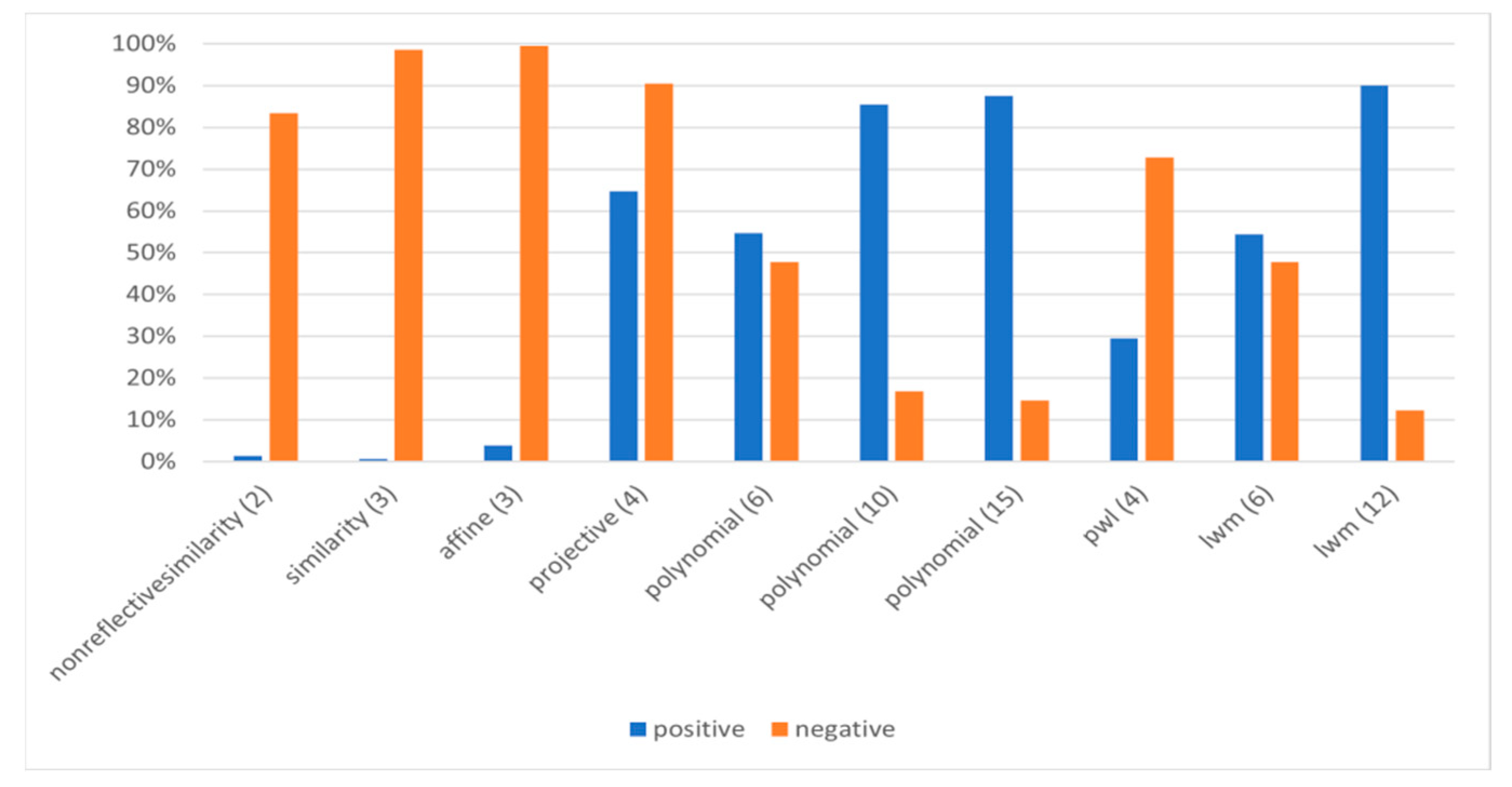
Each of the available transformation models was tested on a pair of stereoscopic images obtained during bench tests (“test position”). After the initial processing of the images, to extract the markers from the images, the stereo correspondence between the markers found by the tested algorithm was compared with the known stereo correspondence of the measurement images. For each transformation model, the influence of the scope of searching the vicinity of a given marker on the correctness of matching markers (finding stereo correspondences between a grid of markers recorded on a pair of measurement images) was checked, as well as the effect of removing markers from images after prior classification. The search range was either small, medium, or large, which corresponded to 5, 10, or 50 px (pixels), respectively. The results of this are presented in Figure 3.

Measurement images show the same scene imaged from two different positions. This makes each corresponding object (marker grid) in the images significantly different from the other [11,20,21,22]. Depending on where the pick holder was mounted on the side surface of the cutting head, the imaged pattern can be deformed to a different extent. In addition, although we are dealing with a perspective transformation, we can see that the transformation models based on ten or more pairs of matching points ensured the correctness of matching markers at a level of at least 85%. However, due to the difficulty of detecting and matching mutually corresponding points in the images of the stereo couple, a geometric transformation model was adopted based on ten pairs of points, i.e., a third-degree polynomial transformation [23]:

$$\left\{\begin{array}{l}X=t_X+ax+by+c{x}^2+dxy+e{y}^2+f{x}^3+g{x}^{2}y+hx{y}^2+i{y}^3\\ Y=t_Y+jx+ky+l{x}^2+mxy+n{y}^2+o{x}^3+p{x}^{2}y+qx{y}^2+r{y}^3\end{array}\right.$$

(2)

or, in matrix notation:

$$\mathrm{P}=\mathrm{t}+\mathrm{Ap},$$

(3)

where:

X, Y are coordinates of the point in the image coordinate system after transformation,

x, y are coordinates of the point in the coordinate system of the original image,

t_X, t_Y are the translation of a given axis of the coordinate system,

a ÷ r are coefficients determined based on the coordinates of the fit points,

P is the leading vector of the point in the image coordinate system after transformation,

p is the leading vector of the point in the coordinate system of the original image,

t is translation vector,

A is a transformation matrix.

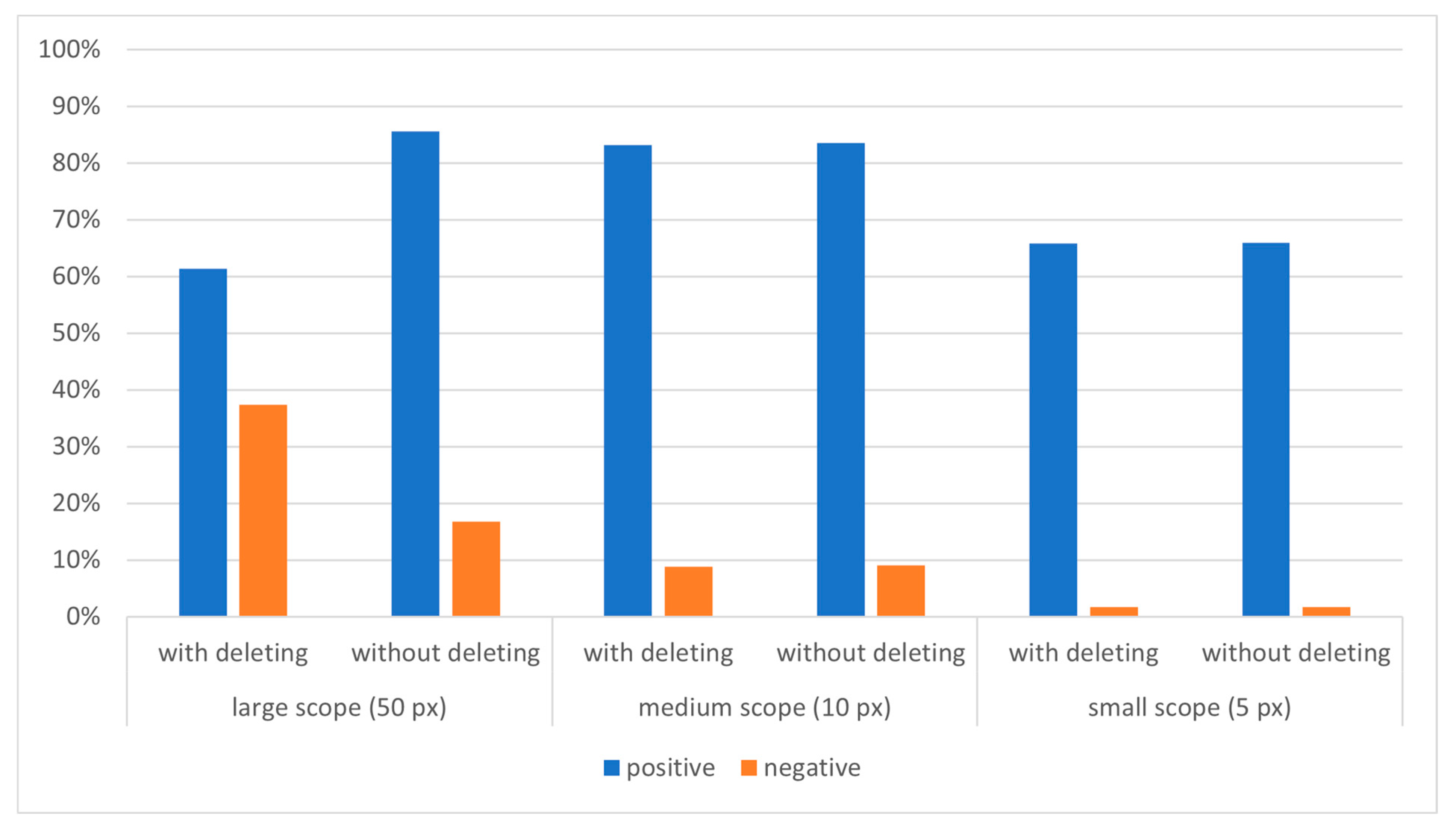
The results for this type of transformation are shown in Figure 4. It can be seen that the small search range (5 px) significantly reduced the number of incorrectly classified markers. Unfortunately, however, it also had a negative impact on the number of correct indications. A large search range (50 px) when removing previously classified markers ensured correctly matched markers at a level of 62%, with incorrectly matched markers at 38%. The number of correct indications when not removing previously classified markers was 86% and those incorrect were found to be 17%. Since the classified markers were not removed from the images, there occurred a situation where one marker could be matched several times. The medium search range (10 px) guaranteed a match of almost 85%, and a negative match of 8%, regardless of whether or not the previously classified markers were removed from the images. The remaining 7% of the marker grid points were not matched. Similarly, regardless of whether or not the previously classified markers were removed from the images, the number of correct indications for the small search range (5 px) was 67%, and incorrect was 1%. In general, to reduce the risk of incorrectly matching of a pair of markers in the images, it is advised that the smallest possible search range (≤10 px) is used. In doing so, the share of incorrectly classified points should not exceed 10%.

3. The Use of a Genetic Algorithm in the Process of Matching Points Selection

Adjusting (or transforming) the images based on the adopted polynomial model required entering the coordinates of ten points that are common in both images. These were the so-called ‘matching points’. During processing, these points were selected from a set of mesh points projected by laser onto the cutting head’s side surface. Preliminary experiments with the selection of matching points from among 2601 points displayed by the laser showed that their location had a significant impact on the quality of image alignment, and on the correct identification of corresponding points in the image from the left and right cameras. Considering the number of matching points required, there were 3.83 × 10²⁷ possible combinations. Therefore, the best way to solve this problem was to perform optimization for the adopted objective function [24]. However, due to the nature of the optimization task (the discrete form of the arguments of the objective function, i.e., the numbers of points of the grid projected by the laser), the use of classical optimization methods (e.g., gradient methods or non-gradient searches for the extreme function) would be of little use. For this reason, an evolutionary algorithm was used [25,26]. Such algorithms are stochastic iterative algorithms in which the search for the coded space of potential solutions is carried out in a targeted manner. In the subsequent steps, certain elements of the approximate solutions found so far were used to obtain the optimal solution. An important property of this type of algorithm is its ability to avoid becoming stuck in local extremes. Hence, they are often used in optimization tasks and the modeling of phenomena in many fields of science and technology [27,28,29,30,31].

The optimization task consisted of finding a set of 10 matching points that would, after polynomial transformation of the images, provide the maximum number of correctly matched markers. Since the use of the genetic algorithm requires experience and a relatively large number of iterations, many tests were carried out to estimate the parameters of the genetic algorithm, including the number of individuals, number of generations, probability of mutation, and crossing [32,33,34,35].

An application was subsequently developed using the conventional operators of selection (roulette method), crossing (single point with random split point), and single point mutation. Binary chromosome coding was used in both images, with each of the ten chromosome genes indirectly containing information about the coordinates of the selected marker (Figure 5a). Since 2601 points had to be encoded, 12 bits were needed, and the initial population was drawn each time. Next, after assessing the adaptation of the resulting population (Figure 5b), another generation was created based on selection by the roulette method (Figure 5c,d). The probability of selecting a given chromosome is given by:

$$p_s\left(c{h}_i\right)=\frac{F\left(c{h}_i\right)}{{{\displaystyle \sum }}_{i=1}^{n}F\left(c{h}_i\right)}$$

(4)

where:

p_S is the probability of selecting a chromosome,

ch is chromosome,

F is fitness value,

n is population size.

The applied one-point mutation method changed the value of the entire gene, and not just a single allele. Initially, the mutation probability was 0.03, and the crossover probability was 0.6 (Figure 5e). The nature of the problem of mapping the surface of the cutting-head machine when positioning the pick holders makes it particularly important to correctly identify the markers displayed there. These were located directly in the vicinity of the pick holder base (which has dimensions 40 × 20 mm), in an area with a radius of approximately 30 mm from the center of the projected pattern. Therefore, during the experiments, the correctness of fit in this area was checked for the obtained results. As well as the influence of the number of individuals and the number of generations, the influence of the size of the area around the center of the marker grid was investigated, and its fitness function was assessed. This area was a circle with its center in the direct middle of the grid of points projected onto the side surface of the cutting head, and comparative radii were r = 15 mm, r = 22.5 mm, r = 30 mm, r = 37.5 mm, and r = 45 mm. This influenced the size of the population of points taken into account for the assessment of the adaptation function (N_POP), given by:

$$G=\frac{N_{POZ}}{N_{POP}}\to 1,\mathrm{wherein}$$

(5)

$$N_{POZ}\le N_{POP}$$

(6)

where:

G is fitness value,

N_POZ is the number of positively matched markers,

N_POP is the size of the population of points taken into account for the assessment of the fitness function.

The correctness of the fit was assessed for all markers, as well as those located within the radius R = 30 mm from the center of the standard. To select the appropriate number of individuals and the number of generations, many simulations were carried out.

Figure 5. The next steps in the operation of the simple genetic algorithm: (a) selection of the initial population; (b) assessment of population adaptation; (c) selection by roulette method; (d) crossing with a randomly selected split point (locus); (e) mutation of a randomly selected gene.

Figure 5. The next steps in the operation of the simple genetic algorithm: (a) selection of the initial population; (b) assessment of population adaptation; (c) selection by roulette method; (d) crossing with a randomly selected split point (locus); (e) mutation of a randomly selected gene.

It was found that the larger the population of individuals, the greater the number of correctly classified points, especially in the central area of the point grid (Figure 6). When considring number of individuals, the population consisting of 400 individuals gave the best adaptation. The number of correctly classified markers here was close to 77% for the entire pattern, and 79% for the area with radius r = 30 mm. Genetic algorithms generally converge quickly to the optimal solution, however, a large number of generations is not indicated due to the need for long computational times [36]. Therefore, the conducted simulations examined the evolution of the population for 20 generations. 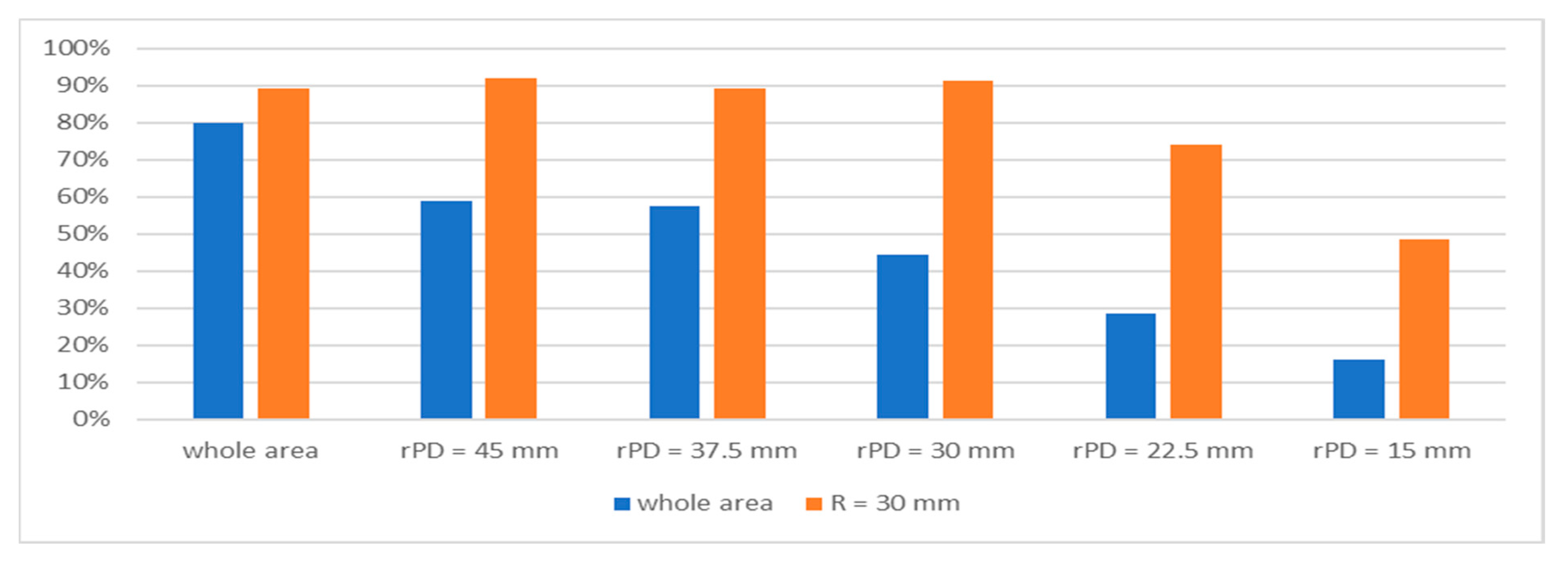In most of the simulations, the genetic algorithm converged after only a few generations, and the result was not improved with further iterations (Figure 7). The size of the area in which the adaptation function was checked (the number of points around the center of the grid) had a large impact on the results (Figure 8). Assessing the fit function over the entire area guaranteed a fit of at least 91% for the complete marker grid, and 76% for the area with radius R = 30 mm. On the other hand, the assessment of the adaptation function in the area with radius R = 30 mm guaranteed an adjustment of 89%, with 80% for the entire marker grid. Since it is particularly important to fit the central area of the marker grid, a further study was conducted with the objective function of assessing the matching of markers in the area within the radius R = 30 mm at the center of the pattern. Evaluation of the algorithm’s adaptation function in smaller areas only degraded the effectiveness of the alignment.

The probability of crossing did not significantly affect the correctness of matching the image markers from the left and right cameras, or the rate of convergence by the genetic algorithm (Figure 9), especially in the central area of the mesh (limited circle with radius R = 30 mm). In the studied range, the probability of crossing the proportion of correctly matched points varied between 87 and 92% for the entire network of markers, and between 59 and 84% for the central area. On the other hand, the increase in the mutation probability improved the quality of the fit for the entire area of the grid of points (Figure 10). It also had a positive effect on the fit in the central area of the mesh. However, it also increased the number of generations needed to achieve the best fit. Additionally, it prevented the algorithm from becoming stuck in a local minimum. In subsequent experiments, two sets of matching points were obtained for the values of the mutation operator p_M 0.03 and 0.09, and the crossing operator, which was equal to p_C 0.6. These variants are marked accordingly as W1 and W2, respectively.

By way of example, Figure 11 shows the arrangement of the fitted points (a,b) for the mutation rate p_M = 0.03. The quality of image matching was presented in the form of an anaglyph (c), and a set of correctly classified points (d). As can be seen in Figure 11, the classification of the points in the central part of the images and at their lower right corner was correct. Only 20% of all markers were incorrectly classified. However, this mainly applied to points on the periphery of the images. Designated sets of 10 matching points were tested on three pairs of measuring slips, and the images represent various deformations of the marker grid projected onto the side surface of the cutting head during the positioning of the pick holder.

4. Determination of the Effectiveness of Finding Stereo Correspondence of Raster Images with the Use of the Developed Method

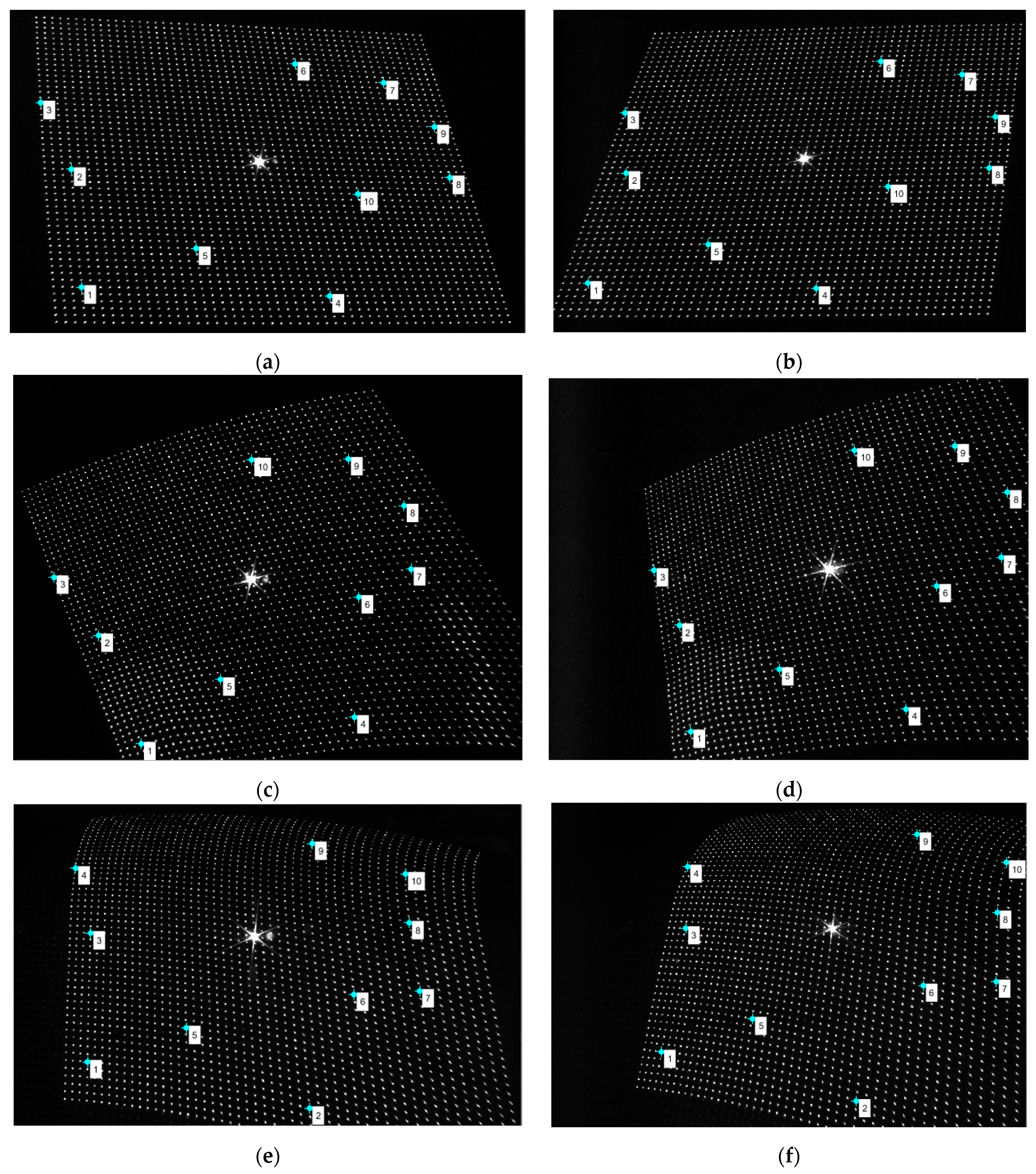
The deformation of the marker grid with three pairs of measuring points resulted from the shape of the surface onto which the grid of measuring points was projected, as well as the camera settings. The images sequentially show the grid of measurement points, which was either slightly deformed, moderately deformed, or strongly deformed (Figure 12). The data on the stereo correspondence of the marker grid for the prepared images was acquired and compared with the stereo correspondence results obtained with the developed method. For the transformation of the test images, two sets of 10 matching points characterized by the best adaptation were used (variants W1 and W2). The pattern of markers in the images for the test position was rotated by 45° to obtain the pattern recorded in the images prepared for testing. Therefore, the tests were performed twice for two different orientations of fit points to marker pattern rotated by 180°, to assess how the rotation of these points on the images affected the final result. The presented results show the number of correctly matched markers in the entire pattern and at its center. Depending on the deformation of the pattern in the pairs of images, the number of correctly matched markers for the entire mesh area ranged between 62 and 100%. Meanwhile, the number of correctly classified markers in the area with radius R = 30 mm ranged from 94 to 100%. The first of the selected sets of points (W1) was characterized by a better fit of the marker grid for all the sample pairs of measurement images, especially in the central area (r ≤ 30 mm). Therefore, further results are presented for this set of 10 matching points (Figure 13). The results also showed that rotating the matching point set clockwise increased the number of correctly recognized markers for both selected fit point sets (Figure 14).

For the measurement of the distance between the pick holder base and the side surface of the cutting head, it was important to minimize the number of incorrectly matched markers, even at the expense of the number of correctly matched markers. This is especially true of the central image area, which was located directly under the base of the pick holder. For the sake of formalities, the impact on the quality of matching the marker grid in three selected pairs of measurement images for three different search ranges was examined, both with and without removing previously classified markers from the images (Figure 15). For each case, along with an increase in the degree of deformation of the marker grid, the effectiveness of matching the marker grid decreased. Removing classified points from images with a large search range (50 px) significantly reduced the number of correctly matched markers and increased the number of incorrectly matched markers (Figure 16a). Depending on the level of deformation of the marker grid on pairs of images, this effect appeared with different intensities. Markers remaining on the images with a large search range (50 px) significantly reduced the number of incorrect indications in favor of correct ones (Figure 16b). In medium search ranges (10 px), whether or not the previously classified points were removed from the images did not significantly affect the results (Figure 16c,d). This is because the effectiveness of matching markers decreased as the scope of the search was reduced (the number of correctly and incorrectly classified points decreased). In contrast, in the case of a small search range (5 px), the matching results influenced by whether or not previously classified markers had been removed (Figure 16e,f). Here, as in the previous cases, the quality of the adjustment depended on the level of deformation of the marker grid in the images. The use of this small search range for markers in the images was characterized not only by the smallest number of incorrectly classified marker pairs, but also by the smallest number of correctly classified markers.

Since we aimed to maximize correct results and minimize incorrect results, it was more appropriate to choose a small search range (5 px) without removing classified points (Figure 16f), or a medium search range (10 px) with points removed (Figure 16e). The effects of the latter procedure are shown in Figure 17. Depending on the degree of deformation of the marker grid, the number of correctly matched markers was in the range 69–100% for the variant W1 rotated to the left, and the number of incorrectly matched points did not exceed 22%. For the right-turned W1 variant, the number of correctly matched marker pairs was in the range 82–98%, and incorrect was below 14%. For the W2 variant, the number of correctly matched markers, depending on the degree of distortion of the marker grid and the pattern rotation, was in the range 62–98% and incorrect was below 28%.

5. Proposal for the Technical Implementation of the Elaboration of Finding Stereo Correspondence of Measurement Images

The proposed method of matching raster images requires in the first stage the indication of a set of 10 matching points, which are selected based on research. For the algorithm that searches for them and classifies them into pairs (and to recognize these specific markers from the rest), they should be distinguished in some way, preferably by shape or size. It is also possible to display separately the pattern of a set of ten markers and the pattern of the measurement markers. The laser works by diffracting one light source (2601 points). During the acquisition of measurement images, the laser was mounted on the gripper that positions a given pick holder to the side surface of the cutting head. Because the settings of each pick holder differed depending on the values describing the position in space of the pick tip, the size of the displayed pattern on the side surface changed. Depending on the shape of the side surface in the place where the pick holder was mounted, the pattern of markers displayed on it was characterized by different deformations. In the application of the laser, it is impossible to set up ten lasers in such a way that their beams intersect together at one point using beams generated by diffraction grating. Therefore, the use of a set of 10 lasers projected parallel to each other was considered. Using this method, the images from the stereovision system cover approximately the area of 100 × 100 mm, and the grid size of the markers displayed on the side surface of the cutting head ranges from 94 × 94 mm to 98 × 98 mm. The use of a laser constructed in this way ensures that the set of matching points will always be visible on the measurement images, regardless of the deformation of the marker grid. The marker grid displayed from one point is subject to deformation caused by, among other factors, the different lengths of rays falling onto the side surface (Figure 18). Therefore, we decided to investigate the effect of the clustering of the matching points towards the marker pattern’s centre on the effectiveness of matching the marker grid between the measurement images. For this purpose, a series of simulations were performed in which the area around the center of the marker pattern in the images was gradually reduced, from which the genetic algorithm selected the matching points for the image transformation. The entire area of the grid was used with r_PD = 15 mm, r_PD = 22.5 mm, r_PD = 30 mm, r_PD = 37.5 mm, and r_PD = 45 mm.

The results showed that with the reduction of the area around the center of the marker pattern in the images (from which the genetic algorithm selected the matching points for the image transformation), the optimal area for best matching of the marker pattern recorded on the pair of images decreased (Figure 19). The best fit for the entire pattern was obtained when a set of points matched among all pattern markers were used for image transformation. In the case when a set of matching points was used for image transformation among markers located in the radius r_PD = 30 mm around the center of the pattern, the best fit was obtained for the area with radius R = 30 mm (however, with lower effectiveness of fitting points over the entire grid).

6. Method of Finding the Stereo Correspondence of Matching Points

The condition for finding the correct stereo correspondence of the markers recorded on images, using the method proposed in this paper, is to find with 100% efficiency the stereo correspondence between the matching points distinguished in the pair of images [37]. Incorrect fittings at this stage will deform the image and, as a result, lead to incorrect or missing matches. It should be noted that if all fitted points are not matched, the image cannot be transformed. To find the stereo correspondence of the matching points, the classical approach (searching for points on a pair of images with epipolar lines) can be used [38]. The same point has the same y-coordinate in both images, and if there are more such points on the images, they successively count towards increasing values of the x coordinates in the image.

For all 14 pairs of images considered in this study, finding the matching points with this method gave 100% effectiveness.

7. Summary and Conclusions

The use of a stereovision system on a robotic assembly station to measure the distance between the bases of pick holders and the side surface of the mining machine’s working unit is justified by metrological requirements. An important step in measurement with the use of the stereovision system is to find the stereo correspondence of points in the images from the left and right cameras.

The presented results show that the developed method of matching raster images allows stereo correspondence to be found automatically for the grid points of markers recorded on a pair of images. Since the use of commonly known techniques for finding stereo correspondence between images did not give satisfactory results, a different approach was proposed. This approach consisted of transforming the right image into the left image using a polynomial model, and subsequently finding stereo correspondence between the points of the marker grid recorded on both images.

During numerical and experimental research:

• The image transformation model was determined to ensure the best fit of the marker grid on pairs of images and thus the number of matching points necessary to carry it out.
• Using optimization methods, the distribution of matching points was determined to ensure the best fit between images.
• It was found that the developed method was characterized by different yet satisfactory effectiveness, depending on the deformation of the marker grid.
• The most important task from a metrological point of view is the possibility of minimizing the number of incorrectly matched points, and maximizing correctly matched points, within the area at the central part of the marker grid, i.e., directly under the base of the pick holder.
• To develop a laser enabling the implementation of the presented measurement task, the proposed method examined the effect of concentration around the center of the grid on the effectiveness of matching markers.

Based on the results of the research, the following conclusions were drawn:

(a)

Non-linear image transformation models based on ten or more pairs of matching points for image test positions ensures at least 85% correctness of matching markers

(b)

To reduce the risk of incorrect matching of markers in the images, it is advised to use the smallest possible search range (≤10 px) with the removal of points.

(c)

The parameterization of the adopted model using geometric transformation of images to match measurement points, regardless of the orientation of the marker grid, ensures high efficiency of finding corresponding markers in images recorded by the right and left cameras of the stereovision system. Depending on the degree of deformation of the registered marker grid (resulting from the shape of the surface on which they were displayed), the proportion of correctly fitted measurement points was as follows:

• For a small deformed marker grid: 98 to nearly 100% correctly fitted markers, with almost 100% correctly fitted markers in the central area of the marker grid (limited circle with radius R = 30 mm);
• for a medium deformed grid of markers: 80–89% correct matches, while in the central area of the marker grid the share of these points ranged from 93 to 100%;
• for a large deformed marker grid: 53 to 82% correct matches, in the central area of the marker grid the share of correctly fitted markers in the right and left image ranged from 82 to 100%.

Due to technical limitations (making it impossible to distinguish selected matching points from the marker pattern), a projection device was equipped with 10 lasers displaying the matching points on the side surface of the working part of the cutting machine. This allowed us to maximize the effectiveness of the marker alignment within the area of the images where the set of matching points was visible.

The proposed method of matching can be successfully used to reconstruct a scene using active stereo vision, and provides an important step in the analysis of measurement images in multi-image systems. It has been developed for measuring systems within adaptively controlled robotic assembly stations of working units in mining machines, such as roadheaders, longwall shearers, asphalt milling machines, crushers, or river dredgers. However, it can also be used wherever necessary to assess the correct course of a technological process, based on the measurement of certain geometric quantities. Measurements performed with visualised techniques can be carried out online in real-time, ensuring fast and reliable processing. This is of particular importance in robotic technologies, where it is possible to correct the process parameters during implementation based on measurement results.