A Period-Based Neural Network Algorithm for Predicting Building Energy Consumption of District Heating

Abstract

Northern China is vigorously promoting cogeneration and clean heating technologies. The accurate prediction of building energy consumption is the basis for heating regulation. In this paper, the daily, weekly, and annual periods of building energy consumption are determined by Fourier transformation. Accordingly, a period-based neural network (PBNN) is proposed to predict building energy consumption. The main innovation of PBNN is the introduction of a new data structure, which is a time-discontinuous sliding window. The sliding window consists of the past 24 h, 24 h for the same period last week, and 24 h for the same period the previous year. When predicting the building energy consumption for the next 1 h, 12 h, and 24 h, the prediction errors of the PBNN are 2.30%, 3.47%, and 3.66% lower than those of the traditional sliding window PBNN (TSW-PBNN), respectively. The training time of PBNN is approximately half that of TSW-PBNN. The time-discontinuous sliding window reduces the energy consumption prediction error and neural network model training time.

1. Introduction

The construction industry produces significant carbon dioxide emissions and leads to considerable energy consumption in modern society [1,2,3]. In China, heating in northern cities consumes 20% of the total energy consumption of buildings [4,5]. Since the mid-1990s, China has begun to develop central heating with power plants as heat sources. The heating mode is mainly based on cogeneration supplemented by new energy sources, such as ground source heat pumps. The fuel for cogeneration is coal, and haze has become a severe environmental problem [6,7]. With China’s emphasis on environmental protection, urban district heating (DH) has become mainstream. However, the operation management and control technology of heating systems are still relatively simple. Overall, intelligent heating cannot keep up with the development of the scale of heating required.

DH is an essential public energy service consisting of heat sources, heat supply networks, and heat consumers. Due to the lack of accurate DH loads, energy system operating strategies often operate inefficiently [8,9]. This results in a vast and unnecessary waste of energy. Excessive and uneven heating is currently China’s largest source of heat loss. Because the heating system has the characteristics of a large heating scale, strong coupling, high thermal inertia, and challenging-to-determine thermal parameters, there is always a time lag between the balance of supply and demand [10,11,12].

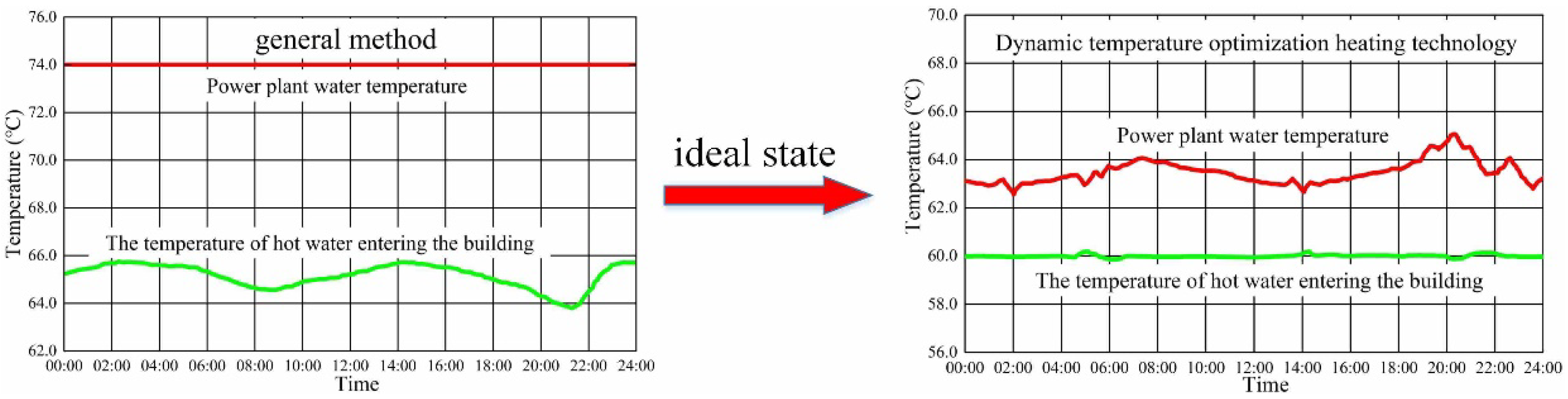
The traditional control method of DH is to keep the outlet water temperature of the power plant unchanged. The temperature of the water entering the building fluctuates, as shown in Figure 1. However, under ideal conditions, the indoor temperature of the building remains constant, at 20 °C or 18 °C, for example [13]. As a result, the outlet water temperature of the power plant fluctuates. Accurate heat load prediction can reduce this imbalance between heating supply and demand, thereby reducing the energy consumption of DH.

To achieve the above ideal state, building energy consumption prediction is needed. Currently, there are two main methods for producing energy prediction: physics models and data-driven models [14,15]. The physics model, also known as the white-box model, refers to the modeling of building energy consumption based on the heat transfer mechanism. The relevant heat transfer equations are then solved to obtain building energy consumption predictions. Commercial software such as EnergyPlus [16], Transient System Simulation Tool (TRNSYS) [17,18], and Designer’s Simulation Toolkit (DeST) [19,20] utilize physics models to predict building thermal loads. However, these models often require a large number of building characteristic parameters. Some parameters are not readily available. Additionally, some parameters will change over time, so we can only estimate these parameters and cannot obtain accurate values. At the same time, the calculation time is prolonged. Due to the inability to obtain accurate parameters, complex physics models often cannot achieve the expected prediction accuracy. Although some of the above shortcomings can be avoided if simple physics models are applied, their prediction accuracy often struggles to meet application requirements.

With the development of big data technology and machine learning (including deep learning), these technologies are gradually being introduced into building energy consumption prediction, resulting in data-driven models [21,22,23]. The data-driven model refers to the energy consumption prediction model formed by mining historical heating data, training, and fitting. It predicts heating energy consumption based on heating data as the core basis. This energy consumption prediction model does not need to know the physical relationship between the heating data, which simplifies the model [24]. Data-driven models require considerable data and computational effort. Without a powerful GPU, some data-driven models may take tens of hours to complete model training. However, these shortcomings are no longer significant with recent advances in instrumentation and computing power. Standard data-driven models include linear models [25], decision trees [26,27], support vector machines (SVMs) [28,29], gradient-boosted trees [30,31], and deep learning models [32,33,34].

We propose a periodic-based neural network (PBNN) to predict building energy consumption. The main innovation of this work is the application of a new data structure based on the periodicities of building energy consumption. According to the period of energy consumption data, a time-discontinuous sliding window is proposed. Periodic features are triangularly transformed. After data preprocessing, the training data enter the CNN-LSTM model. The convolution kernel scale of the convolutional neural network (CNN) is set to 12 according to the period of energy consumption data. Long Short-Term Memory (LSTM), traditional sliding window PBNN (TSW-PBNN), and PBNN are compared to demonstrate the effectiveness of the data structure introduced in this paper.

The main contributions of this paper are summarized as follows:

1.

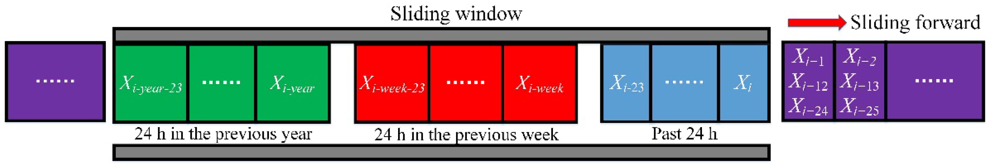
A data structure suitable for building energy consumption prediction is proposed. Sliding windows consist of temporally discontinuous data. The sliding window consists of building data for the past 24 h, 24 h in the previous week, and 24 h in the previous year.

2.

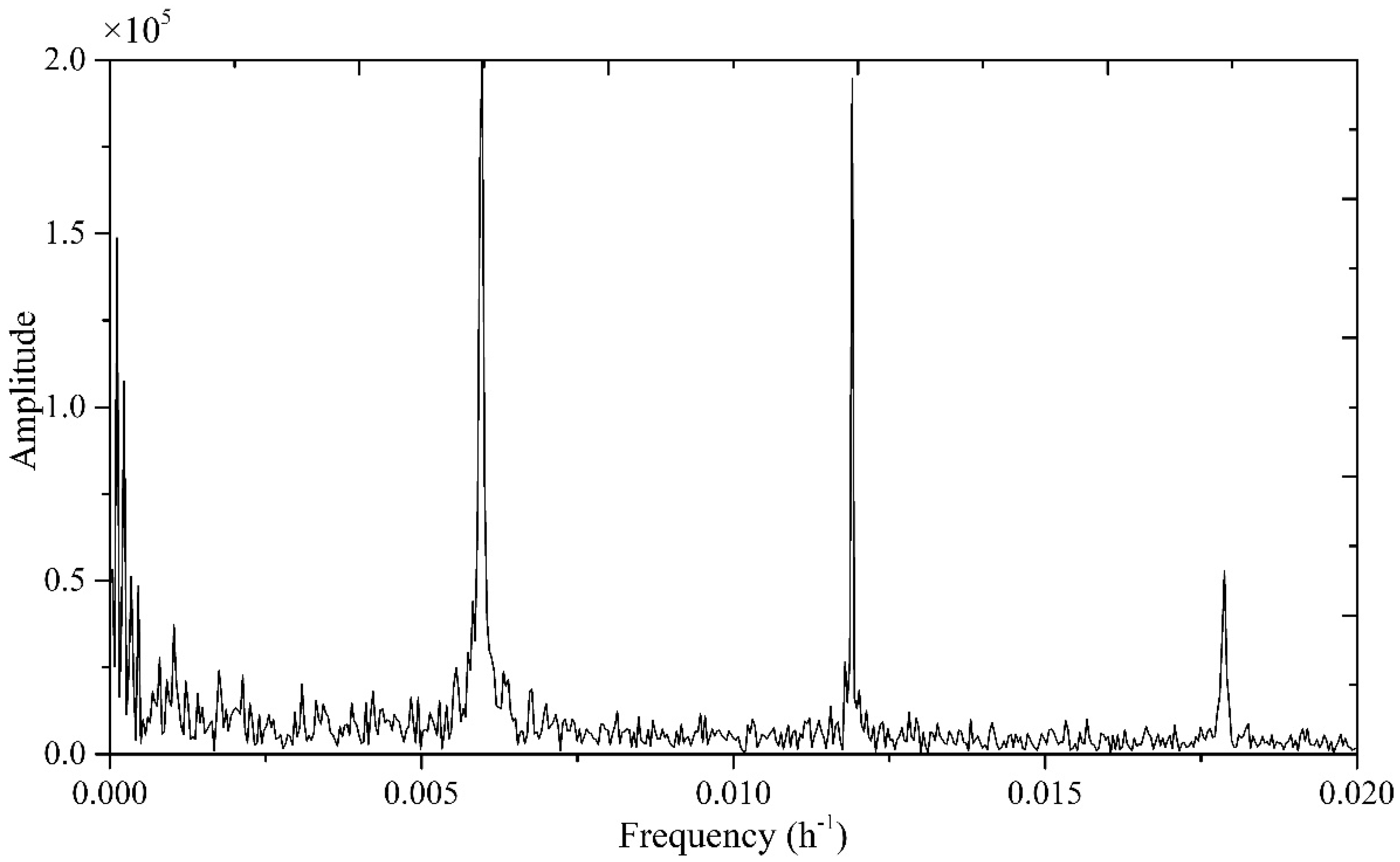
It is demonstrated through Fourier transformation that there are daily, weekly, and annual periods in building energy consumption. The CNN convolution kernel size is set by the period of the energy consumption data.

3.

The time-discontinuous sliding window drastically reduces the model training time and energy consumption prediction error. The particular sliding window structure allows a sample to contain more information through a specific sliding window structure.

4.

When the distribution of building energy consumption in a month is closer to the distribution of building energy consumption in the whole year, that month’s energy consumption prediction error is lower.

The structure of this paper is as follows. Section 2 describes the data sources and discusses the period of energy consumption data through Fourier transformation. The traditional sliding window and time-discontinuous sliding window are elaborated. Section 3 reports on the baseline model, LSTM, PBNN, and TSW-PBNN. Section 4 compares the prediction performance of LSTM, TSW-PBNN, and PBNN for building energy consumption. The conclusion is presented in Section 5.

2. Materials and Methods

2.1. Data Sources

The data for this paper come from the Great Energy Predictor III (GEPIII) machine learning competition [35]. Over 20 million training data points from 2380 energy meters were collected for 1448 buildings from 16 sources [36]. The data include three years of hourly time series data for each meter and weather information. There are leaked data in the competition [37], including hourly measurement data from 1 January 2016 to 31 December 2018. This competition aimed to find the best model for predicting the energy consumption of all buildings. The main models used in the competition were Light Gradient Boosting Machine (LightGBM), CatBoost, XGBoost, and Multi-Layer Perceptron (MLP).

We focus on the single energy meter prediction problem in this work. The impact of the time series on the forecast results is fully considered. By reorganizing the competition data, the features and targets are shown in

Table 1. Data description in GEPIII.

Property	Name	Implication
time	timestamp	When the measurement was taken
feature	air temperature	Degrees Celsius
feature	cloud coverage	Portion of the sky covered in clouds, in oktas
feature	dew temperature	Degrees Celsius
feature	precip depth 1 h	Precipitation in millimeters over 1 h
feature	sea level pressure	Millibar/hectopascals
feature	wind direction	Compass direction (0–360)
feature	wind speed	Meters per second
feature	hour	The hour (0–23) corresponding to the timestamp
feature	weekday	The weekday (0–6) corresponding to the timestamp
feature	week of year	The week of year (1–53) corresponding to the timestamp
feature	year	2016, 2017, or 2018
target	meter reading	Energy consumption in kWh (or equivalent); real data with measurement errors

.

The sample data are combined, as shown in Figure 2. T1, the timestamp, is a time index, and this parameter is not directly used in the prediction model. Feature X consists of weather data, date–time data, and historical sensor data. Weather data consist of air temperature, cloud coverage, dew temperature, precipitation depth at 1 h, sea level pressure, wind direction, and wind speed. Date–time consists of the hour, weekday, week of the year, and year. Historical sensor data are the energy meter readings. Feature X contains the above data for multiple past moments simultaneously. The model-predicted value Y is the T1-predicted target value, which refers to the energy meter measurement in the next 1 h, 12 h, and 24 h. The energy prediction model in this paper is a multi-objective prediction problem.

There are two main approaches to long-term prediction for time series problems [38,39]. One of them is to use the rolling prediction method, which assumes that the minimum granularity of time is hours. According to the historical data at time t, the model is trained to predict the building energy consumption at time (t + 1) (with hour as the unit). Once the building energy consumption at time (t + 1) is obtained, it is used as input data to predict the building energy consumption at time (t + 2). By analogy, the energy consumption of the building at the subsequent time is obtained. Such iterations will continue until the time (t + 24). The building energy consumption at times (t + 1), (t + 12), and (t + 24) is selected from the calculation results, which is the model prediction result. Another method is the non-rolling prediction method, which fixes the time interval between the prediction target and the input. The input is historical data at time t, and the output is a vector of building energy consumption at times (t + 1), (t + 12), and (t + 24). The model is directly trained end-to-end. The advantage of the rolling forecast method is that the model is simple, and it is convenient to predict the building energy consumption after any full hour. Its disadvantage is that the prediction error generally increases over time. The non-rolling forecast method minimizes the weaknesses of the rolling prediction method. We applied the non-rolling forecast method to predict the energy consumption of buildings.

2.2. Periodicity of Energy Consumption Data

Time series data of building energy consumption are often periodic, which is an important feature that distinguishes them from general time-series data. The building operation law is affected by both social processes and the Earth’s natural cycle. The periodicity of energy consumption in each building may not be the same. For example, a college building has a cycle of semesters and vacations. However, general buildings usually have the following three periodicities: daily persistence, weekly persistence, and weekly one-year-ago persistence. For example, 2 July 2018 is the Monday of the 27th week of 2018. According to the previous three periodicities, 10:00 on 2 July 2018 corresponds to 10:00 on 1 July 2018, 10:00 on 25 June 2018, and 10:00 on 3 July 2017. The latter date, 3 July 2017, is the Monday of the 27th week of 2017. There is a close relationship between the building energy consumption at 10:00 on 2 July 2018 and the building energy consumption on the corresponding date, which is shown in Figure 3.

Next, we verify the above conclusions with GEPIII data. The building with ID185 in the GEPIII competition dataset is selected as the research object. The primary use of the building is education. The building area is 84,300 square feet. Three-year energy consumption data of Building 185 were leaked, so the complete hourly energy consumption data, from 1 January 2016 to 31 December 2018, can be found on the Internet [37]. Figure 4 is a graph of the time–energy consumption data for Building 185. The daily energy consumption is replaced by the energy consumption at 0 o’clock. The abscissa is directly represented by the time series, where 0 means 1 January 2016 and 1 means 2 January 2016. The ordinate is the building energy consumption. The three-year hourly data of Building 185 contain a total of 26,294 samples.

The periodicity of building energy consumption is not readily available, as shown in Figure 4. For this purpose, a Fourier transformation was performed on 26,294 points of hourly energy consumption data [40]. A frequency–amplitude diagram was obtained, as shown in Figure 5. The unit of frequency is 1/hour (h⁻¹). The frequencies corresponding to the seven largest amplitude peaks are 0.0001141 h⁻¹, 0.0357 h⁻¹, 0.00594 h⁻¹, 0.0416 h⁻¹, 0.0119 h⁻¹, 0.00598 h⁻¹, and 0.0427 h⁻¹. They are converted into periods of 8764 h, 28 h, 168 h, 24 h, 84 h, 167 h, and 23 h. These seven periods can be divided into four groups, namely, [23 h, 24 h, 28 h], [84 h], [167 h, 168 h], and [8764 h]. The first group corresponds to the daily period. The second group corresponds to the half-week (3.5 days) period. The third group corresponds to the weekly period. Moreover, the fourth group corresponds to the annual period. The year 2016 consisted of 366 days, so 8764 h is slightly more than 8760 h (365 days). The analysis results of Building 185 support the conclusion that there are several periodicities in building energy consumption. The analysis results suggest 12-h periodicity in building energy consumption.

2.3. Traditional Sliding Window and Time-Discontinuous Sliding Window

The theoretical calculation of the heating system is often carried out based on the ideal working conditions in a steady state. Actual operating conditions must be analyzed using dynamic methods. Because the energy consumption of buildings is affected by factors such as thermal inertia, outdoor temperature, and solar radiation, there are significant errors in the energy consumption prediction based on a data sample from a single moment.

A sliding window containing data samples of a specific time range could better describe the building energy consumption problem. By introducing the sliding window, the noise of the original data can be reduced, and the prediction results will be more stable. At the same time, this can reduce the impact of outliers and error values on the prediction model [41].

The sliding window includes the sample itself and the specified number of samples preceding it, which increases the prediction accuracy of the energy consumption model. The sliding window can be defined as $X_i^j$, as shown in Equation (1).

$$X_i^j=\left(x_{i-j},\cdots ,x_{i-1},x_i\right)$$

(1)

where j is the window size and i is the timestamp of the model prediction. x_i is a data sample at one moment.

The model’s predicted value is $Y_i^3$, as shown in Equation (2).

$$Y_i^3=\left(x_{i+1},x_{i+12},x_{i+24}\right)$$

(2)

To be precise, the energy meter measurements in x_i+1, x_i+12, and x_i+24 are the model’s predicted values. The sliding window is shown in Figure 6, referred to as a traditional sliding window (TSW) because the data samples within the sliding window are continuous in time. When the sliding window keeps sliding forward, the energy consumption prediction model constantly makes predictions.

Since building energy consumption has periodicities of days, weeks, and years, we fill the sliding window with the data of the corresponding date. The time-discontinuous sliding window is shown in Figure 7. The sliding window size is still 72 h. The sliding window consists of the related data of the past 24 h, 24 h of the past week, and 24 h of the previous year (considering the weekly characteristics). Time is no longer continuous within the sliding window. From the perspective of energy consumption prediction, the sliding window composed in this way contains more information. Compared with the building data of the past 72 h, the sliding window shown in Figure 7 reduces the energy consumption prediction error. The following calculation results prove the above conclusion. The main innovation of this paper is the introduction of time-discontinuous sliding windows into neural network algorithms.

3. Modeling and Methodology

This section introduces data preprocessing, hyperparameter optimization, evaluation criteria, and the four models used to predict building energy consumption.

3.1. Data Preprocessing

Data preprocessing is critical for neural network model training. The neural network algorithm is an end-to-end algorithm, and the intermediate process does not need to be manually designed. However, if the unprocessed data are directly entered into the neural network model, this can cause problems such as long model training time and significant error in the model prediction results. In severe cases, it may even cause model training failure. In this paper, the data are mainly preprocessed by outlier removal, missing value filling, the periodic processing of some features, and min–max normalization. Outlier removal is primarily used to detect datasets and remove unreasonable energy consumption data and weather parameters. Due to occasional instrument failures, data are missing for some moments in the dataset. Missing data values are filled with the average data value for that day.

The characteristics of wind direction, hour, weekday, and week of the year are periodic and discrete. In the general literature, one-hot encoding is performed for such features. However, if these features are one-hot encoded in this paper, there will be too many features, and other features’ information will be masked. Here, trigonometric functions are introduced to deal with such features, and the calculation formula is as follows:

$$x_{new}=\left(\sin \left(\frac{2\pi }{T}x\right)+1\right)/2$$

(3)

where x_new is the feature obtained after triangular transformation, x is the original feature, and T is the period of the feature. Through Equation (3), the converted features can better reflect the periodicity and take values between [0, 1].

Finally, min–max normalization is introduced to convert the scale of all variables to the range of 0–1. This data normalization technique consists of performing a linear transformation on the original data. Each initial value is replaced according to the following formula.

$$X^{\prime }=\frac{X-X_{\min }}{X_{\max }-X_{\min }}$$

(4)

where X is the value of the original feature. X_min and X_max are the minimum and maximum values, respectively, and $X^{\prime }$ is the value transformed by min–max normalization.

3.2. Baseline Model

A simple common sense-based approach is attempted before solving the energy consumption prediction problem with a neural network model. This acts as a sanity check and establishes a baseline. More advanced neural network models need to beat this baseline model. When faced with a new problem, this common sense-based baseline approach is the first step. Baseline methods based on human common sense sometimes outperform sophisticated machine learning predictions. Therefore, surpassing the baseline method is not an easy task. Our previous work indicates that building energy consumption has a 24 h periodicity. Thus, a common sense approach always predicts that the building’s energy consumption in the next 24 h will equal the building’s present energy consumption.

$$y_{i+24}=y_i$$

(5)

where y_i is the current building energy consumption, and y_i+24 is the energy consumption of the building in the next 24 h.

3.3. LSTM Neural Network

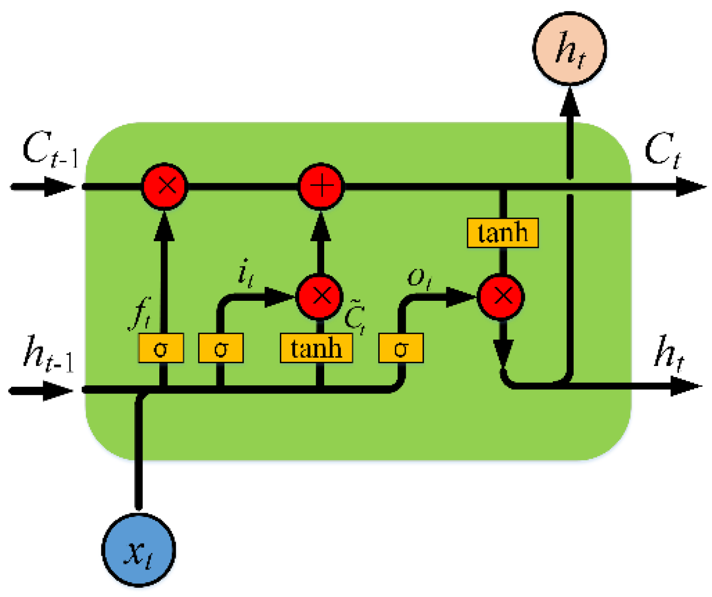
The LSTM model is the most popular in the time series domain. It was introduced by Hochreiter and Schmidhuber (1997), and was refined and popularized in subsequent work [42]. LSTM is a special kind of recurrent neural network capable of learning long-term dependencies in data. The recurring module of LSTM has a combination of four gates interacting with each other, as shown in Figure 8. A simple LSTM cell consists of four parts: forget gate, input gate, hidden cell state, and output gate.

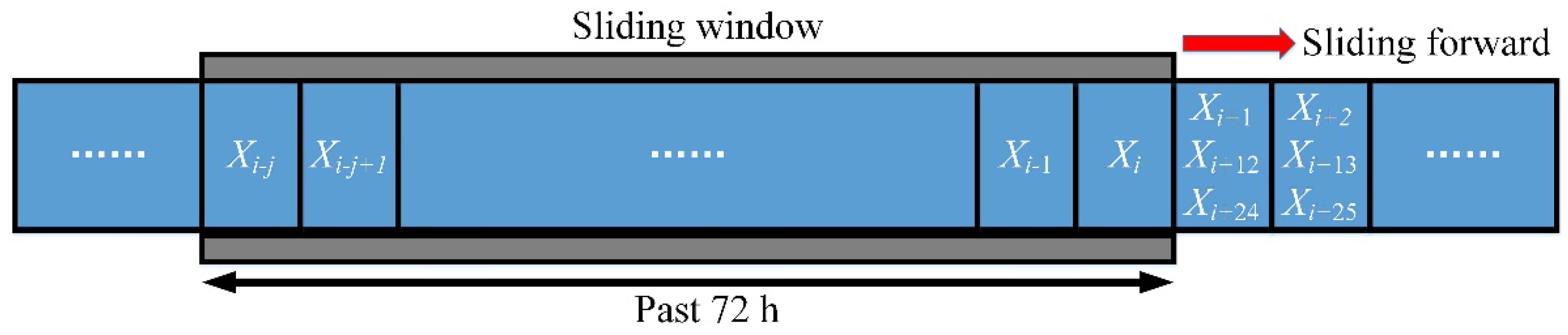
LSTM adds a dropout layer to improve the generalization ability of the algorithm. We set dropout and recurrent dropout to 0.2 and 0.5, respectively. In the LSTM calculation process, the time in the sliding window is set to the past 72 consecutive hours. The sliding window corresponding to LSTM is shown in Figure 6.

In LSTM, the building energy consumption data from 2016 and 2017 are the training dataset, and the building energy consumption data in 2018 are the test data. There are 17,451 training samples and 8760 testing samples in LSTM.

3.4. Period-Based Neural Network

LSTM is a general algorithm for solving time series problems, with the advantages of a wide application range and accurate calculation results. It is demonstrated in Section 2 that building energy consumption is periodic. When solving the energy consumption prediction problem, LSTM does not take full advantage of the inherent characteristics of such problems. This leads to too many model parameters, long calculation time, and easy overfitting when solving the energy consumption prediction problem based on LSTM.

We propose a period-based neural network algorithm to solve the problem of building energy consumption prediction. PBNN mainly improves the accuracy of building energy consumption prediction from the data structure perspective. We propose a novel sliding window structure, as shown in Figure 7, which takes advantage of the periodicity of building energy consumption. New computational methods reduce the model training and application time.

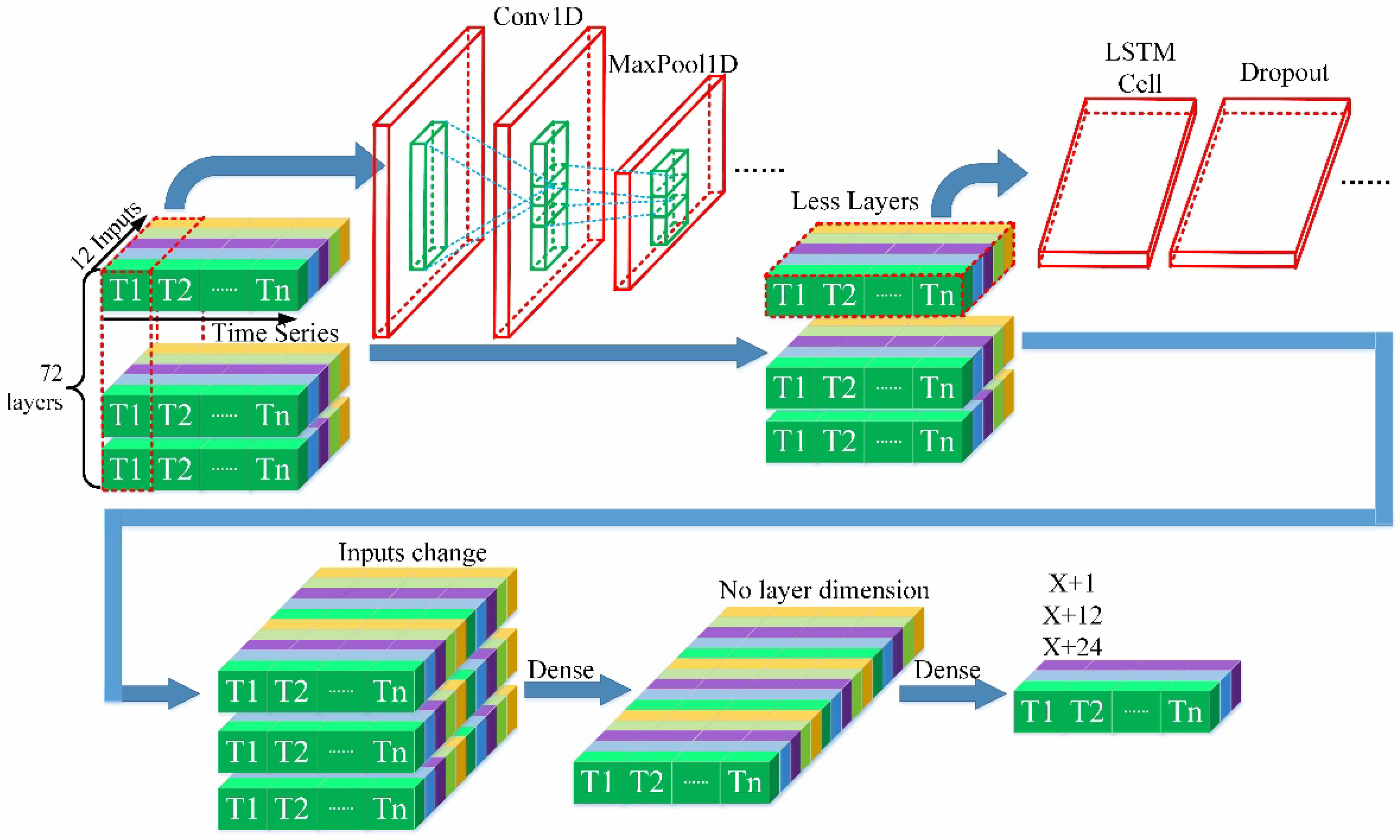
The entire framework of the PBNN is shown in Figure 9. Two main modules, CNN and LSTM, are cascaded together in this system. The CNN layer is an in-depth feature extractor that integrates periodic information on building energy consumption with lower dimensionality than the original tensor. LSTM layers extract and learn temporal features of multivariate energy consumption time series. The three-dimensional (3D) tensor is input into the PBNN model. The three dimensions of the tensor are features (12 inputs in the figure), sliding window size (72 layers in the figure), and time span (time series in the figure).

CNN consists of one-dimensional (1D) convolutional layers, ReLU layers, and 1D pooling layers. Each convolutional neuron only processes the energy consumption data of the receptive field. CNN has two significant features: local perception and parameter sharing. Time series data with periodicity satisfy the above characteristics. Therefore, the CNN introduced in the model improves the accuracy of building energy consumption prediction. The kernel size of the CNN is determined by the period of the data.

The pooling layer adopts the max-pooling method, and reduces the capacity of the model in order to reduce the number of parameters and the computational cost of the network while reducing overfitting.

LSTM is the lower layer of the PBNN, which further extracts building energy consumption information extracted by the CNN. The LSTM algorithm was introduced in more detail in the previous section.

Adam is the optimizer for this model. The loss function is the mean squared error (MSE) of the predicted and actual energy consumption.

In PBNN, the data span a period of over a year in the sliding window. The building energy consumption data from 2016 and 2017 are training datasets, and the building energy consumption data from 2017 and 2018 are test data. While the data from 2017 and 2018 are test data, only the 2018 building energy consumption is forecast. There are 8761 training samples and 8737 testing samples in PBNN.

In the 1D CNN module, the kernel size is set to 12 based on hyperparameter grid search. The choice of hyperparameters is presented in Section 3.7. The activation function is ReLU, and the padding method is set to causal. The pool size of Layer MaxPool1D is 2.

The LSTM module’s dropout and recurrent dropout are 0.2 and 0.5, respectively. The activation function is ReLU.

The batch size of the model is set to 32, and the number of training epochs is 50. An early stopping technique is introduced to reduce overfitting. The patience of early stopping is set to 4. The LSTM’s monitor is a validation loss.

In this paper, there are four main methods to address the overfitting problem:

1.

Sliding windows are introduced into energy consumption prediction to better obtain the information in the time-series data. In particular, the improved sliding window in discontinuous time can further alleviate the problem of overfitting.

2.

Periodic features are preprocessed by trigonometric and linear transformations. After preprocessing, the need for data volume is reduced in the energy consumption prediction problem.

3.

Better model hyperparameters are chosen according to the periodicity of building energy consumption. The CNN-LSTM model has fewer parameters than the LSTM model, which controls the model’s capacity.

4.

Some conventional anti-overfitting methods are introduced into training, such as adding multiple dropouts, weight sharing in CNN, and early stopping.

3.5. Traditional Sliding Window PBNN

To better verify the effect of the sliding window proposed in this paper, the traditional sliding window PBNN is also constructed. The model structures of TSW-PBNN and PBNN are the same. The main difference between them is that the two sliding windows are different. The sliding window for the TSW-PBNN is shown in Figure 6. Furthermore, the time in the sliding window is continuous.

3.6. Evaluation Criteria

To evaluate the energy prediction errors of the baseline model, LSTM, TSW-PBNN and PBNN, mean absolute error (MAE), root mean square error (RMSE), and coefficient of determination (R2) are introduced in this paper [43]. MAE focuses on the relative error, and RMSE focuses on the error. R2 measures the strength of the relationship between the model and the dependent variable on a convenient 0–100% scale. The three evaluation criteria evaluate the effect of building energy consumption prediction from three different perspectives.

$$\mathrm{MAE}=\frac{1}{N}{\displaystyle \sum _{i=1}^N\left|X_i-{\widehat{X}}_i\right|}$$

(6)

$$\mathrm{RMSE}=\sqrt{\frac{1}{N}{\displaystyle \sum _{i=1}^N{\left(X_i-{\widehat{X}}_i\right)}^2}}$$

(7)

$$R^2=1-\frac{{\displaystyle {\sum }_{i=1}^n{\left(X_i-{\widehat{X}}_i\right)}^2}}{{\displaystyle {\sum }_{i=1}^n{\left(X_i-{\overline{X}}_i\right)}^2}}$$

(8)

where X_i is a vector representing N actual values, ${\widehat{X}}_i$ is a vector representing N prediction values, ${\overline{X}}_i$ represents the mean of the true values, and n is the number of timestamps in the test series.

3.7. Hyperparameter Optimization

Hyperparameter optimization can avoid both the overfitting and underfitting of the model. Moreover, hyperparameter optimization helps deep learning models to generalize well. Generalization refers to the ability of a model to perform well on both training data and new data. Since the model’s performance varies with the hyperparameters, it is essential to set them appropriately.

Grid search determines a set of values for each hyperparameter, runs the model with each possible combination of these values, and selects the values that produce the best results. Grid search involves guesswork since the values to be tried are set manually by the algorithm designer [44].

We performed a grid search on hyperparameters in LSTM and PBNN. The search range of LSTM model hyperparameters is shown in

Table 2. Hyperparameter grid search for LSTMs.

Hyperparameter	Implication	Range
LSTMLayers	LSTM layer repetitions	[1, 2, 3, 4]
LSTMUnits	LSTM capacity	[5, 10, 100, 300]

. The search objective is to minimize the average building energy consumption MAE in the next 1 h, 12 h, and 24 h. The calculation results show that the energy consumption prediction MAE of the LSTM model is the smallest when LSTMLayers is 2, LSTMUnits is 300, and the average MAE is 14.04%.

PBNN is more complex than LSTM. Therefore, it contains more hyperparameters. The search range of hyperparameters of the PBNN model is shown in

Table 3. Hyperparameter grid search for PBNNs.

Hyperparameter	Implication	Range
ConvLayers	Convolutional layer repetitions	[1, 2, 3, 4]
kernelSize	Convolution size	[2, 12, 24]
filters	The number of different convolution kernels	[5, 10, 50, 100]
LSTMLayers	LSTM layer repetitions	[1, 2, 3, 4]
LSTMUnits	LSTM capacity	[5, 10, 100, 300]

. The calculation results show that the energy consumption prediction MAE of the PBNN is the smallest when [ConvLayers, kernelSize, filters, LSTMLayers, LSTMUnits] is [2, 12, 5, 1, 100], and the average MAE is 10.31%. The optimal scale of the convolution kernel is 12, which implies that the building energy consumption data have a periodicity of 12 h. This result verifies the previous conclusions obtained by the Fourier transform. The hyperparameters of TSW-PBNN are the same as those of PBNN.

4. Results and Discussion

This section compares the performance of LSTM, TSW-PBNN, and PBNN sequentially from the perspectives of model prediction error, model computation time, stability, robustness, and feature processing. Finally, two new buildings are selected to demonstrate the PBNN prediction performance under different scenarios.

4.1. Model Prediction Errors

The prediction results of the baseline model, LSTM, TSW-PBNN, and PBNN are shown in

Table 4. Comparison of prediction errors of the baseline model, LSTM, TSW-PBNN, and PBNN.

Time Horizon	Model	MAE(%)	RMSE	R2
1 h	Baseline	24.44	39.33	0.29
	LSTM	13.78	19.17	0.74
	TSW-PBNN	11.90	16.53	0.72
	PBNN	9.60	16.24	0.84
12 h	Baseline	24.44	39.33	0.29
	LSTM	14.64	20.91	0.68
	TSW-PBNN	14.25	19.09	0.67
	PBNN	10.78	17.58	0.81
24 h	Baseline	24.44	39.33	0.29
	LSTM	13.69	19.99	0.72
	TSW-PBNN	14.22	18.68	0.69
	PBNN	10.56	18.08	0.78

. In MAE, RMSE, and R2, the prediction results of LSTM, TSW-PBNN, and PBNN are significantly better than those of the baseline model. This shows that complex neural network algorithms can improve the energy consumption prediction results. When predicting the building energy consumption for the next 1 h, the PBNN prediction error is 9.6%, which is 4.18% smaller than the LSTM prediction error. In the calculation results of RMSE, the energy consumption prediction bias of PBNN is 2.93 kWh lower than that of LSTM. The MAE of PBNN is 2.30%, 3.47%, and 3.66% lower than that of TSW-PBNN when predicting energy consumption for 1 h, 12 h, and 24 h in the future, respectively. By comparing the prediction results of TSW-PBNN and PBNN, the sliding window proposed in this paper is found to be superior to the traditional continuous-time sliding window. After adopting the PBNN model, the independent variable explained 84% of the dependent variable, which was 10% higher than the corresponding value in LSTM. For predicting building energy consumption in the next 12 h and 24 h, the R2 of PBNN is 0.14 and 0.09 greater than that of TSW-PBNN, respectively. PBNN outperforms LSTM and TSW-PBNN in all of the evaluation criteria of the prediction results.

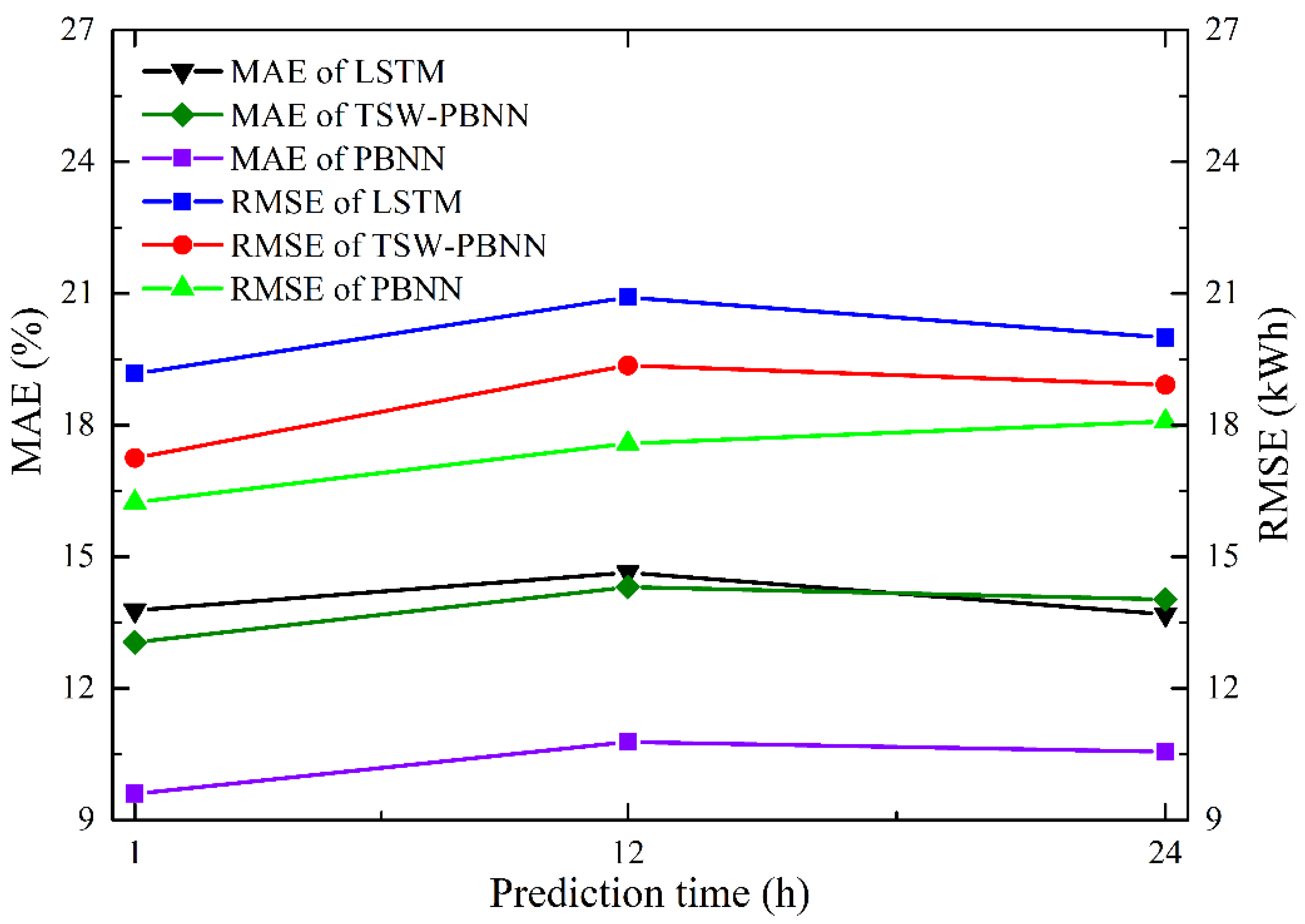
Since the baseline model is just a simple persistence model, it performs the same in predicting building energy consumption for the next 1 h, 12 h, and 24 h. Figure 10 shows the performance of LSTM, TSW-PBNN, and PBNN in predicting different moments in the future. In PBNN, the MAEs of energy consumption in the next 1 h, 12 h, and 24 h are 9.60%, 10.78%, and 10.56%, respectively. The energy consumption prediction error for the next 1 h is the smallest. The energy consumption predictions for the next 12 and 24 h are relatively close. The calculation results of the other five groups are similar to the above conclusions. As the prediction time becomes longer, the prediction error tends to increase. However, this trend is not always the case. The inherent periodicity of energy consumption data may make predictions more accurate at certain times. Under the same conditions, the error of the PBNN prediction results is smaller than that of the LSTM and TSW-PBNN prediction results.

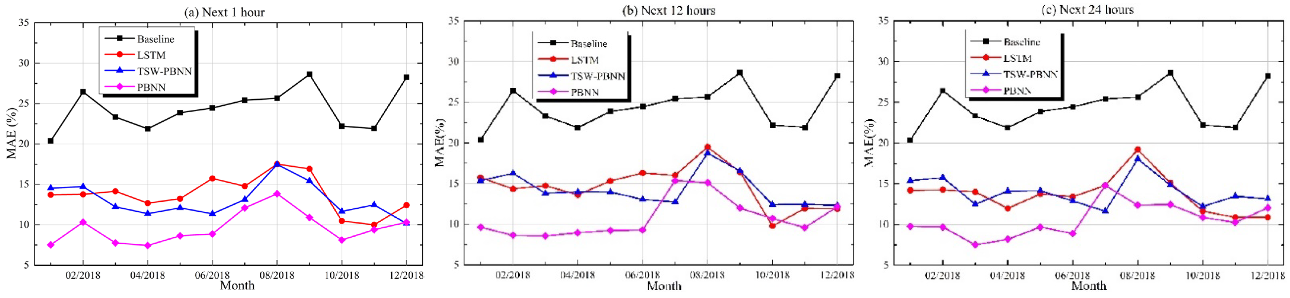
Table 4 shows the errors of these models in the energy consumption prediction for the whole year of 2018. The prediction results for the entire year are decomposed by month in order to obtain the prediction results of energy consumption for each month. The monthly energy consumption prediction is compared with the ground truth of each month. Then, the prediction errors for each month are obtained. The predicted performances per month of the baseline model, LSTM, TSW-PBNN, and PBNN are shown in Figure 11.

In most cases, the MAE of PBNN is the smallest, followed by TSW-PBNN and LSTM. The MAE of the baseline model is the largest. There are the following error trends in the prediction results of LSTM, TSW-PBNN, and PBNN. The MAE in January, February, and March is the average MAE for the whole year. MAE decreases in April, and increases slightly in May and June. MAEs in July, August, and September are significantly higher than the average MAE. The MAE in October hits rock bottom before increasing again in November and December.

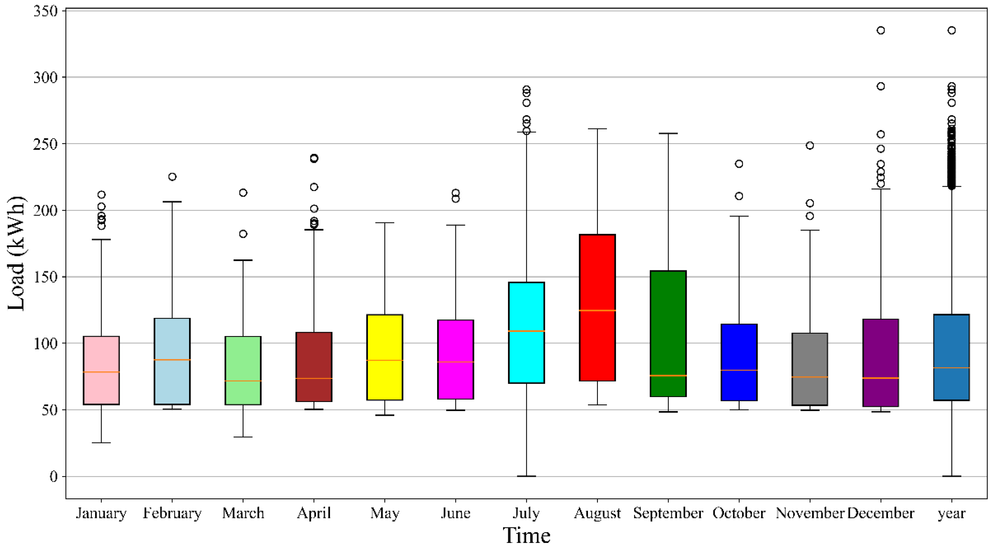
To explain the above trends, we made a box plot of energy consumption for each month and the entire year in 2018, as shown in Figure 12. The bottom 25%, the median, and the top 25% of the annual energy consumption ground truth, excluding outliers, are 57.11 kWh, 81.47 kWh, and 121.50 kWh, respectively. The same April energy consumption ground truths are 56.16 kWh, 73.55 kWh, and 108.05 kWh. The same October energy consumption ground truths are 56.73 kWh, 79.76 kWh, and 114.20 kWh. The bottom 25%, the median, and the top 25% of the August energy consumption ground truth are 56.73 kWh, 79.76 kWh, and 114.20 kWh, respectively.

The distribution of energy consumption data in April and October is the closest to the distribution of energy consumption data for the whole year. The energy consumption in August is significantly higher than the average energy consumption for the entire year. At the same time, April and October have the most petite MAEs, whereas the MAE is the largest in August. Comparing Figure 11 and Figure 12, the more similar the distribution of energy consumption data in a month and the distribution of energy consumption data in the entire year are, the smaller the MAE of that month is. By separately training a small neural network model on the energy consumption data of the third quarter (Q3), we can reduce the overfitting of the neural network. The model prediction error can be significantly reduced by introducing two PBNNs (one PBNN for Q3 and one PBNN at other times). From Figure 12, the minimum energy consumption in July is 0 kWh. By detecting the energy consumption data, the energy meter reading at 2018/7/14 6:00:00 is 0. The data before and after this time are standard. Therefore, the energy meter reading at this moment is wrong. We do not pursue the minimum prediction error, so the reading of the energy meter at this moment is not modified.

4.2. Model Computation Time

The experimental computing platform in the paper is an Intel^® Core™ i9-10850K CPU @3.60 GHz CPU, RAM 64 GB, Windows 10 64 bit, NVIDIA GeForce RTX 3090, Python 3.8, and TensorFlow 2.3.

In addition to model prediction accuracy, model computation time is another dimension of evaluating models. In neural network applications, model computing time is divided into training and inference time. Training time is generally several hours or even days, and requires powerful GPUs, which increases training costs and power consumption. This will also indirectly limit the extent of hyperparameter tuning and model training. Inference time is crucial in determining whether the model can be run online. PBNN has a more complex structure and more hyperparameters than LSTM. However, this does not mean PBNN takes a long time to train and test, as shown in

Table 5. Computation time of LSTM, TSW-PBNN, and PBNN.

Model	Training Samples	Training Time	Inference Time
LSTM	17,451	4528 s	1.19 ms
TSW-PBNN	17,451	787 s	0.42 ms
PBNN	8761	483 s	0.66 ms

. Since there is a max-pooling layer in the CNN layer, the data are compressed when they pass through the CNN and enter the LSTM. This results in a practically smaller capacity of the PBNN model, thereby reducing the training time. Due to the different sliding window structures, the training samples of LSTM or TSW-PBNN are almost twice those of PBNN. The training time of PBNN is approximately half that of TSW-PBNN.

PBNN has fewer parameters, which can reduce inference time. However, the sliding window of PBNN is more complicated and requires more computation time. The inference time of PBNN is longer than that of TSW-PBNN. Overall, the inference times of TSW-PBNN and PBNN are not significantly different. The inference times of the three models are at the millisecond level, which can meet the requirements of online computing.

4.3. Stability of Model Prediction

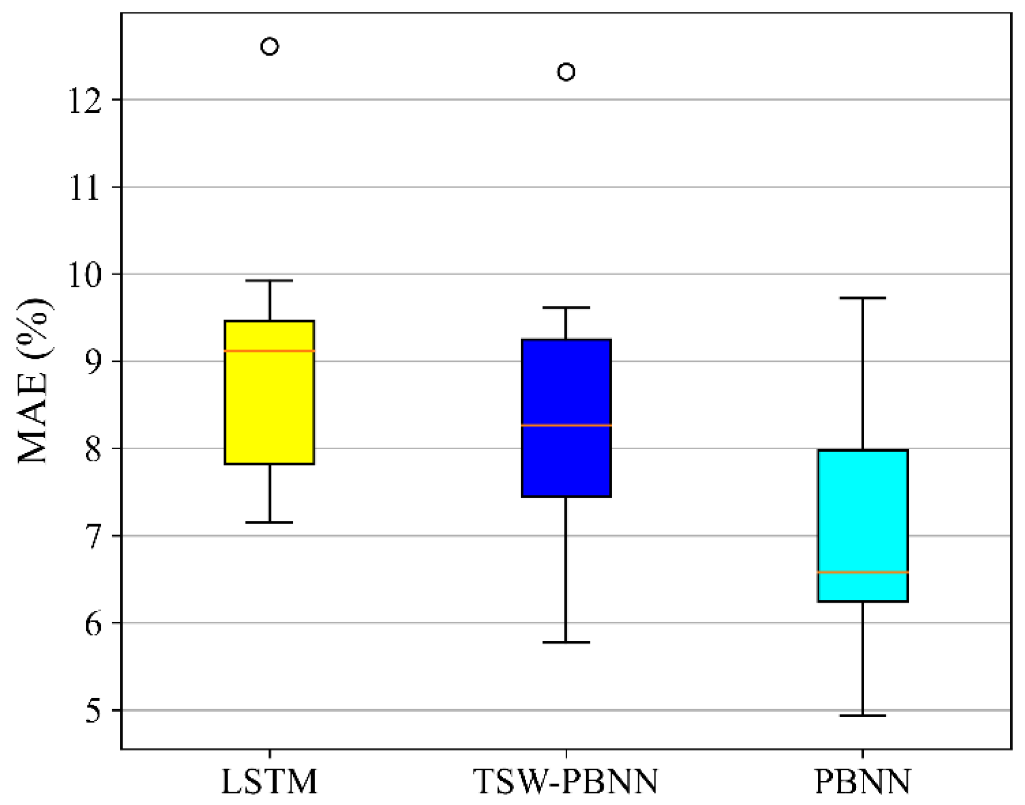
The calculation result of the neural network algorithm is random. The choice of dataset will also affect the accuracy of the neural network algorithm. Twelve-fold cross-validation was performed on the entire dataset. The MAE distribution of energy consumption prediction in the next 24 h is shown in Figure 13. Three-quarters of the MAEs trained by PBNN are less than 8%. Approximately one-quarter of the MAEs trained by LSTM are less than 8%. In most cases, the prediction error of PBNN will be minor. The standard deviations of LSTM, TSW-PBNN, and PBNN are 1.50, 1.65, and 1.36, respectively. PBNN calculation results are more stable. There are outliers in LSTM and TSW-PBNN, which can be recognized as failure cases.

Training is often terminated early in these cases, after approximately ten training rounds. Due to insufficient training, the energy consumption prediction error of the trained model is abnormally large. The initialization parameters of the neural network are random, so each training is not the same. However, PBNN rarely has insufficient training rounds. PBNN is less affected by random initialization parameters.

4.4. The Robustness of LSTM, TSW-PBNN, and PBNN

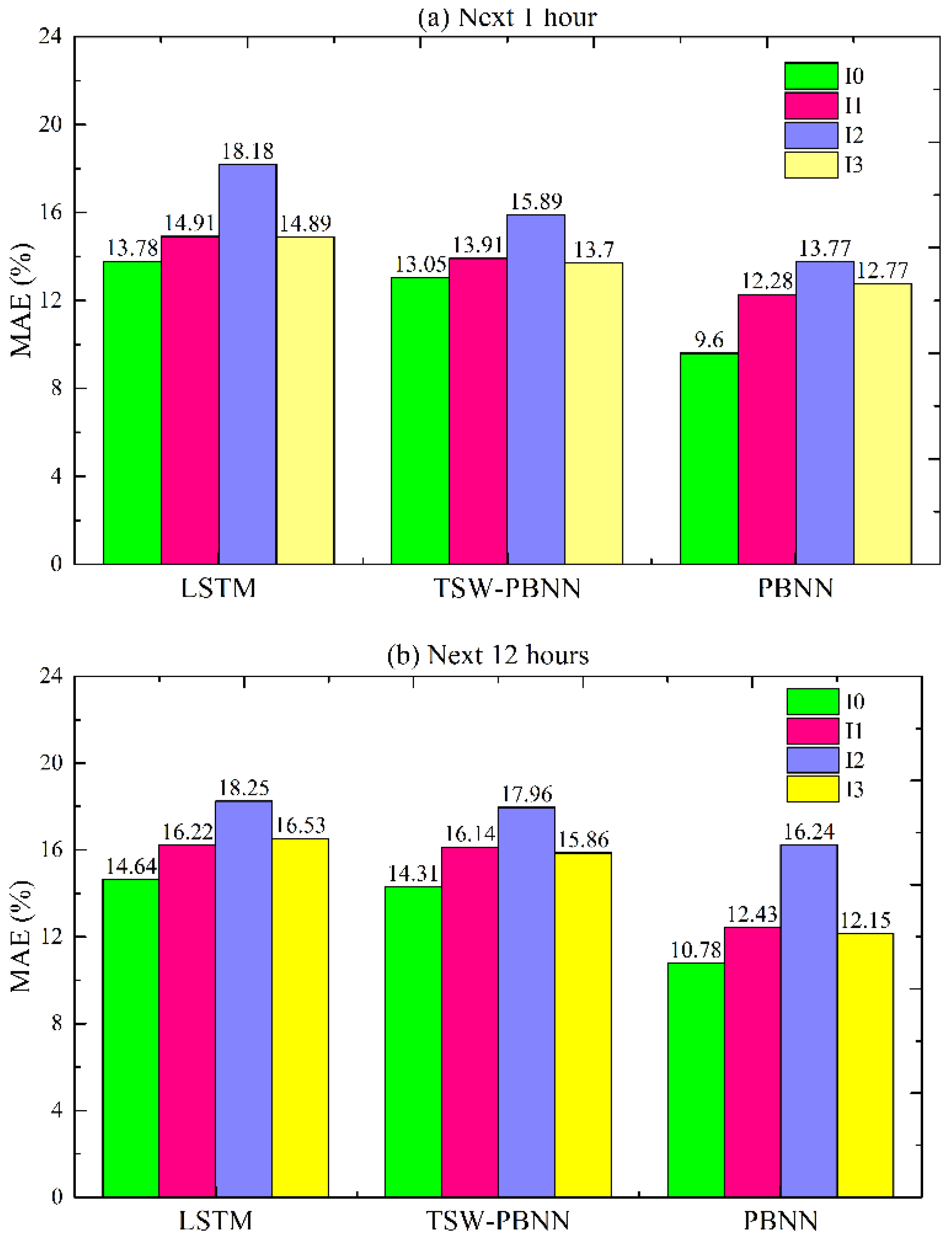
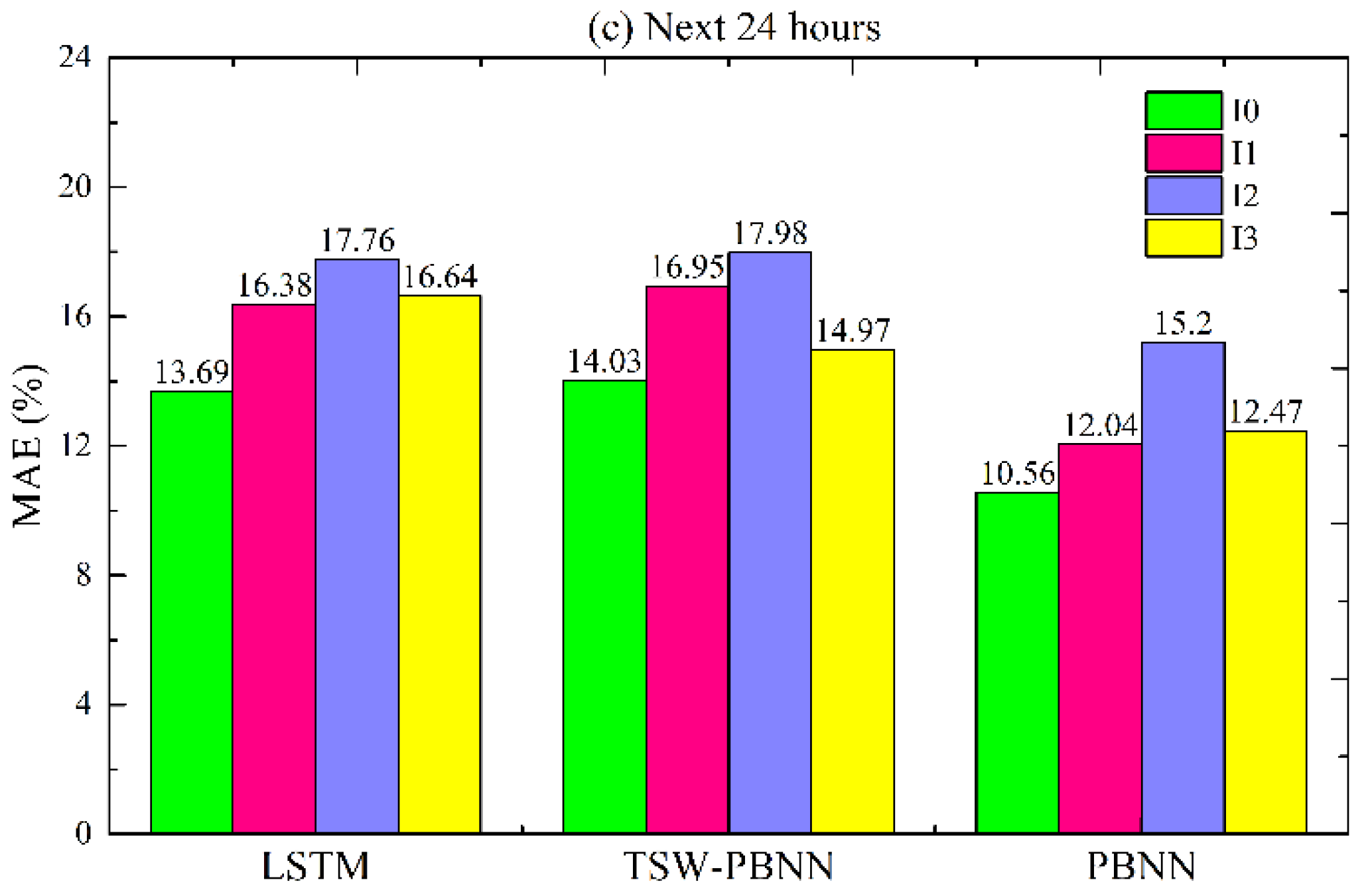
In engineering problems, the amount of training data needed to meet the requirements of neural network algorithms is often challenging. A more extensive training sample size means a higher cost. Sometimes, to reduce costs, it is acceptable to reduce the accuracy of the predictive model due to insufficient training samples. To study the robustness of the model in terms of the amount of training data, we divided the training data into four groups, “I0” to “I3”. I0 contains four quarters’ data, and I3 only holds information for the fourth quarter. Since the sliding window of PBNN requires the same period as the previous year, the test data can only maintain the same period as the training data. The final test data for LSTM, TSW-PBNN, and PBNN are divided into the same four groups. The periods for the input data are shown in

Table 6. Composition of different training data.

Input No.	Training Data Length	Period of Data
I0	100% training dataset	Q1, Q2, Q3, Q4
I1	75% training dataset	Q2, Q3, Q4
I2	50% training dataset	Q3, Q4
I3	25% training dataset	Q4

.

Figure 14 shows the MAEs of the LSTM, TSW-PBNN, and PBNN under different input choices. Compared with I0, I1, and I3, the MAE gradually increases with the decrease in training data. In Figure 14c, the MAE of LSTM increases from 13.69% to 16.64% compared with I0 and I3. The MAE of PBNN increases from 10.56% to 12.47%. Energy consumption prediction errors do not increase significantly.

Compared with I2 and I3, the training error is reduced when the amount of training data is reduced. The period for the test data for I2 is Q3 and Q4. The period for I3 is Q4. The calculation results imply that building energy consumption data in Q3 (corresponding to July, August, and September) are difficult to predict. The energy prediction error metrics of LSTM, TSW-PBNN, and PBNN will decrease if Q3 data are discarded. However, the above strategy falls into the “survivor bias” trap. We need to collect more Q3 building energy consumption data to make the model more robust.

4.5. Preprocessing of Periodic Features

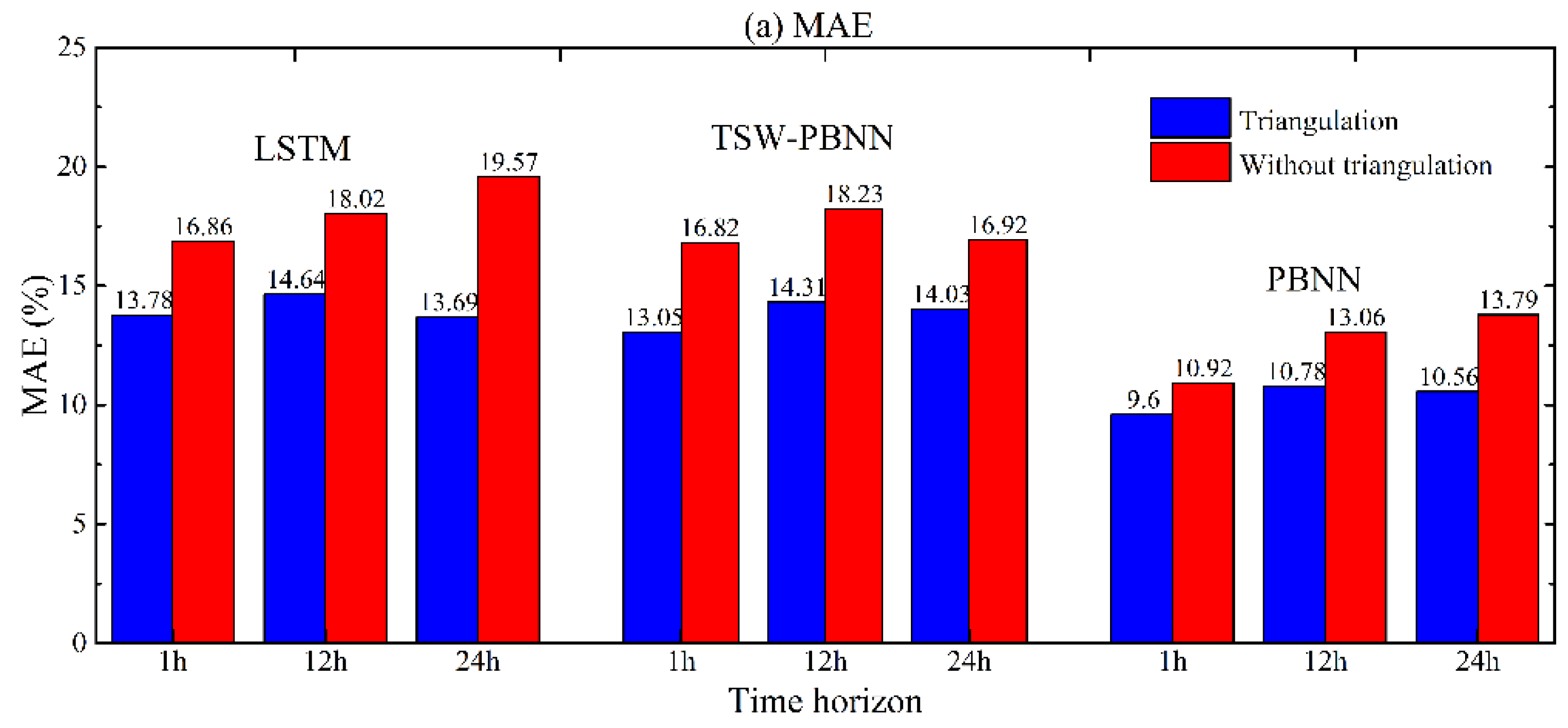
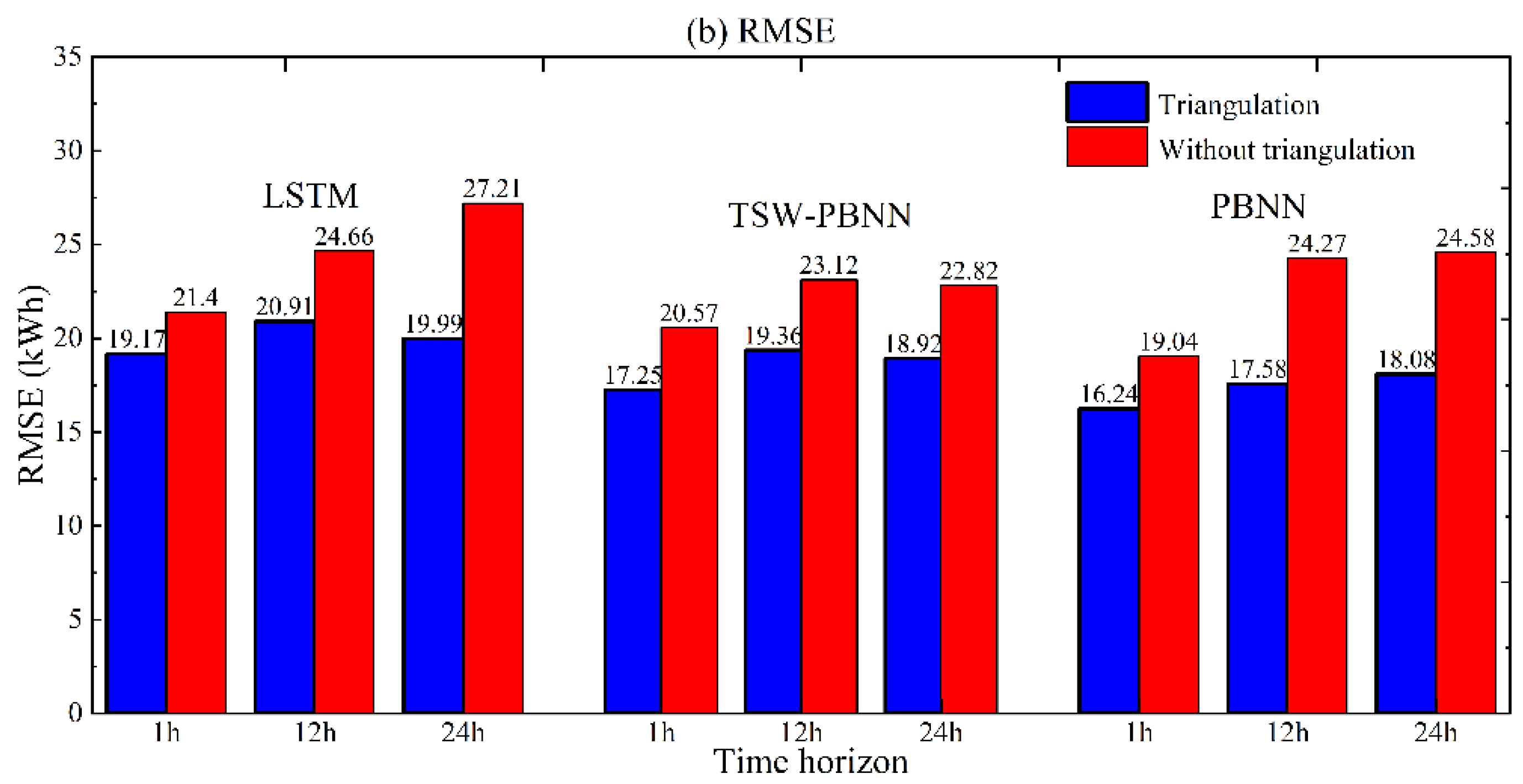
In Section 3.1, Equation (3) is used to perform trigonometric function preprocessing on periodic and discrete features. Here, the energy consumption models are trained separately based on the features preprocessed by the trigonometric function and the original features. The energy consumption prediction errors of these models after training are shown in Figure 15. The energy consumption prediction error of LSTM with triangulation preprocessing is, on average, 4.11% lower than that without triangulation preprocessing. The average energy consumption prediction error of PBNN can be reduced by 2.28% through trigonometric function preprocessing. The calculation conclusion of the TSW-PBNN is similar to that of the PBNN. From the perspective of RMSE, trigonometric function preprocessing can reduce the energy consumption prediction errors of LSTM, TSW-PBNN, and PBNN by 4.40 kWh, 3.66 kWh, and 5.33 kWh, respectively. As the prediction time horizon increases, the energy consumption prediction errors of the model trained on the original features increase rapidly.

It is generally believed that a significant advantage of neural networks over shallow machine learning is that manual feature engineering is not needed. However, the prediction accuracy can be significantly improved after feature engineering is adopted in predicting building energy consumption. This contradiction is mainly due to the number of training samples. In engineering, general computing tasks cannot provide sufficient and valid training data. In the case of limited data, feature engineering is necessary. Deep learning cannot wholly change the above facts. However, in the engineering field, deep learning can reduce the importance of feature engineering. At the same time, a more sophisticated network architecture design can reduce overfitting, the number of parameters, and the dependence on feature engineering.

4.6. Model Performance under Different Scenarios

We selected Building 164 and Building 230 from the GEPIII competition data for a comparative study of LSTM, TSW-PBNN, and PBNN. The basic information of Building 164 and Building 230 is shown in

Table 7. The basic information of Building 164 and Building 230.

Building Id	Primary Use	Square (Feet)	Year Built	Floor Count
164	Warehouse/storage	12,908	1979	2
230	Education	10,334	/	2

. The primary use of Building 164 is as a warehouse/storage. The energy consumption of the warehouse is relatively less disturbed by human work and rest. The primary use of Building 230 is education, as is the primary use of Building 185. The construction year for Building 230 is missing. All data in this subsection are available from the website [37].

The prediction errors of the baseline model, LSTM, TSW-PBNN, and PBNN for Buildings 164 and 230 are shown in

Table 8. Energy consumption prediction error of Building 164.

Time Horizon	Model	MAE (%)	RMSE	R2
1 h	Baseline	22.85	15.14	0.51
	LSTM	16.73	10.92	0.69
	TSW-PBNN	14.99	9.25	0.77
	PBNN	15.13	9.88	0.75
12 h	Baseline	22.85	15.14	0.51
	LSTM	17.20	11.92	0.66
	TSW-PBNN	15.87	10.37	0.72
	PBNN	15.77	10.41	0.73
24 h	Baseline	22.85	15.14	0.51
	LSTM	17.08	11.77	0.66
	TSW-PBNN	15.34	9.93	0.76
	PBNN	15.06	9.78	0.78

and

Table 9. Energy consumption prediction error of Building 230.

Time Horizon	Model	MAE (%)	RMSE	R2
1 h	Baseline	33.81	7.95	0.61
	LSTM	19.21	5.02	0.77
	TSW-PBNN	17.13	4.19	0.82
	PBNN	14.44	3.57	0.87
12 h	Baseline	33.81	7.95	0.61
	LSTM	20.32	5.13	0.75
	TSW-PBNN	17.64	4.45	0.81
	PBNN	14.90	3.88	0.84
24 h	Baseline	33.81	7.95	0.61
	LSTM	20.26	5.17	0.74
	TSW-PBNN	17.42	4.32	0.82
	PBNN	14.73	3.81	0.85

, respectively. In Table 8, the baseline model still performs the worst. However, it is not much worse than that predicted by the other models. The prediction results of TSW-PBNN and PBNN are close, and both are better than LSTM. When predicting the energy consumption in the next 24 h, the prediction error of PBNN is smaller than that of TSW-PBNN. In this case, the traditional sliding window and the time-discontinuous sliding window behave similarly. This does not reflect the superiority of the time-discontinuous sliding window. The energy consumption of the warehouse is relatively stable, and its daily, weekly, and annual periodic characteristics are not obvious. In this situation, the persistence model will perform relatively well.

In Table 9, PBNN shows a significantly superior performance. When predicting energy consumption in the next 24 h, the MAE of PBNN is 19.08%, 5.53%, and 2.69% lower than that of the baseline model, LSTM, and TSW-PBNN, respectively. The analysis results for Buildings 185 and 230 were similar. Buildings 185 and 230 serve the same primary use. Their periodic characteristics are relatively strong. In this scenario, the model based on the time-discontinuous sliding window makes better predictions.

5. Conclusions

Accurate building energy consumption prediction can provide the basis for DH regulation from the feedback mode to the feedforward mode. Feedforward regulation can improve the operating efficiency of the DH, thereby achieving energy savings and consumption reduction. To better predict building energy consumption, we propose a PBNN model. PBNN exploits periodicity in three directions to improve energy consumption prediction. PBNN reflects periodicity from three directions. According to the periodicity of energy consumption data, the sliding window consists of the past 24 h, 24 h in the past week, and 24 h in the past year. For periodic and discrete features such as wind direction and hour, these features are transformed by trigonometric functions. These features are then linearly transformed to finally obtain features in the [0, 1] interval. The CNN layer is added before the data enter the LSTM layer. The convolution kernel scale of CNN is set to 12 according to the period of energy consumption data.

In this study, LSTM, TSW-PBNN, and PBNN are introduced to predict the building energy consumption. Important results are summarized as follows:

1.

According to the unique periodicity of energy consumption data, a sliding window integrating daily, weekly, and annual cycle information is proposed. The effectiveness of this sliding window is demonstrated by comparing LSTM, TSW-PBNN, and PBNN.

2.

PBNN outperforms LSTM and TSW-PBNN on MAE, RMSE, and R2. The training time of PBNN is approximately one-tenth of that of LSTM or half that of TSW-PBNN. PBNN drastically reduces model computation time.

3.

When the energy consumption distribution of the month deviates from the energy consumption distribution of the whole year, the energy consumption prediction error of the month is large. The energy consumption in July, August, and September is significantly higher than the annual average energy consumption. These three months have the largest error in terms of energy consumption predictions.

4.

For buildings with significant periodic characteristics, PBNN has obvious advantages. PBNN performs well when the primary use of the building is education. The time-discontinuous sliding window does not help energy consumption prediction when the primary use of the building is as a warehouse.