Influence of the Gas Model on the Performance and Flow Field Prediction of a Gas–Liquid Two-Phase Hydraulic Turbine

Abstract

A two-phase hydraulic turbine’s performance and flow field were predicted under different Inlet Gas Volume Fractions (IGVF) with incompressible and compressible models, respectively. The calculation equation of equivalent head, hydraulic efficiency, and flow loss considering the expanding work of compressible gas were deduced based on the energy conservation equations. Then, the incompressible and compressible results, including the output power and flow fields, are compared and analyzed. The compressible gas model’s equivalent head, output power, and flow loss are higher than the incompressible model, but the hydraulic efficiency is lower. As the IGVF increases, the gas gradually diffuses from the blade’s working surface to its suction surface. The gas–liquid separation happens at the runner outlet in the compressible results due to the gas expansion. The area of the low-pressure zone in the incompressible results increases with the IGVF. However, it decreases with the IGVF in the compressible results. As the gas expands in the blade passage, it takes up more flow area, causing the high liquid velocity in the same passage. The runner’s inlet gas distribution affects the liquid flow angle, causing the inlet shock and high TKE areas, especially in the blade passage near the volute tongue. The high TKE area in the compressible results is larger than the incompressible results because the inlet impact loss and the liquid velocity in the blade passage are higher. This paper provides a reference for selecting gas models in the numerical simulation of two-phase hydraulic turbines.

1. Introduction

Hydraulic turbines can be used as a device to recover the residual pressure energy of the pressurized liquid. It is widely used in the petrochemical industry, ammonia synthesis of chemical fertilizer, purification of liquid natural gas, and other fields [1,2,3]. However, in some special working conditions, the fluid at the inlet of the hydraulic turbine will contain an amount of gas, which significantly reduces its hydraulic efficiency and flow stability.

Many researchers [4,5,6,7] have studied the gas–liquid two-phase flow problem of the pump or Pump as Turbines (PATs). Sun [8,9] investigated the inter-blade cavitation vortex in a Francis turbine using the mixture multiphase model and verified the simulation results with hydraulic efficiency and visualization figures. As the vapor volume fraction induced by the cavitation was low, the compressibility of vapor was neglected. Huang [10], Caridad [11], and Suh [12] used the Eulerian–Eulerian multiphase flow model to establish numerical pump models under the gas–liquid two-phase condition and verified the model’s accuracy through a pump performance test. Zhang et al. [13,14] studied the flow field characteristics in a multiphase pump under different inlet GVFs. The research indicated that the gas phase was mainly concentrated near the hub at the impeller outlet; the degree of aggregation and the gas inhomogeneity increased as the IGVF increased. When the IGVF is 21%, the gas phase in the impeller accumulated obviously and extended to the suction surface of the guide vane inlet. Ge et al. [15] adopted the CFD-PBM (CFD-Population Balance Model) model to study the influence of the gas phase distribution in the centrifugal pump. The results show that a large amount of gas accumulated in the impeller as the IGVF increased to a particular value, and a big air mass formed at the inlet of the impeller, leading to “Surging” of the pump. Sun [16] and Chen [17] studied the three-dimensional transient flow field in the hydraulic turbine, which was designed based on the model of the micro Francis turbine. They found that the power and efficiency of the hydraulic turbine gradually decreased with the IGVF. The area of low pressure increased with the IGVF while the pressure difference between the pressure surface and the suction surface of the blade decreased. Kim [18] analyzed the accuracy of the multiphase models by comparing the simulation and experimental results and indicated that the Grace model has the highest reliability.

The above studies all assumed that the gas is incompressible. When the IGVF was low and the pressure difference between inlet and outlet was small, the gas phase density changed little, which made it reasonable to consider the gas incompressible. However, when the IGVF was high and the pressure difference between inlet and outlet was large, the compressibility of the gas phase would have a significant influence on the flow field distribution and performance. Yan [19] predicted the performance of the multiphase pumps using the ideal gas compressible model. The final simulation results were in good agreement with the experimental results, which proved that the numerical model could accurately predict the performance of the multiphase pumps. Poullikkas [20] and Si [21] studied the two-phase flow characteristics of the centrifugal pumps, regarded the gas phase as compressible, and found that the accumulation of the gas phase in the impeller changed the liquid flow direction, reduced the flow area, and affected the energy transfer in the impeller. Shi et al. [22,23,24] simulated the two-phase flow characteristics in a PAT using the mixture multiphase and ideal gas compressible models. The results indicated that the gas reduced the homogeneity of velocity distribution in the turbine, and a low-speed zone appeared on the pressure surface of the blade, which deteriorated the stable operation of the hydraulic turbine. Shi et al. [25,26] found that a large-scale vortex appeared in the flow passage of the impeller of a PAT at an IGVF of 21%. As the IGVF increased, the hydraulic loss of each part of the turbine increased, and the impeller loss was the primary loss. Although the above research included the gas’s compressibility in their numerical models, its influence has not been analyzed and discussed. Hence, the influence of the incompressible and compressible gas models on the prediction of the flow field and performance of two-phase hydraulic turbines is still unclear at different IGVFs.

The present paper established a numerical model for a two-phase hydraulic turbine using the incompressible and compressible gas models to predict their flow field. First, the calculation equation of hydraulic efficiency and flow loss when the gas was compressible were deduced based on the conservation of energy and thermal process equations. Then, the performance, flow field, and flow loss predicted by different gas models were compared to investigate the influence of the gas model. The research provides a reference for selecting gas models in two-phase hydraulic turbines.

2. Methodology and Fundamental Equations

2.1. Physical Model Parameters

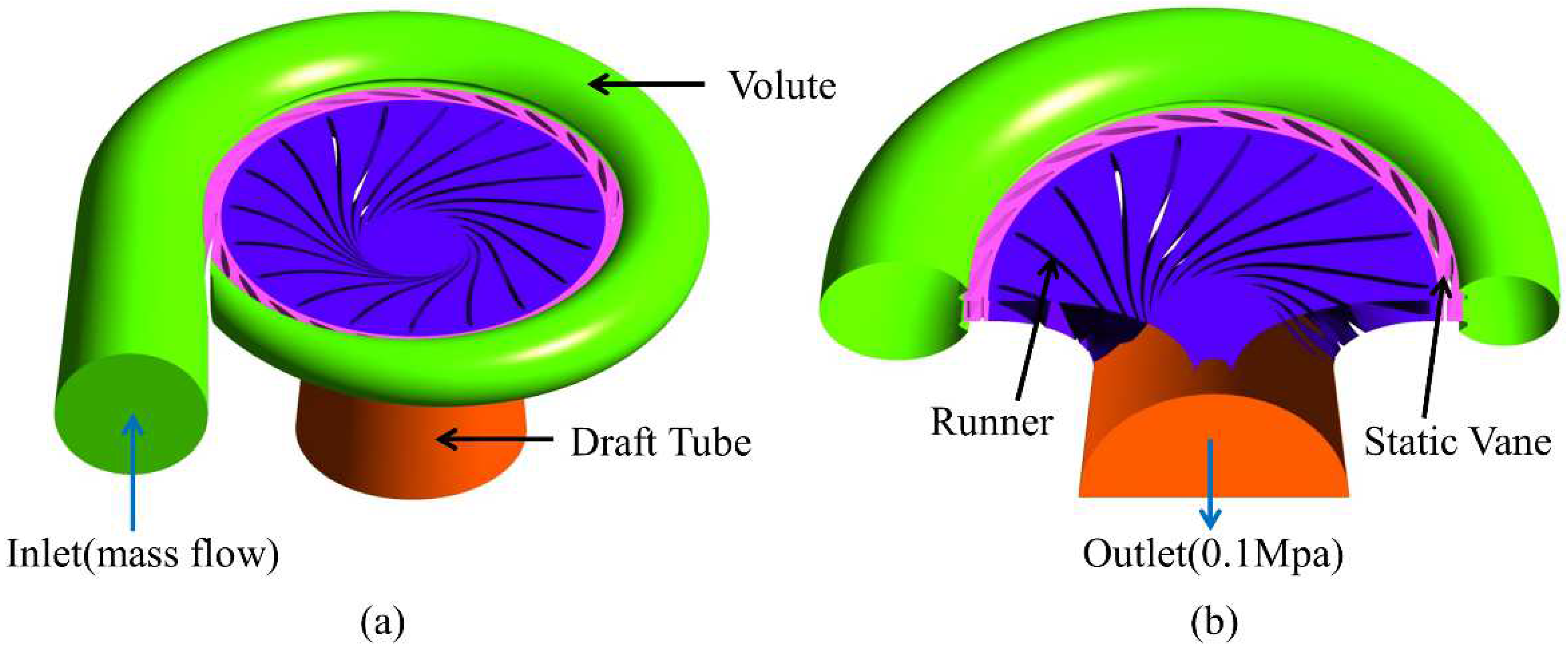
As shown in Figure 1, this paper selected a hydraulic turbine as the research object. The hydraulic turbine consists of the volute, static vane, runner, and draft tube. The parameters of the hydraulic turbine are listed in

Table 1. Design parameters of the hydraulic turbine.

Variable	Symbol	Unit	Value
Unit flow rate	Q11	L/s	350
Rated head	H	m	110
Unit speed	n11	r/min	34
Specific speed	ns	m3/4/s3/2	70
Volute inlet diameter	D	m	0.18
Runner diameter	D1	m	0.24
Draft tube outlet diameter	d	m	0.27
Static vane number	Z1	-	24
Runner number	Z2	-	19

. In this paper, the flow field and performance of the hydraulic turbine are numerically simulated using different gas models under variable IGVFs (5%, 10%, 15%, 20%).

The Equations (1) and (2) can be used to obtain the actual flow rate and actual speed:

$$Q=Q_{11}\cdot D_1^2\cdot \sqrt{H}$$

(1)

$$n=\left(n_{11}\cdot \sqrt{H}\right)/D_1$$

(2)

In Equations (1) and (2), the unit flow rate Q₁₁ and unit speed n₁₁ are the flow rate and speed when the turbine has a diameter of 1 m and a head of 1 m. They are deduced from the hydraulic similarity theory and represent the characteristic of a given type of turbine [27]. Usually, when a type of hydraulic turbine is selected, the unit values of the model turbine are given. In Table 1, the specific speed of the turbine is given, which is the rotational speed of the turbine when the turbine outputs the power of 1 kW under the head of 1 m [27]. The turbine shape could be indicated by the specific speed.

2.2. Numerical Model and Boundary Conditions

The steady numerical simulation was conducted using commercial software ANSYS CFX under two-phase working conditions. The primary phase is water, and the secondary phase is air. There are two kinds of gas models: One is the compressible model of Air Ideal Gas. The gas density in the model changes according to the following equation [28]:

$${\rho }_{g-com}=p/RT$$

(3)

The other is the incompressible model of Air at 25 ℃, where the gas density is a constant.

The Eulerian–Eulerian inhomogeneous multiphase model is adopted for the two-phase flow. In the inhomogeneous model, there are three methods to calculate the interfacial area density: the particle model, the mixture model, and the free surface model. The particle model regards gas as spherical bubbles with a mean diameter to calculate the interfacial area density [28]. The particle model is more suitable for the two-phase simulation of low gas volume fractions. In the particle model, the drag force between gas and liquid can be calculated with several models. The Grace model has good reliability [18] and is used in the simulation.

The total energy model is used for calculating the heat transfer in the simulation, which is not mentioned in many references [19,20,21,22,23,24,25,26]. It is necessary when the gas is compressible, as the gas absorbs heat when it expands. The SST k-ω turbulence model was used for the continuous phase water because it could accurately predict the flow separation induced by the turbomachine owing to blending the individual strength of the k-ε and k-ω models [8]. The turbulence model for air was the dispersed phase zero equation model. The numerical simulation convergence criterion was that the root mean square (RMS) value was lower than 10⁻⁵. The boundary condition settings are listed in

Table 2. Boundary conditions of the hydraulic turbine.

Items	Settings	Value
Inlet boundary conditions	IGVF: water mass flow (kg/s)	0%IGVF:211.0; 5%IGVF:200.5; 10%IGVF:189.9; 15%IGVF:179.4; 20%IGVF:168.8
Outlet boundary condition	static pressure (MPa)	0.1
Wall boundary conditions for water	no-slip wall	-
Wall boundary condition for gas	free-slip wall	-
Interface between the static vane and runner	frozen rotor	-

. The IGVF changes from 0 to 20% when the inlet water mass flow rate changes from 211.0 kg/s to 168.8 kg/s.

2.3. Mesh Generation and Independence Verification

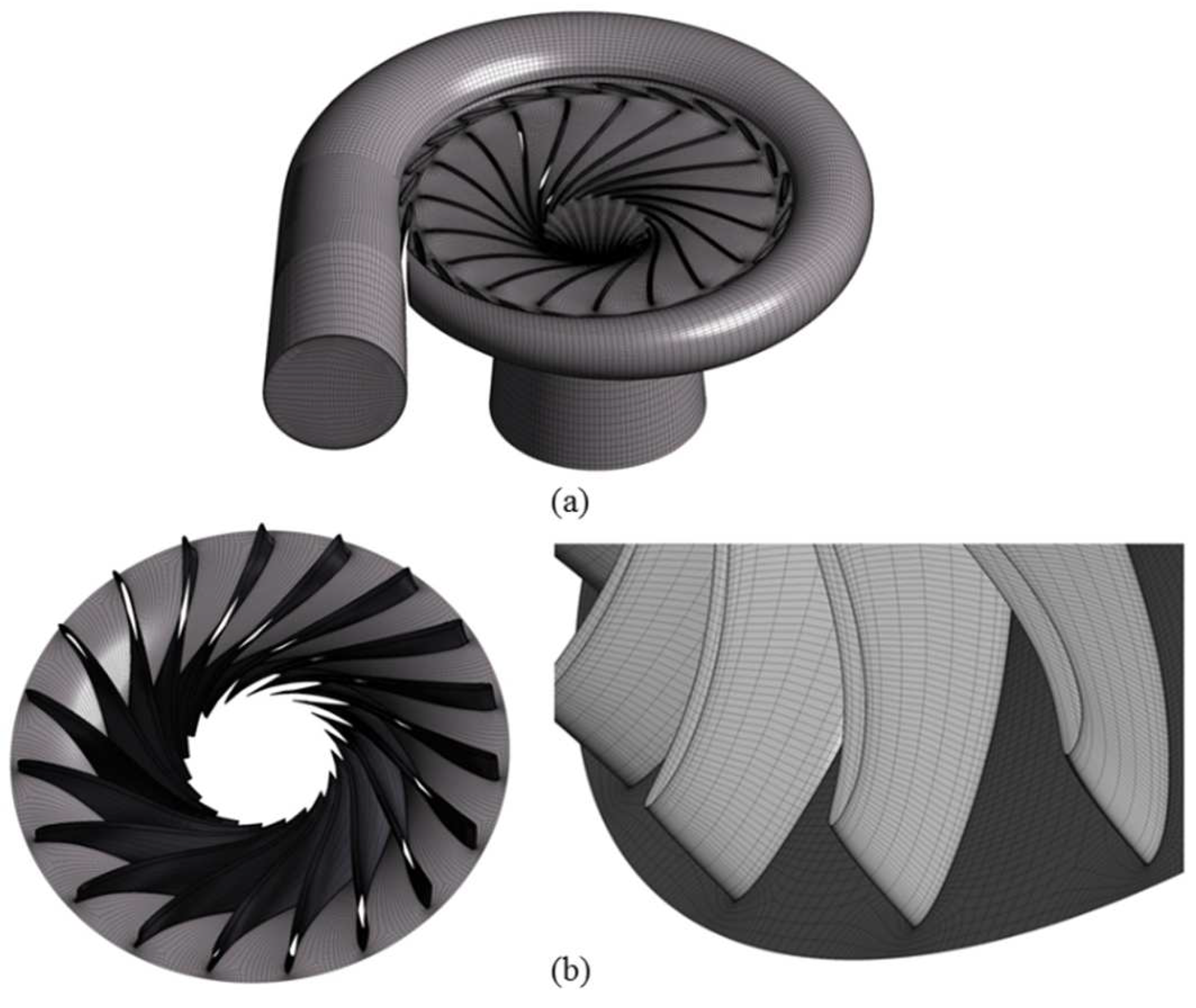
This paper generated the structural meshes of the volute, static vane, runner, and draft tube. The runner is the core component of the hydraulic turbine, and the internal flow is complicated. In order to improve the accuracy of numerical calculation, it is necessary to refine the grid in the runner region.

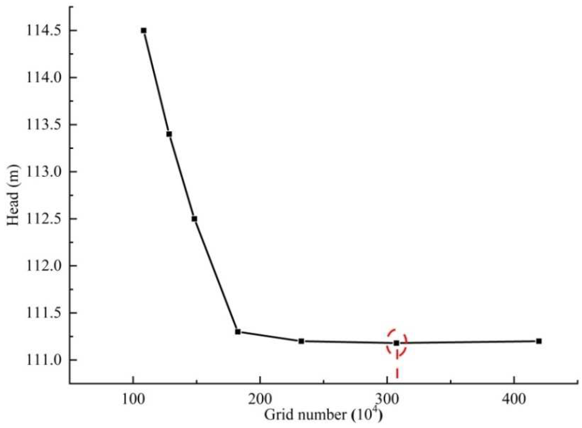
Figure 2 is a schematic diagram of the runner grid. The grid independence verification had been performed to select the appropriate grid numbers, as the calculation time and computer requirement increased with the grid number. The variation curve of the hydraulic turbine head with grid number under the optimal working condition is shown in Figure 3. When the number of grids was more than 3.03 million, the head almost kept constant. Thus, the total number of grids was 3.03 million.

2.4. The Fundamental Equations

2.4.1. Incompressible Gas Model

The water head of the hydraulic turbine represents the difference in liquid energy per unit weight between the inlet and outlet of the hydraulic turbine.

For pure liquid conditions, the head is defined as [27]:

$$H_{pure}=\frac{p_1-p_2}{\rho g}+\frac{{\overline{v}}_1^2-{\overline{v}}_2^2}{2g}+\left(z_1-z_2\right)$$

(4)

For the gas–liquid two-phase working conditions, when the gas phase is considered incompressible, the gas phase’s density is constant. It was assumed that the gas and liquid mixed uniformly. At this time, the mixing density is defined as [29]:

$${\rho }_m=\alpha {\rho }_g+\left(1-\alpha \right){\rho }_l$$

(5)

$$\alpha =Q_g/\left(Q_l+Q_g\right)$$

(6)

The head of the hydraulic turbine under gas–liquid two-phase is defined as:

$$H_{incom}=\frac{p_1-p_2}{{\rho }_{m}g}+\frac{{\overline{v}}_1^2-{\overline{v}}_2^2}{2g}+\left(z_1-z_2\right)$$

(7)

where subscripts 1 and 2 represent the inlet and outlet of the hydraulic turbine.

The hydraulic efficiency of the hydraulic turbine when the gas is considered incompressible is defined as [27]:

$${\eta }_{incom}=\frac{M\omega }{mg{H}_{incom}}$$

(8)

where m is the mass flow rate of the turbine.

2.4.2. Compressible Gas Model

The compressible gas usually absorbs heat when it expands. However, because the gas mass fraction is much lower than that of the liquid phase, the liquid phase can provide the heat absorbed by the gas during expanding process with a tiny temperature increment. Hence, the expanding process of the gas phase can be assumed to be an isothermal process. Moreover, as the quantity of heat transfer between the working fluid and the atmosphere was small and the specific heat capacity of water was large, the influence of heat transfer on the state of the working fluid can be neglected.

The energy equation of the hydraulic turbine under gas–liquid two-phase working conditions can be deduced from the fundamental thermodynamic equation for an open system [30]:

$$E_1+p_1{V}_1+Q=E_2+p_2{V}_2+W$$

(9)

$$E=U+\frac{1}{2}m{\overline{v}}^2+mgz$$

(10)

For compressible gas, its expansion process absorbs heat Q_g. Since the thermal process of gas was assumed to be an isothermal process, its internal energy remained unchanged at the inlet and outlet of the hydraulic turbine. At this time, Equations (8) and (9) can be used to obtain the energy equation of the gas phase:

$$Q_g=m{\left(\frac{1}{2}\Delta {\overline{v}}^2+g\Delta z\right)}_g+\Delta {\left(pV\right)}_g+W_g$$

(11)

Equation (10) was converted to the equation per mass:

$$q_g={\left(\frac{1}{2}\Delta {\overline{v}}^2+g\Delta z\right)}_g+\Delta {\left(pv\right)}_g+w_g$$

(12)

In an isothermal process, the heat absorbed by the gas was equal to the power:

$$q_g={\displaystyle {\int }_1^{2}p}d{v}_g$$

(13)

The technical work performed by the gas phase on the hydraulic turbine was as follows [30]:

$$w_{\mathrm{g}}=\frac{1}{2}{\left({\overline{v}}_1^2-{\overline{v}}_2^2\right)}_g+g{\left(z_1-z_2\right)}_g+{\displaystyle {\int }_2^1{v}_{g}d}p$$

(14)

$$w_{\mathrm{g}}=\frac{1}{2}{\left({\overline{v}}_1^2-{\overline{v}}_2^2\right)}_g+g{\left(z_1-z_2\right)}_g+RT\ln \frac{p_1}{p_2}$$

(15)

Then, the equivalent head was used to represent the technical work of gas:

$$H_g=\frac{RT}{g}\ln \frac{p_1}{p_2}+\frac{1}{2g}{\left({\overline{v}}_1^2-{\overline{v}}_2^2\right)}_g+{\left(z_1-z_2\right)}_g$$

(16)

For the liquid, its head can be obtained by Equation (3):

$$H_l=\frac{p_1-p_2}{{\rho }_{l}g}+\frac{1}{2g}{\left({\overline{v}}_1^2-{\overline{v}}_2^2\right)}_l+{\left(z_1-z_2\right)}_l$$

(17)

The gas mass fraction χ was defined as [29]:

$$\chi =m_g/\left(m_l+m_g\right)$$

(18)

The equivalent head of the hydraulic turbine under gas–liquid two-phase was deduced as follows:

$$H_{eq}=\chi H_g+\left(1-\chi \right)H_l$$

(19)

The hydraulic efficiency of the hydraulic turbine when the gas is considered compressible is as follows:

$${\eta }_{com}=\frac{M\omega }{mg{H}_{eq}}$$

(20)

2.4.3. Hydraulic Loss

In this paper, the hydraulic loss in the hydraulic turbine consisted of volute loss, static vane loss, runner loss, and draft tube loss. The calculation method of the hydraulic loss of the stationary parts is shown as follows:

The following equation can calculate the hydraulic loss of the stationary parts when the incompressible gas model was used [27]:

$$h_{incom}=\frac{P_{in}-P_{out}}{{\rho }_{m}g}$$

(21)

where P_in and P_out represent the inlet and outlet total pressure of the stationary parts.

The runner loss was calculated by the following equation [27]:

$$h_{r-incom}=h_r-{\eta }_{incom}\cdot H_{incom}$$

(22)

where h_r is the total pressure head at the inlet and outlet of the runner.

The relative loss is as follows:

$$c_{incom}=h_{incom}/H_{incom}$$

(23)

When the compressible gas model was used, the hydraulic loss of the stationary parts was calculated by the equations below:

$$h_{com}=\chi h_g+\left(1-\chi \right)h_l$$

(24)

$$h_l=\frac{p_{in}-p_{out}}{{\rho }_{l}g}+\frac{1}{2}{\left(v_{in}^2-v_{out}^2\right)}_l$$

(25)

$$h_g=\frac{RT}{g}\ln \frac{p_{in}}{p_{out}}+\frac{1}{2g}{\left(v_{in}^2-v_{out}^2\right)}_g$$

(26)

where $p_{in}$ and $p_{out}$ represent the inlet and outlet static pressure of the runner.

The runner loss was as follows:

$$h_{r-com}=h_r-{\eta }_{com}\cdot H_{eq}$$

(27)

The relative loss was as follows:

$$c_{com}=h_{com}/H_{eq}$$

(28)

3. Analysis of the Results

3.1. Theoretical Analysis

3.1.1. Analysis of the Head, Inlet Static Pressure and Output Power

The head, static inlet pressure, and output power of the hydraulic turbine predicted by the compressible and incompressible models under different IGVF conditions are shown in

Table 3. Head, inlet static pressure, and output power of the hydraulic turbine.

IGVF	Incompressible Model			Compressible Model
	Hincom (m)	pv-in (MPa)	Output Power (kW)	Hl (m)	Hg (m)	Heq (m)	Pv-in (MPa)	Output Power (kW)
5%	109.26	1.13	198.25	106.14	21,177	122.32	1.14	211.34
10%	109.64	1.08	186.99	101.50	21,093	135.24	1.13	209.53
15%	109.81	1.03	175.30	95.52	20,931	147.84	1.11	205.00
20%	109.93	0.97	163.60	88.76	20,722	160.60	1.09	199.04

. For the incompressible model, the head increases slowly with the IGVF, and the growth rate is about 0.2%. The gas-phase head and liquid-phase head values of the compressible results are also shown in Table 3. The liquid-phase head and gas-phase head decrease with the IGVF, but the equivalent head increases with the IGVF. At the same IGVF, the incompressible head is smaller than the equivalent head. Their difference increases with the IGVF. The static inlet pressure continuously decreases with the IGVF in the incompressible and compressible results. The static inlet pressure decreases faster in the incompressible results than in the compressible results. The output power is closely related to pressure, so the output power decreases with the IGVF. At the same IGVF, the static inlet pressure and the output power are smaller in the incompressible results than in the compressible results.

3.1.2. Analysis of External Characteristics

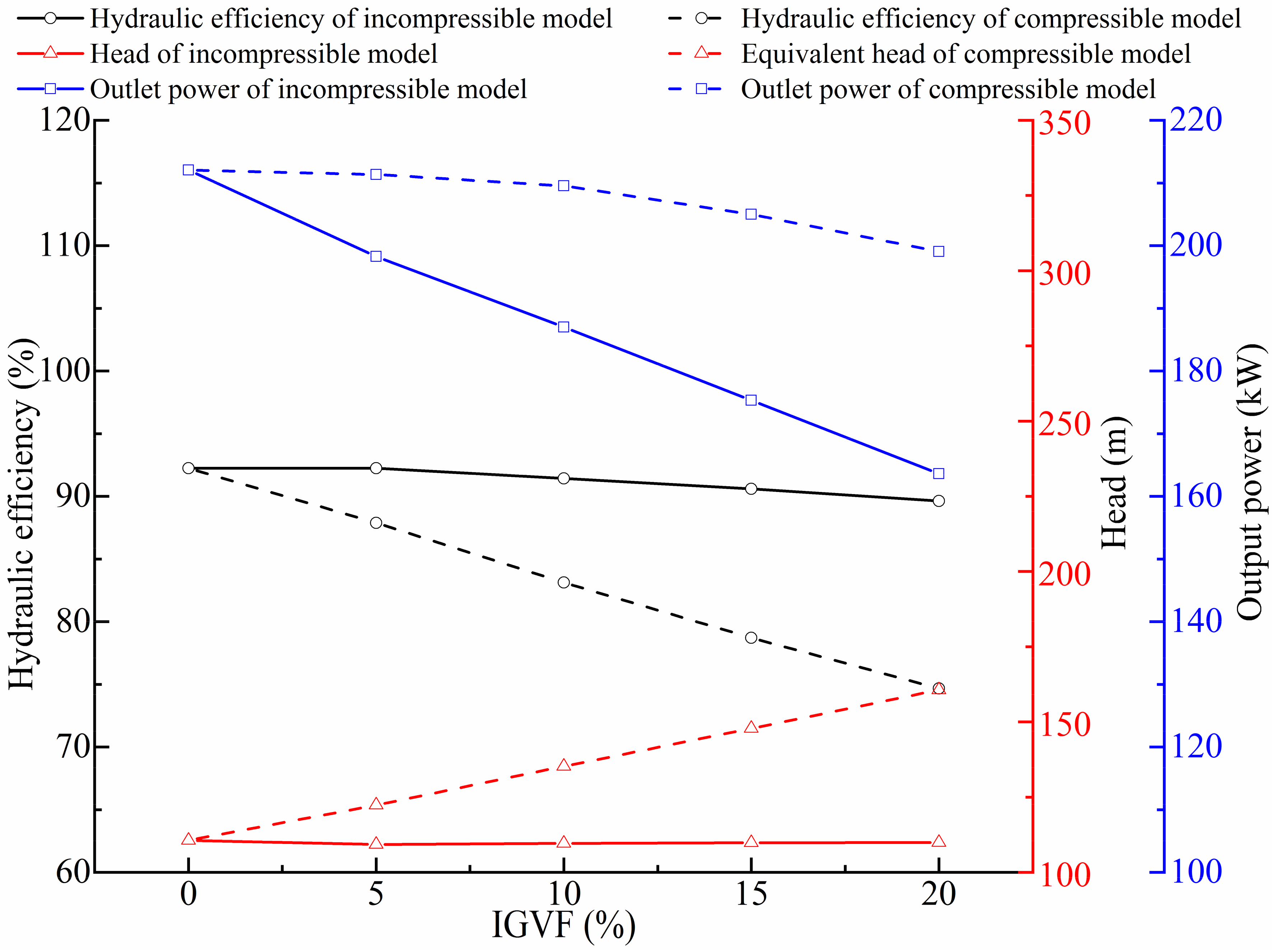
The external characteristics of the hydraulic turbine predicted by the compressible and incompressible models under different IGVF conditions are shown in Figure 4. The hydraulic efficiency and output power of the hydraulic turbine are the largest under pure liquid conditions. At this time, the hydraulic turbine has a solid ability to recover the residual pressure energy of the pressurized liquid. Two kinds of gas models predicted significant differences in the output power, head, and hydraulic efficiency. The changing trend is also different. The head for incompressible gas was calculated by Equation (6). The calculating pressure difference at the inlet and outlet continuously decreases with the increase in the IGVF. However, as the mixture density decreases with the IGVF, its head changes slightly. When the compressible gas model is used, the equivalent head consists of the gas-phase head and liquid-phase head, as shown in Equation (18). Both the liquid and gas heads decrease with the IGVF. Nevertheless, the gas head is far higher than the liquid head under the same pressure difference due to its expanding work and small density. Thus, the equivalent head increases with the IGVF and is 46% higher than the incompressible model at an IGVF of 20%.

As for output power, the output power calculated by the incompressible gas model decreases linearly with the IGVF. Because the incompressible gas generates little power as it expands, the total output power drops with the IGVF. As the effective work decreases with the reduction of mixture density, the hydraulic efficiency almost remains unchanged in the incompressible results. For the compressible model, the output power of the runner decreases slightly with the IGVF. The output power is higher than that predicted by the incompressible model, as the expanding power of the gas phase has been included. The maximum relative difference is 21.6% at the IGVF of 20%. However, because the effective work increases with the equivalent head, its hydraulic efficiency decreases rapidly and is 16.6% lower than that predicted by the incompressible model at the IGVF of 20%. Therefore, the output power of the two-phase hydraulic turbine calculated by the compressible model is higher than that predicted by the incompressible model, but the hydraulic efficiency is lower.

Xia [31] tested the performance of a pump-as-turbine with a specific speed of 40 from 0 to 20% IGVF. The variation trend of the equivalent head, output power, and hydraulic efficiency predicted by the compressible model in this paper is consistent with the test results in reference [31].

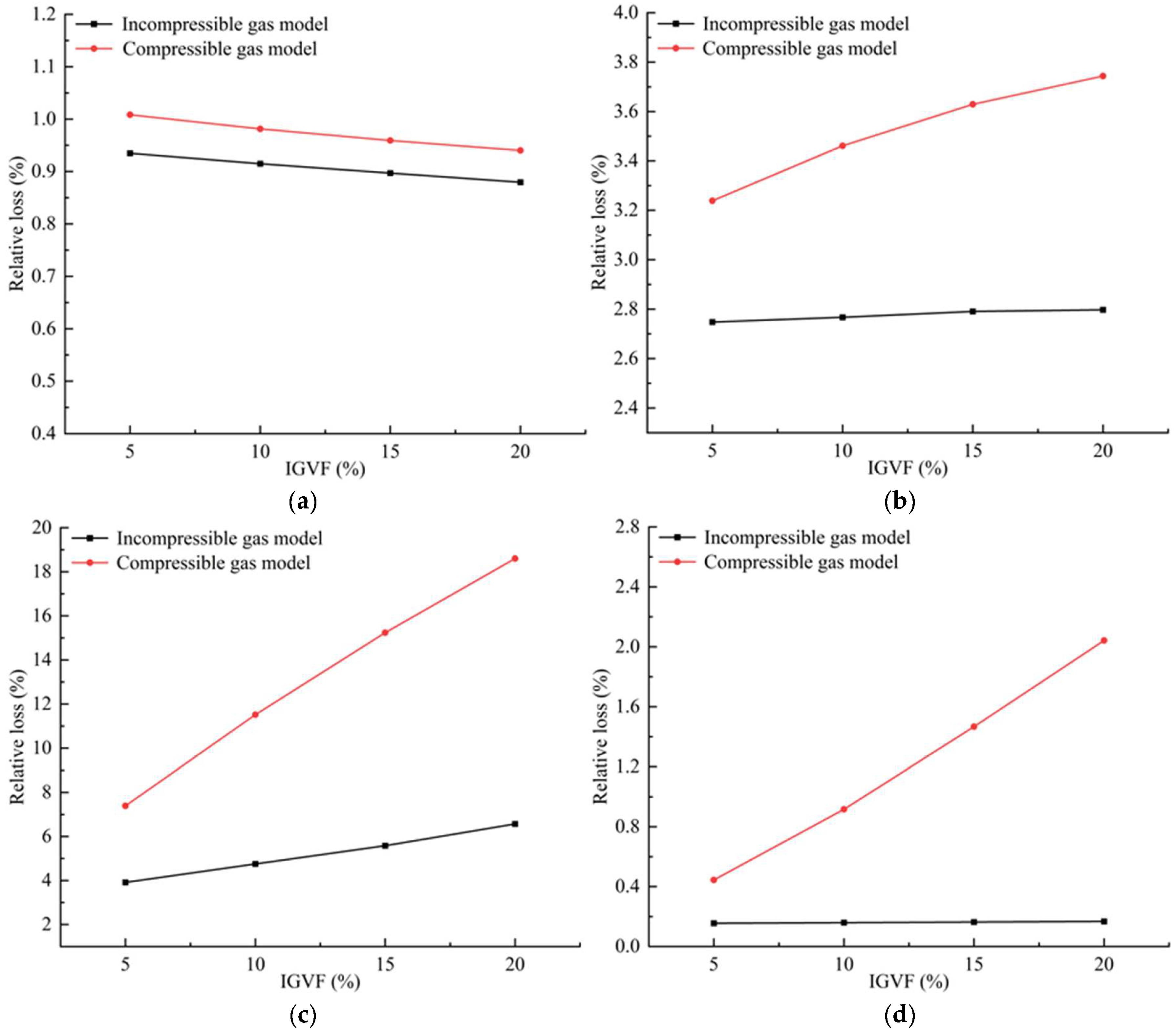
3.1.3. Loss Analysis of Each Part

The value of hydraulic loss in each part of the turbine is shown in

Table 4. Loss of the hydraulic turbine.

IGVF	Incompressible Model				Compressible Model
	hv (m)	hsv (m)	hrun (m)	hdt (m)	hv (m)	hsv (m)	hrun (m)	hdt (m)
0	1.29	3.28	3.81	0.25	1.29	3.28	3.81	0.25
5%	1.02	3.00	4.28	0.17	1.30	3.96	9.04	0.54
10%	0.99	3.03	5.21	0.17	1.33	4.68	15.58	1.24
15%	0.96	3.06	6.13	0.17	1.42	5.37	22.53	2.17
20%	0.92	3.08	7.22	0.18	1.51	6.01	29.88	3.28

. It can be seen from the table that the loss predicted by the compressible gas model is greater than the incompressible gas model under different IGVF conditions. As the IGVF increases, the hydraulic loss in the volute decreases in the incompressible results while it increases in the compressible results. This is because the water mass flow rate decreases with the IGVF, the water flow loss decreases in the incompressible results, and the gas loss increases in the compressible results. Both the static vane’s loss and the runner’s loss increase gradually with the IGVF in the compressible and incompressible results. Notably, the difference in the runner’s loss predicted by the two gas models increases significantly with the IGVF.

Figure 5 shows the variation curves of the relative loss in each part of the turbine predicted by two gas models. At the same IGVF, the relative loss predicted by the compressible gas model is more than the incompressible gas model. The main reason is the loss of expansion work and the influence of gas compressibility on the liquid flow field.

In the volute, the relative loss decreases with the IGVF. As the homogeneous two-phase flow flows into the volute, the GVF distribution is relatively uniform, and the flow pattern is good. For the incompressible model, the hydraulic loss in the volute is mainly the flow friction loss. With the increase in the GVF, the density and viscosity of the fluid decrease, so the hydraulic loss decreases. For the compressible model, the expansion loss and total hydraulic loss increase with the IGVF. However, as the equivalent head for the compressible model increases a lot, the relative loss also decreases. The relative loss in the static vane of the compressible results increases remarkably with the IGVF and accounts for 3.8% maximally. The primary loss in the turbine happens at the runner. The maximum relative loss reaches 19% in the compressible results at the IGVF of 20%. When the gas compressibility is considered, the gas expansion in the runner leads to the increase in two-phase velocity and the TKE. Therefore, the runner loss in the compressible results increases sharply with the IGVF. In the draft tube, the relative loss of the incompressible results is only 0.2%, while the relative loss of the compressible results increases to 2%, which is higher than that in the volute. The main reason is that the two-phase velocity in the draft tube predicted by the compressible model is high.

3.2. Analysis of the Flow Field

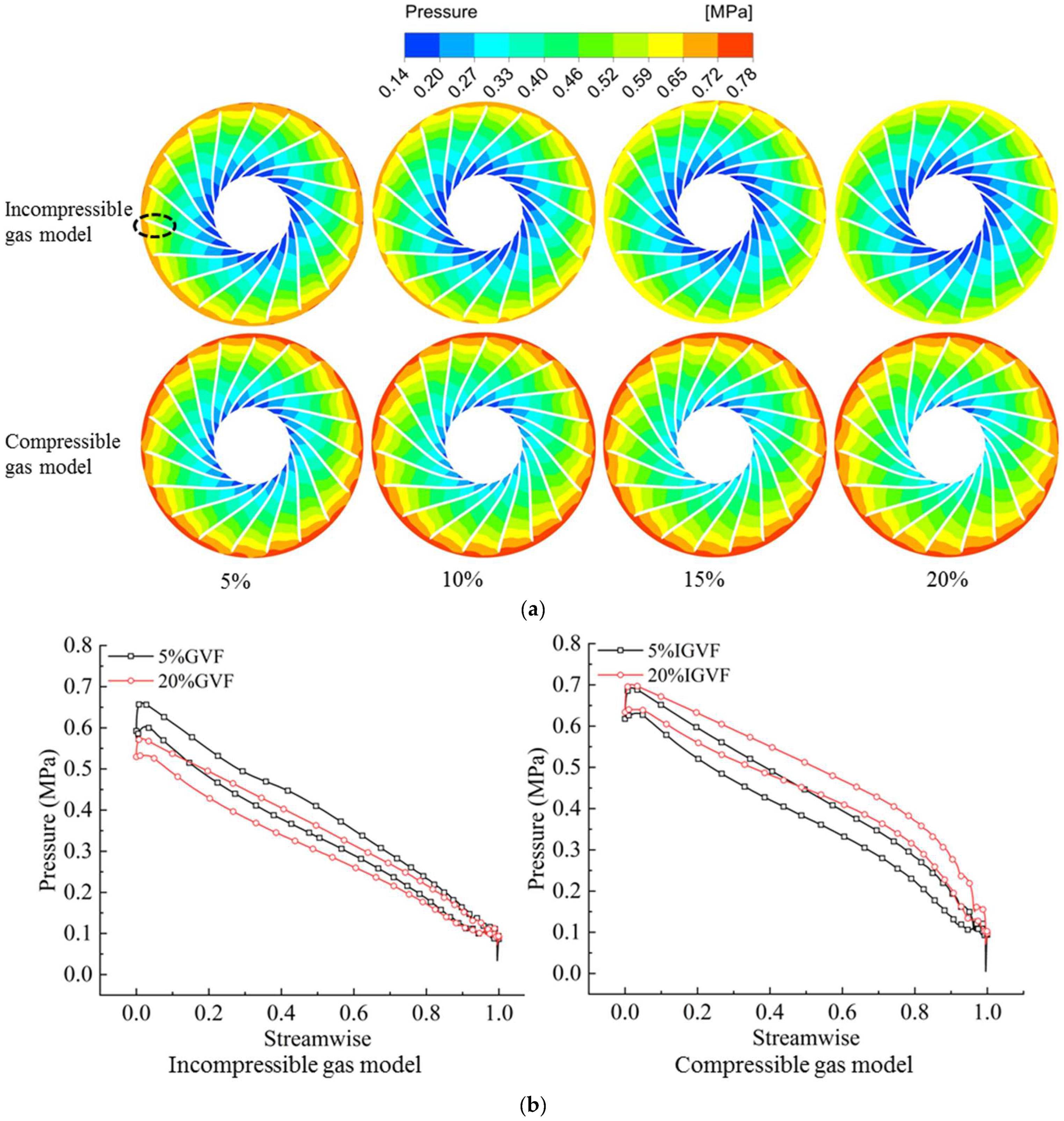
3.2.1. Static Pressure Distribution

Figure 6 shows the static pressure distribution in the runner under the variable IGVF when the incompressible and compressible models were used. In Figure 6a, the pressure gradient exists in the runner. The low-pressure zone near the outlet of the runner in the incompressible results is larger than in the compressible results under all IGVF conditions. Moreover, the low-pressure zone area in the incompressible results increases with the IGVF. However, it decreases with the IGVF in the compressible results. Figure 6b shows the pressure curve on the surface of one blade at 5% and 20% IGVF, respectively. The selected blade is marked with a black circle in Figure 6a. Firstly, in the incompressible results, the inlet pressure of the blade decreases with IGVF. Secondly, the area of the pressure line at 20% IGVF is lower than that at 5% IGVF. It means that the output power of the blade decreases with the IGVF. Furthermore, as the simulation adopts the boundary conditions of the inlet mass flow rate and the outlet pressure, the inlet pressure of the blade decreases due to the lower output power. Hence, the low-pressure zone increases with the IGVF.

In contrast, in the compressible results, the low-pressure zone decreases with the IGVF. In Figure 6b, the pressure curve at 20% IGVF is higher than that at 5% IGVF. The reason is that the gas expands in the blade passage with the pressure reduction. At the same time, as the gas volume increases, the reduction rate of the pressure decrease.

Moreover, the area of the pressure curve at 20% IGVF is slightly lower than that at 5% IGVF. It means that the output power of the blade decreases little at high IGVF, which agrees with the output powers trend in Figure 4. Therefore, the inlet pressure of the blade almost keeps unchanged with the IGVF. Furthermore, the low-pressure zone in the compressible results is smaller than in the incompressible results under all IGVF conditions.

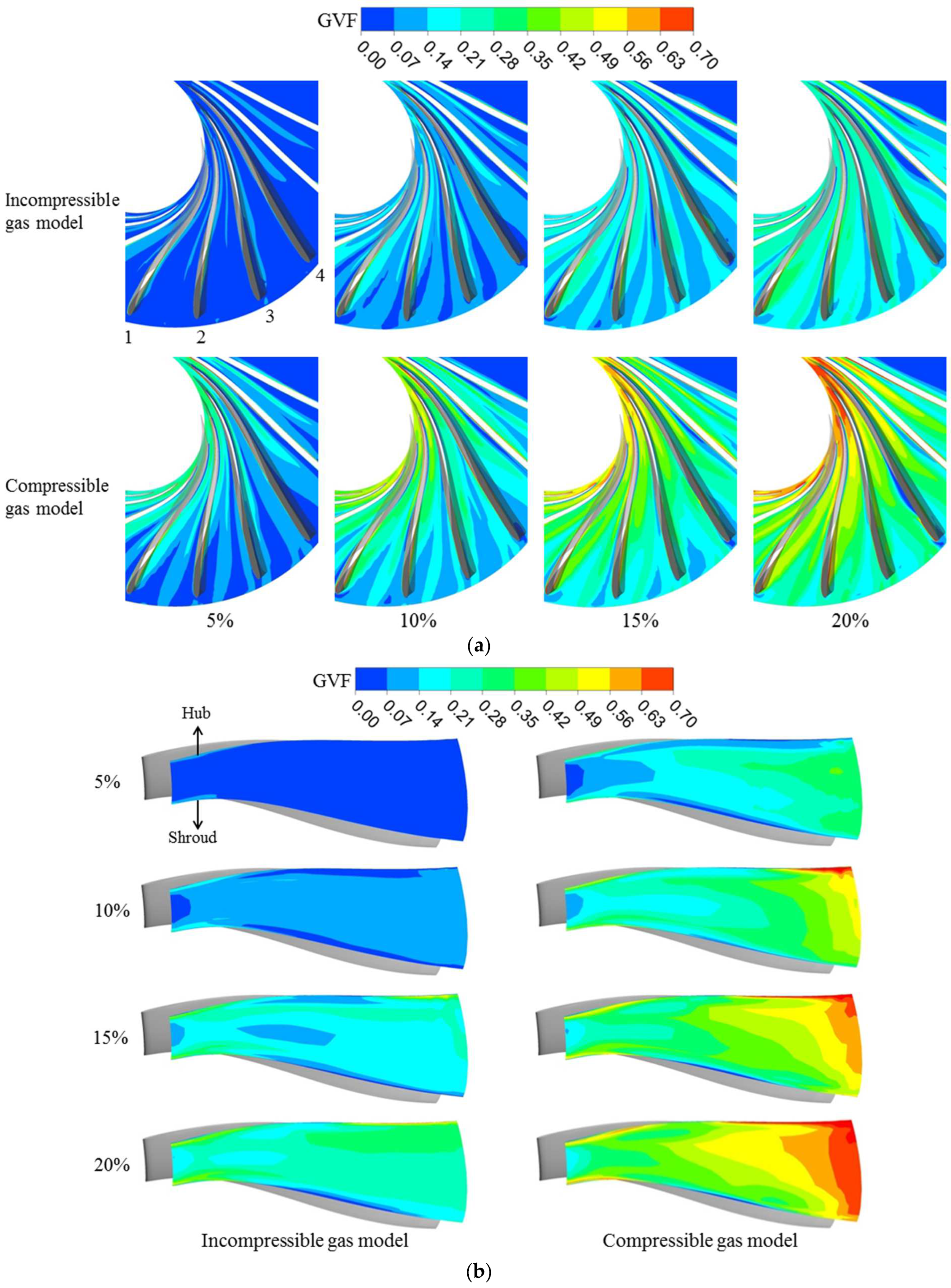
3.2.2. GVF Distribution

The GVF distribution cloud contours in the turbine under the inlet GVF of 5%, 10%, 15%, and 20% are shown in Figure 7.

The GVF distribution at a 0.5 span of the runner is shown in Figure 7a. For the incompressible gas model, the gas density does not change in the turbine. The GVF distribution varies slightly along the runner passage. At the low IGVF, the gas mainly accumulates on the working surface of the runner blade. As the IGVF increases, the gas diffuses from the blade’s working surface to its suction surface. The gas expansion is considered in the compressible gas model, so the gas accumulation predicted by the compressible model in the runner flow passage is more evident than in the incompressible results. At the low IGVF, the GVF on the blade’s working surface is higher than that predicted by the incompressible model. With the increase in the IGVF, more gas accumulates at the outlet of the runner.

Figure 7b shows the GVF distribution on the working surface of blade 3. The GVF distribution is relatively uniform in incompressible results and changes little along the flow passage. In contrast, the GVF distribution of compressible results increases significantly along the flow passage. The high GVF areas exist near the hub at the exit of the blade passage. As the IGVF increases, the high GVF areas become larger. That is because the pressure near the hub in the blade passage is lower than that near the shroud. The gas accumulates in the low-pressure area due to the adverse pressure gradient.

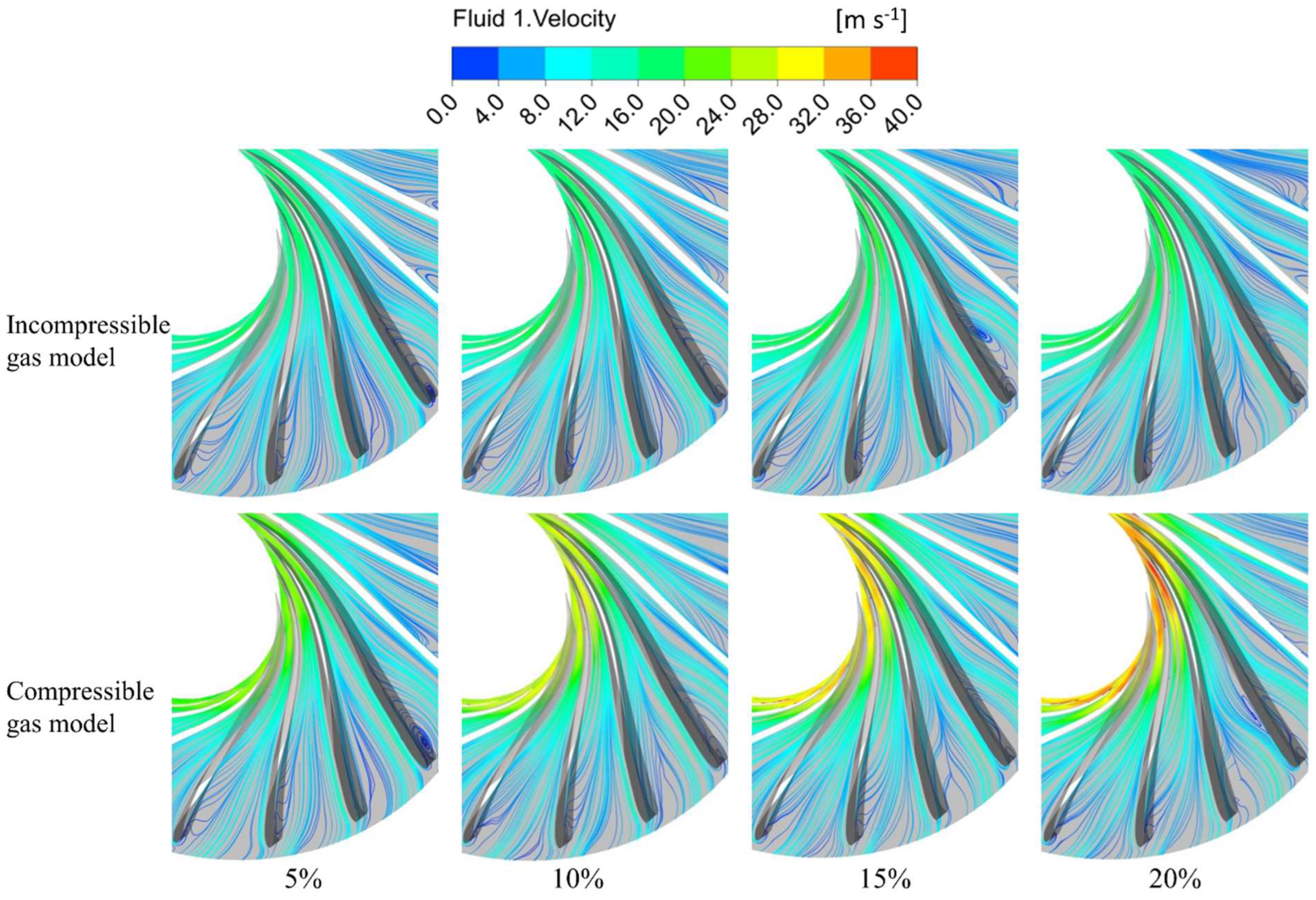
3.2.3. Velocity and Streamlines

Figure 8 shows the liquid phase velocity and streamlines in the runner at variable IGVF when the incompressible and compressible models were used. It can be seen that the liquid accelerates in the runner flow passage, and the flow velocity on the suction surface is larger than on the working surface of the blade. The reason is that the water impacts the working surface of the blade, causing phenomena, such as flow separation, and vortices on the working surface. As a result, most fluid flows along the suction surface, resulting in a higher flow velocity.

The velocity at the runner outlet in the incompressible results is less than that in the compressible results when the IGVF is the same. With the increase in the IGVF, the velocity at the runner outlet does not change significantly in the incompressible results. In contrast, the velocity at the runner outlet in the compressible results increases by 39.5% when the IGVF increases from 5% to 20%. This phenomenon is because a large amount of gas accumulates at the runner outlet in the compressible results. The higher the IGVF, the more intense the gas accumulation, as shown in Figure 7. The accumulation of gas reduces the flow area for the liquid in the blade passage, which results in high-velocity liquid.

3.2.4. Turbulence Kinetic Energy Distribution

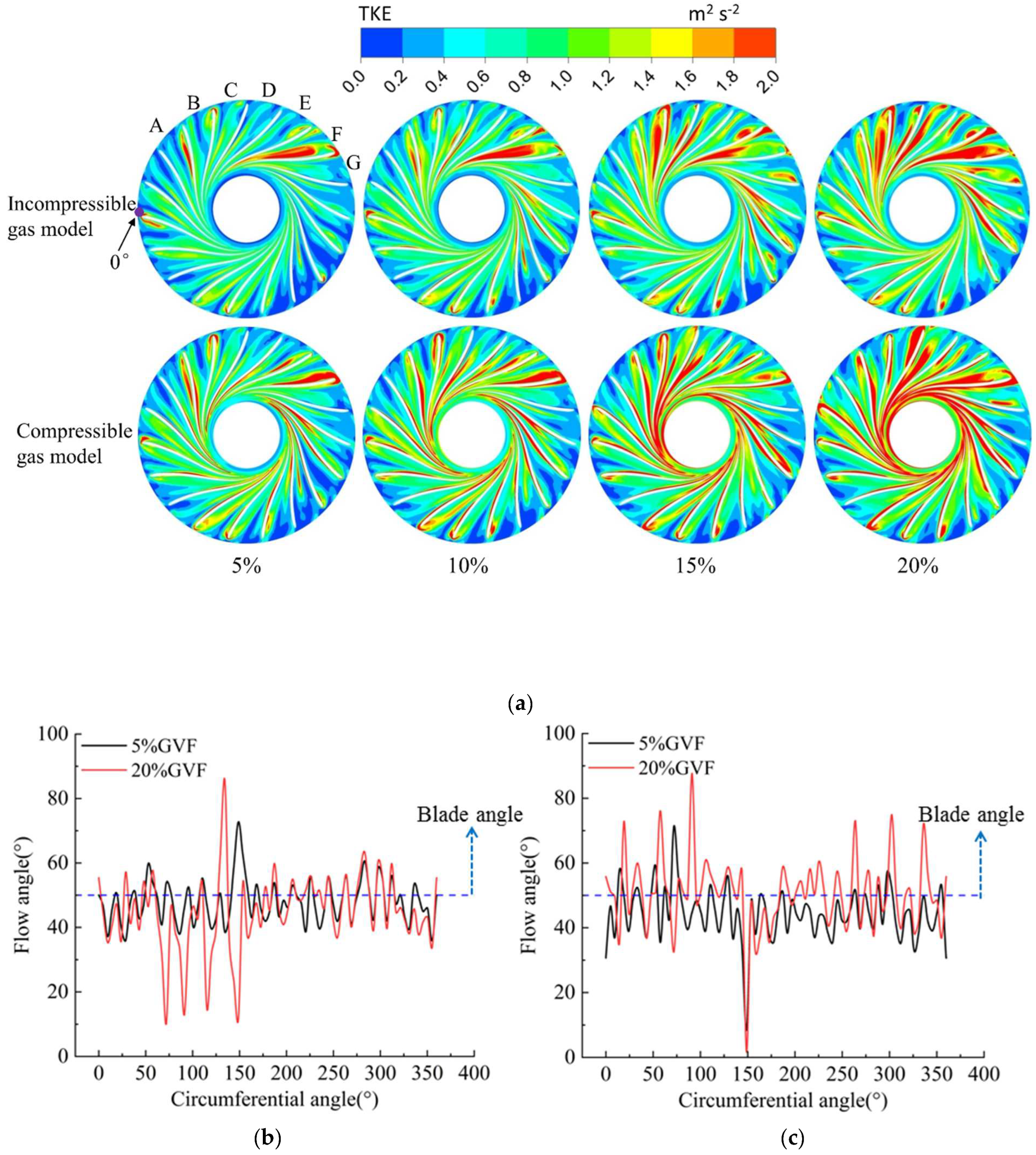
Figure 9a shows the Turbulent Kinetic Energy (TKE) distribution in the runner predicted by different gas models from 5% to 20% of IGVF. The TKE is related to the velocity fluctuations, reflecting the energy loss characteristics and the degree of turbulence.

In Figure 9a, when the IGVF is 5%, high TKE distribution areas appear in blade passage F near the volute tongue in compressible and incompressible results. The flow field in the blade passage near the volute tongue is quite chaotic. Inlet impact and flow separation happen in the blade passage, resulting in a considerable TKE in the channel.

With the increase in the IGVF, the high TKE distribution areas gradually appear in the nearby upstream blade passage B to F. In order to further analyze the reason for this phenomenon, the liquid flow angle distributions in incompressible results under the 5% and 20% IGVF are shown in Figure 9b. The purple point in Figure 9a is the position of the 0° circumferential angle. The liquid flow angle refers to the angle between the relative velocity of the flow and the circumferential velocity at the inlet of the runner. The liquid flow angle at 5% IGVF reaches its peak value when the circumferential angle is 148°, corresponding to the blade passage F. The excessive liquid flow angle causes severe inlet impact, which results in a high TKE distribution. With the increase in the IGVF, the inlet liquid flow angle of the runner varies since the inlet liquid velocity changes with the IGVF. At 20% of IGVF, the flow near the volute tongue deteriorates. Large negative attack angles happen when the circumferential angle increases from 72° to 148°, which induces the high TKE distribution areas in blade passages B, C, D and F. At the same time, the peak value exists at the circumferential angle of 134°, corresponding to the high TKE area at the blade passage E and the suction surface of the blade.

For compressible results, the distribution area of high TKE appears on the suction surface of the blade at all IGVF conditions, as shown in Figure 9a. The reason is that the gas accumulates on the working surface of the blade, and the liquid phase is squeezed onto the suction surface, as shown in Figure 7, resulting in a large flow velocity near the suction surface. The high TKE distribution area near the runner outlet changes obviously with the IGVF. The higher the IGVF, the larger the TKE distribution area at the runner outlet. This is because more gas expands in the blade passage and takes up more space as the IGVF increases. Thus, the liquid velocity and the TKE increase quickly with the IGVF. The high TKE areas in the compressible results are also related to the liquid flow angle, as shown in Figure 9c. When the IGVF is 5%, the negative attack angles exist at the blade passages B and F. When the IGVF is 20%, compared to the incompressible results, more impact loss happens at the inlet of the runner and causes a larger high TKE area, especially when the circumferential angle changes from 260° to 360°.

The above analysis shows that the increase in the IGVF causes the variation of the inlet liquid flow angle, which leads to the impact loss at the inlet of the blade passages and the high TKE areas. For the compressible results, the impact loss at the inlet of the blade passage and the flow velocity in the blade passage are higher than that in the incompressible results, resulting in larger high TKE areas and hydraulic loss in the runner.

4. Conclusions

The paper simulated the hydraulic turbine under different IGVF with the incompressible and compressible models, respectively. The equivalent head, hydraulic efficiency, and flow loss considering the expanding work of compressible gas were deduced based on the energy conservation equations. Then, the incompressible and compressible results are compared and analyzed. The conclusions are summarized as follows.

(1) Due to the expanding work of compressible gas, the equivalent head, output power and the relative hydraulic loss predicted by the compressible gas model are higher than the incompressible model, but the hydraulic efficiency is lower. Furthermore, the equivalent head predicted by the compressible gas model increases rapidly with the IGVF, but the incompressible gas model’s results remain unchanged. The trend of the equivalent head in the compressible results is consistent with the test results.

(2) The pressure and GVF distributions predicted by the different gas models are different. The low-pressure zone in the blade passage in the incompressible results is larger than the compressible results under all IGVF conditions. Moreover, the area of the low-pressure zone in the incompressible results increases with the IGVF. However, it decreases with the IGVF in the compressible results.

The gas accumulation on the blade’s working surface in the compressible results is more severe than in the incompressible results. As the IGVF increases, the gas gradually diffuses from the blade’s working surface to its suction surface. The gas–liquid separation happens at the runner outlet in the compressible results due to the gas expansion.

(3) The runner’s inlet gas distribution affects the liquid flow angle, causing the inlet shock and high TKE areas, especially in the blade passage near the volute tongue. The high TKE area in the compressible results is larger than the incompressible results because inlet impact loss and the liquid velocity in the blade passage are higher than that in the incompressible results.

(4) The compressible gas model should be used in the numerical simulations of this paper for the large performance difference predicted by different gas models. When the IGVF is lower than 5%, the difference may be negligible under a certain IGVF. Future work can be conducted to find the IGVF under which the incompressible gas model can be used reasonably.

References

- Yang, J.H.; Zhang, X.N.; Wang, X.H.; Sun, Q.Z.; Zhang, J.H. Overview of research on energy recovery hydraulic turbine. Fluid Mach. 2011, 39, 29–33. [Google Scholar]
- Williams, A.A. The turbine performance of centrifugal pumps: A comparison of prediction methods. Proc. Inst. Mech. Eng. Part A J. Power Energy 1994, 208, 59–66. [Google Scholar] [CrossRef]
- Kramer, M.; Terheiden, K.; Wieprecht, S. Pumps as turbines for efficient energy recovery in water supply networks. Renew. Energy 2018, 122, 17–25. [Google Scholar] [CrossRef]
- Zhang, F.; Zhu, L.F.; Chen, K.; Yan, W.C.; Appiah, D.; Hu, B. Numerical simulation of gas–liquid two-phase flow characteristics of centrifugal pump based on the CFD-PBM. Mathematics 2020, 8, 769. [Google Scholar] [CrossRef]
- He, L.; Zhang, J.Y.; Zhang, Z.M.; Meng, L.; Zhu, H.W.; Li, T.Y. Numerical simulation of the influence of design parameters on gas–liquid transport characteristics of centrifugal pump. IOP Conf. Ser. Earth Environ. Sci. 2021, 627, 012005. [Google Scholar] [CrossRef]
- Singh, P.; Nestmann, F. Internal hydraulic analysis of impeller rounding in centrifugal pumps as turbines. Exp. Therm. Fluid Sci. 2011, 35, 121–134. [Google Scholar] [CrossRef]
- Zhu, J.J.; Zhang, H.Q. Numerical study on electrical-submersible-pump two-phase performance and bubble-size modeling. SPE Prod. Oper. 2017, 32, 267–278. [Google Scholar] [CrossRef]
- Sun, L.G.; Guo, P.C.; Luo, X.Q. Numerical investigation on inter-blade cavitation vortex in a Francis turbine. Renew. Energy 2020, 158, 64–74. [Google Scholar] [CrossRef]
- Sun, L.G.; Guo, P.C.; Luo, X.Q. Numerical investigation of inter-blade cavitation vortex for a Francis turbine at part load conditions. IET Renew. Power Gener. 2021, 15, 1163–1177. [Google Scholar] [CrossRef]
- Huang, S.; Su, X.H.; Guo, J.; Yue, L. Unsteady numerical simulation for gas–liquid two-phase flow in self-priming process of centrifugal pump. Energy Convers. Manag. 2014, 85, 694–700. [Google Scholar] [CrossRef]
- Caridad, J.; Kenyery, F. CFD analysis of electric submersible pumps (ESP) handling two-phase mixtures. J. Energy Resour. Technol. 2004, 126, 99–104. [Google Scholar] [CrossRef]
- Suh, J.W.; Kim, J.W.; Choi, Y.S.; Kim, J.H.; Joo, W.G.; Lee, K.Y. Development of numerical Eulerian-Eulerian models for simulating multiphase pumps. J. Pet. Sci. Eng. 2018, 162, 588–601. [Google Scholar] [CrossRef]
- Zhang, W.W.; Yu, Z.Y.; Zahid, M.N.; Li, Y.J. Study of the gas distribution in a multiphase rotodynamic pump based on interphase force analysis. Energies 2018, 11, 1069. [Google Scholar] [CrossRef]
- Zhang, W.W.; Zhu, B.S.; Yu, Z.Y. Characteristics of bubble motion and distribution in a multiphase rotodynamic pump. J. Pet. Sci. Eng. 2020, 193, 107435. [Google Scholar] [CrossRef]
- Ge, Z.G.; He, D.H.; Huang, R.; Zuo, J.L.; Luo, X.Q. Application of CFD-PBM coupling model for analysis of gas–liquid distribution characteristics in centrifugal pump. J. Pet. Sci. Eng. 2020, 194, 107518. [Google Scholar] [CrossRef]
- Sun, S.H.; Pang, Y.; Guo, P.C.; Zheng, X.B.; Yan, J.G.; He, D.H.; Luo, X.Q. Numerical simulation of two-phase flow in an energy recovery micro-hydraulic turbine based on Francis hydraulic model. IOP Conf. Ser. Earth Environ. Sci. 2019, 240, 042006. [Google Scholar] [CrossRef]
- Chen, T.J.; Sun, S.H.; Pang, Y.; Guo, P.C. Numerical analysis of two-phase flow in a micro-hydraulic turbine. Int. J. Fluid Mach. Syst. 2019, 12, 430–438. [Google Scholar] [CrossRef]
- Kim, J.H.; Jung, U.H.; Kim, S. Uncertainty analysis of flow rate measurement for multiphase flow using CFD. Acta Mech. Sin. 2015, 31, 698–707. [Google Scholar] [CrossRef]
- Yan, S.N.; Sun, S.H.; Luo, X.Q.; Chen, S.L.; Feng, J.J. Numerical investigation on bubble distribution of a multistage centrifugal pump based on a population balance model. Energies 2020, 13, 908. [Google Scholar] [CrossRef]
- Poullikkas, A. Effects of two-phase liquid-gas flow on the performance of nuclear reactor cooling pumps. Energy 2003, 42, 3–10. [Google Scholar] [CrossRef]
- Si, Q.R.; Gérard, B.; Liao, M.Q.; Zhang, H.Y.; Cui, Q.L.; Yuan, S.Q. A comparative study on centrifugal pump designs and two-phase flow characteristic under inlet gas entrainment conditions. Energies 2020, 13, 65. [Google Scholar] [CrossRef] [Green Version]
- Shi, F.X.; Yang, J.H.; Wang, X.H. Unsteady analysis of effect on hydraulic turbine under variable gas content. J. Aerosp. Power 2017, 32, 2265–2272. [Google Scholar]
- Shi, F.X.; Yang, J.H.; Wang, X.H. Analysis on characteristics of gas–liquid two-phase hydraulic turbine under variable working conditions. Fluid Mach. 2018, 46, 40–45. [Google Scholar]
- Shi, F.X.; Yang, J.H.; Miao, S.C.; Wang, X.H. Investigation on the power loss and radial force characteristics of pump as turbine under gas–liquid two-phase condition. Adv. Mech. Eng. 2019, 11, 1–10. [Google Scholar]
- Shi, G.T.; Liu, Y.; Luo, K. Analysis of gas–liquid two-phase flow field in hydraulic turbine considering gas compressibility. J. Eng. Therm. Energy Power 2018, 33, 40–46. (In Chinese) [Google Scholar]
- Shi, G.T.; Peng, J.W. Analysis of hydraulic loss in hydraulic turbine under gas–liquid two-phase condition. Pump Technol. 2018, 49, 107–112, 268. (In Chinese) [Google Scholar]
- Nechleba, M. Hydraulic Turbines-Their Design and Equipment; Constable & Co Ltd.: London, UK, 1957. [Google Scholar]
- Ansys Inc. ANSYS CFX-Solver Theory Guide; Ansys Inc.: Canonsburg, PA, USA, 2019. [Google Scholar]
- Brennen, C.E. Fundamentals of Multiphase Flows; Cambridge University Press: Cambridge, UK, 2005. [Google Scholar]
- Burghardt, M.D.; Harbach, J.A. Engineering Thermodynamics, 4th ed.; Harper Collins College Publishers: New York, NY, USA, 1993. [Google Scholar]
- Xia, S.Q. Study on the Basic Equation and Conversion Relation Curves of Hydraulic Turbine with Gas-Liquid Two Phase Medium; Lanzhou University of Technology: Lanzhou, China, 2013. (In Chinese) [Google Scholar]