Health Monitoring of Pressure Regulating Stations in Gas Distribution Networks Using Mathematical Models

Abstract

Many cities have extensive distribution networks that supply natural or town gas to domestic, industrial, and power plant consumers. A typical network may have hundreds of pressure regulating stations that are of different types and capacities, but most legacy networks are sparsely instrumented. The reliability of these stations is the first priority for ensuring uninterrupted gas supplies; hence, condition monitoring and prescriptive maintenance are critical. In this study, mathematical models were developed for two types of commonly used regulators: spring-loaded and lever-type regulators. We also considered three faults that are typically of interest: filter choking, valve seat damage, and diaphragm deterioration. The proposed methodologies used the available measured data and mathematical models to diagnose faults, track prognoses, and estimate the remaining useful life of the regulators. The applicability of our proposed methodologies was demonstrated using real data from an existing distribution network. To facilitate industrial use, the methodologies were packaged into a user-friendly dashboard that could act as an interface with the operational database and display the health status of the regulators.

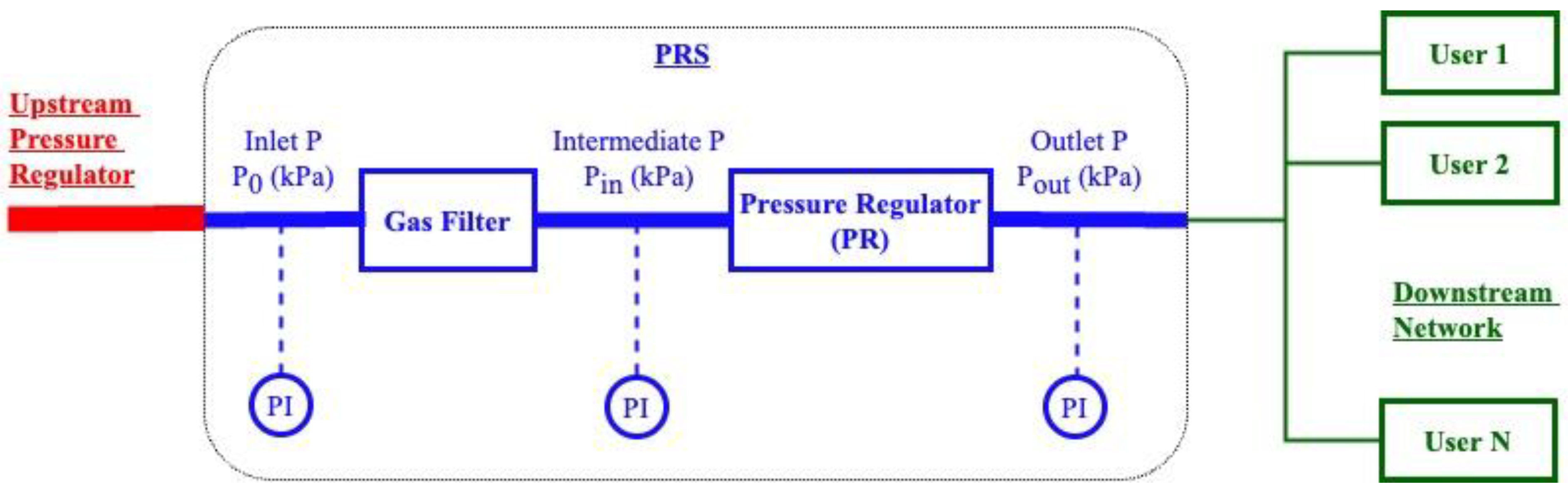
1. Introduction

Huge networks of pipelines, called gas distribution networks (GDNs), that have hundreds of pressure regulating stations (PRSs) are used to supply natural or town gas to industrial, commercial, and residential users. A PRS steps down its inlet gas pressure and maintains its outlet gas pressure at a desired set point, regardless of the gas demand profile. Gas distribution companies carefully monitor PRSs for both gradual condition deterioration and abrupt faults. Any problems need to be identified and rectified quickly to avoid disruptions in gas supplies to consumers as the companies may face regulatory penalties for such disruptions and/or lose consumer confidence.

A PRS has two components: a gas filter and a pressure regulator (PR) (Figure 1). PRs can be divided into two categories: spring-loaded (or self-operated or direct acting) regulators and pilot regulators. A spring-loaded PR has three parts: a restriction device (orifice), a sensing device (diaphragm), and a loading device (spring). Pilot regulators are used for better control accuracy and the spring is replaced by a more constant diaphragm loading force (e.g., gas pressure). PRSs can have single, dual or multiple stages. Multiple stages offer steadier outlet pressures.

Most studies on PRSs have focused on modeling and stability issues. In the literature, three approaches have been used to model PRs: an equation-based first principles approach [1], a data-driven approach [2], and a bond graph simulation technique [3,4]. Nabi et al. [5] developed a mathematical model for dome-loaded PRs and explored the impact of several geometrical and operational parameters on their performance. Rami et al. [6] developed mathematical models for direct acting and pilot-controlled PRs and identified the parameters that were responsible for their instability. Zafer and Luecke [7] developed a dynamic mathematical model for a spring-loaded PRs, studied the possible causes of vibrations, and suggested design modifications. Wang et al. [8] developed a dynamic model and self-tuning method for pneumatic pressure regulating stations. Several other studies [9,10,11,12] have also addressed the dynamic modeling of PRs. Recently, several studies have focused on the development of data-driven methodologies for the monitoring and fault diagnosis of gas pressure regulators [13,14,15,16,17].

Leo et al. [1] simulated a GDN to study the health monitoring of PRSs. They studied four faults: spring decay, filter choking, diaphragm malfunction, and valve seat damage. Three scenarios were studied for filter choking and spring decay: P_out (outlet pressure) and flow data at the same sampling rates, P_in (intermediate pressure) and P_out data at the same sampling rates, and P_out and cumulative flow data at different sampling rates. To monitor the valve seat condition, the weekly average of the daily maximum P_out values was used, whereas the hourly mean of P_out was used to monitor the diaphragm condition.

Based on our industry interactions, PRSs can develop five types of health degradations and/or faults: the overloading of the downstream network, spring decay, filter choking, valve seat damage, and diaphragm malfunctions. Spring decay, filter choking, and the overloading of downstream networks cause downstream under-pressure, whereas valve seat damage results in over-pressure. PRSs can experience slow (e.g., spring decay and diaphragm malfunctions) and/or fast (e.g., filter choking and valve seat damage) degradation. Over time, the springs lose their stiffness and the diaphragms lose their flexibility of movement due to fatigue (cyclic stress). The filters that are placed upstream of PRs to remove particles can choke with time. In the case of valve seat damage, the flows through regulators can stop completely.

Over the years, the maintenance paradigm for physical systems has improved from reactive maintenance (fixing faults after they occur) to preventive (performing routine repairs), then predictive (predicting failures and then repairing them), and finally prescriptive maintenance (predicting failures and recommending action). PRSs are usually monitored for gradual health deterioration and abrupt faults. Hence, real-time monitoring and automated prescriptive maintenance are crucial for the smooth operation of GDNs. As seen in Figure 1, pressure can be measured at three locations: upstream of the gas filter, between the filter and regulator, and downstream of the PR. Most existing PRSs are sparsely instrumented. The intermediate pressure (P_in in Figure 1) is not measured in many PRSs. Most often, the data that are collected from PRSs are not automatically transferred to the respective control rooms. Depending on the availability of pressure and flow data, either model-based or data-based methods can be applied for PRS health monitoring.

Currently, gas distribution companies perform routine preventive maintenance on PRSs. Maintenance teams visit PRSs every six months for inspection and repair. In the worst-case scenario, the sudden failure of a PRS can lead to unexpected disturbances in the gas supply. This study developed methodologies for the prescriptive maintenance of filters, valve seats, and diaphragms. Spring decay was not considered as it occurs rarely and very slowly (the average lifetime of springs is more than 10 years). Firstly, first principles models were developed for spring-loaded and lever-type PRs. Note that lever-type PRs also use springs. Data that were provided by the PRS vendors were used to calibrate the developed mathematical models. The first principles health monitoring models could be computationally expensive. Hence, as an alternative, the first principles models were simplified to estimate flows more quickly with comparable accuracy. Most gas distribution companies only measure flows at the end-use points (households, industry, power plants, etc.) and the huge number of end users makes it difficult to estimate the total gas consumption within a geographical area. The developed first principles models could provide estimates of the gas flows through PRSs. Gas companies could use this information for advanced planning to avoid the overloading of downstream networks.

The main contributions of the present study are summarized below:

• Mathematical models for two different regulator types: spring-loaded and level-type regulators (the spring-loaded regulators had a significantly different valve seat geometry than those that were studied by Leo et al. [1]);
• Precise PR dimensions and calibration data that were obtained from the PRS vendors to determine the mathematical model parameters (in contrast, Leo et al. [1] assumed some parameters);
• In contrast to Leo et al. [1], this work used real data from a large existing GDN comprising both industrial and residential end-users (the GDN did not measure the flows through the PRs and rarely measured P_in);
• Significantly modified and advanced monitoring algorithms to address the following challenges for more robust and improved inferences: (a) higher noise levels in industrial data compared to the white noise that has been added to synthetic data, (b) the absence of some data from the GDN, and (c) pressure sensor errors in real data;
• A filter monitoring methodology that used P_in (or P_o when P_in was not available) and P_out, whereas valve seat and diaphragm monitoring only required P_out (these advances are detailed in the Fault Monitoring Methodologies section).

In the prescriptive maintenance of PRSs, the estimation of remaining useful life (RUL) is crucial for uninterrupted gas supplies. The proposed health monitoring methodologies could predict RUL values for the different parts of PRSs. A dashboard (pressure regulator health monitor, PRHM) was developed to track all of the PRSs from one place. It had a user-friendly GUI (graphical user interface) and it could be integrated with online operational data. In addition to supervising various faults, the PRHM also monitored sudden abnormalities in the PRSs.

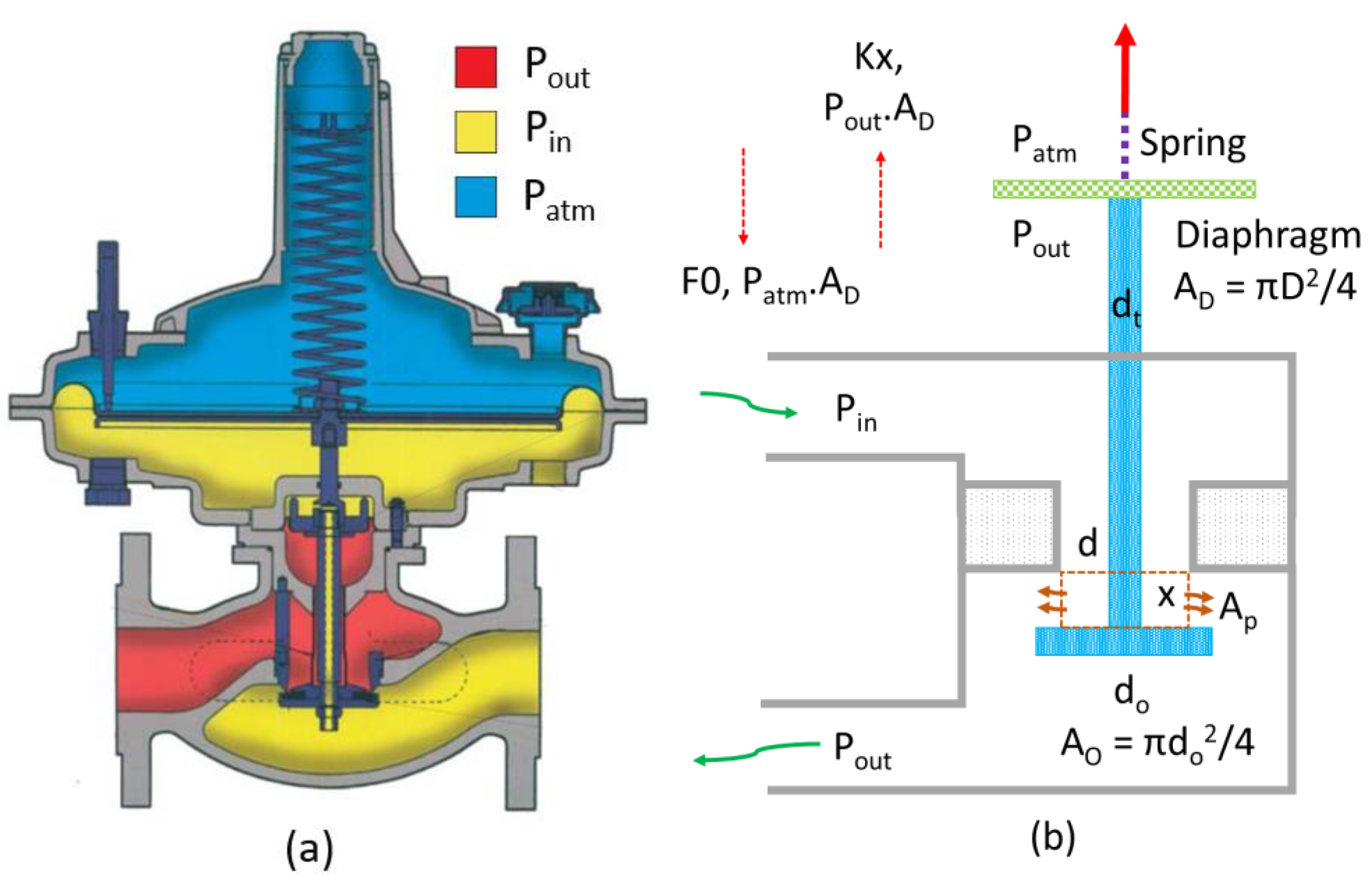
2. Mathematical Model for Spring-Loaded PRs

Figure 2a presents a schematic of a gas PR series 280 (HON 280, [18]). This spring-loaded PR is available in three sizes: 2″ (DN 50), 3″ (DN 80), and 4″ (DN 100). Leo et al. [1] presented a first principles model for the HON 280 that considered the force balance on the valve seat and the diaphragm assembly, as well as the mass and energy balances across the flow chamber. Since PRs have much faster dynamics than downstream gas networks, they reach steady state instantaneously. Hence, it was appropriate to develop a steady-state model for PRs.

This work considered a different geometry of PR valve seats from that in Leo et al. [1] (Figure 2b); However, the model assumptions and equations for the HON 280 PR were the same as those that were used by Leo et al. [1], except for the force balance. The PR model is represented by Equations (1)–(6). The diaphragm and valve seat moved up and down together. Equation (1) presents the force balance on the diaphragm and valve seat assemblies. The chambers above and below the diaphragm were at atmospheric pressure (P_atm) and P_out, respectively. The spring was pre-compressed with an initial force of F0. When the spring was extended (x > 0), then the spring pulled the diaphragm upward. In Equations (1) and (2), P_in is the inlet pressure, K is the spring constant, A_D is the diaphragm area, A_O is the plunger area, A_p is the peripheral flow area, and d is the diameter of the orifice. In Figure 2b, D, d_o and d_t represent the diameters of the diaphragm, plunger, and shaft, respectively.

The mass and energy balances across the flow chamber that were used by Leo et al. [1] are given by Equations (3) and (4). In Equations (3)–(6), T_in is the inlet temperature, T_out is the outlet temperature, m_out is the outlet mass flow, C_d is the orifice discharge coefficient, R is the gas constant, ρ is the density of the gas, γ is the gas heat capacity ratio, μ is the Joule–Thomson expansion coefficient, and N is as defined by Andersen [19].

$$\mathrm{Kx}=\mathrm{F}0+{\mathrm{P}}_{\mathrm{atm}}{\mathrm{A}}_{\mathrm{D}}-{\mathrm{P}}_{\mathrm{out}}{\mathrm{A}}_{\mathrm{D}}+{\mathrm{P}}_{\mathrm{in}}{\mathrm{A}}_{\mathrm{O}}-{\mathrm{P}}_{\mathrm{out}}{\mathrm{A}}_{\mathrm{O}}$$

(1)

$${\mathrm{A}}_{\mathrm{p}}= \mathsf{\pi }\mathrm{dx}$$

(2)

$${\mathrm{T}}_{\mathrm{out}}={\mathrm{T}}_{\mathrm{in}}-\mathsf{\mu }\left({\mathrm{P}}_{\mathrm{in}}-{\mathrm{P}}_{\mathrm{out}}\right)$$

(3)

$${\mathrm{m}}_{\mathrm{out}}={\mathrm{C}}_{\mathrm{d}}{\mathrm{A}}_{\mathrm{p}}{\mathrm{NP}}_{\mathrm{in}}\sqrt{\mathsf{\gamma }}{\left[2/\left(\mathsf{\gamma }+1\right)\right]}^{\left(\mathsf{\gamma }+1\right)/2\left(\mathsf{\gamma }-1\right)}/\sqrt{{\mathrm{RT}}_{\mathrm{in}}}$$

(4)

$$\mathrm{N}=\{\begin{array}{cc}1& {\mathrm{if} \mathrm{P}}_{\mathrm{out}}/{\mathrm{P}}_{\mathrm{in}}\le {\left(\frac{2}{\mathsf{\gamma }+1}\right)}^{\mathsf{\gamma }/\left(\mathsf{\gamma }-1\right)} \\ \sqrt{\frac{{\left(\frac{{\mathrm{P}}_{\mathrm{out}}}{{\mathrm{P}}_{\mathrm{in}}}\right)}^{2/\mathsf{\gamma }}-{\left(\frac{{\mathrm{P}}_{\mathrm{out}}}{{\mathrm{P}}_{\mathrm{in}}}\right)}^{\left(\mathsf{\gamma }+1\right)/\mathsf{\gamma }}}{\left(\frac{\mathsf{\gamma }-1}{2}\right){\left(\frac{2}{\mathsf{\gamma }-1}\right)}^{\left(\mathsf{\gamma }-1\right)/\left(\mathsf{\gamma }+1\right)}}}& \mathrm{otherwise}\end{array}$$

(5)

$$\mathrm{Q}={\mathrm{m}}_{\mathrm{out}}\times 3600/\mathsf{\rho }$$

(6)

In the PR model, x, T_out, μ, γ, and m_out were unknowns. Equation (1) could be solved to compute the spring extension x. Next, A_p could be calculated using Equation (2), in which μ, γ, and ρ depended on the temperature, pressure, and gas composition (X). Following the work of Leo et al. [1], neural network (NN) models were used to estimate μ, γ, and ρ (Equations (7)–(9)) to avoid the use of the computationally expensive Peng–Robinson equation of state. The ANN models were two-layer feedforward networks with one hidden layer and an output layer. In total, 10000 data points were generated for the temperature, pressure, and composition using Latin hypercube sampling. Interested readers are referred to Leo et al. [1] for more details on the ANNs. Equation (3) could be solved iteratively to obtain T_out and μ. Then, m_out was computed using Equations (4) and (6) was used to calculate the hourly volumetric flow through the PR.

$$\mathsf{\mu }={ \mathrm{f}}_{\mathrm{NN}}\left({\mathrm{P}}_{\mathrm{out}},{ \mathrm{T}}_{\mathrm{out}},\mathrm{X}\right)$$

(7)

$$\mathsf{\gamma }={ \mathrm{f}}_{\mathrm{NN}}\left({\mathrm{P}}_{\mathrm{out}},{ \mathrm{T}}_{\mathrm{out}},\mathrm{X}\right)$$

(8)

$$\mathsf{\rho }={ \mathrm{f}}_{\mathrm{NN}}\left({\mathrm{P}}_{\mathrm{out}},{ \mathrm{T}}_{\mathrm{out}},\mathrm{X}\right)$$

(9)

In the mathematical models for spring-loaded (Equations (1)–(6)) and lever-type (Equations (3)–(6) and (10)–(15)) PRs, Equation (3) required most of the computation time. In this equation, there were two unknowns (T_out and μ). The initial value of T_out was assumed to estimate μ using the neural network model (Equation (7)). After that, the μ value was used to compute T_out by solving Equation (3). When the assumed T_out value (that was used to estimate μ in the neural network model) and the computed T_out value (that was obtained after solving Equation (3)) were within the threshold limits, they were used as the final values of T_out and μ.

In this study, the gas mixture that flowed through the PR was about 60% hydrogen, 12% methane, 1% ethane, 4.2% pentane, 4% CO, 17% CO₂, 3.8% N₂, and 1% O₂. It was found that T_out was very close to T_in. Hence, the first principles (PR) models were simplified by assuming T_out = T_in. With hundreds of PRs and hundreds of thousands of data samples for each regulator, this simplification to the mathematical models could significantly reduce computation time.

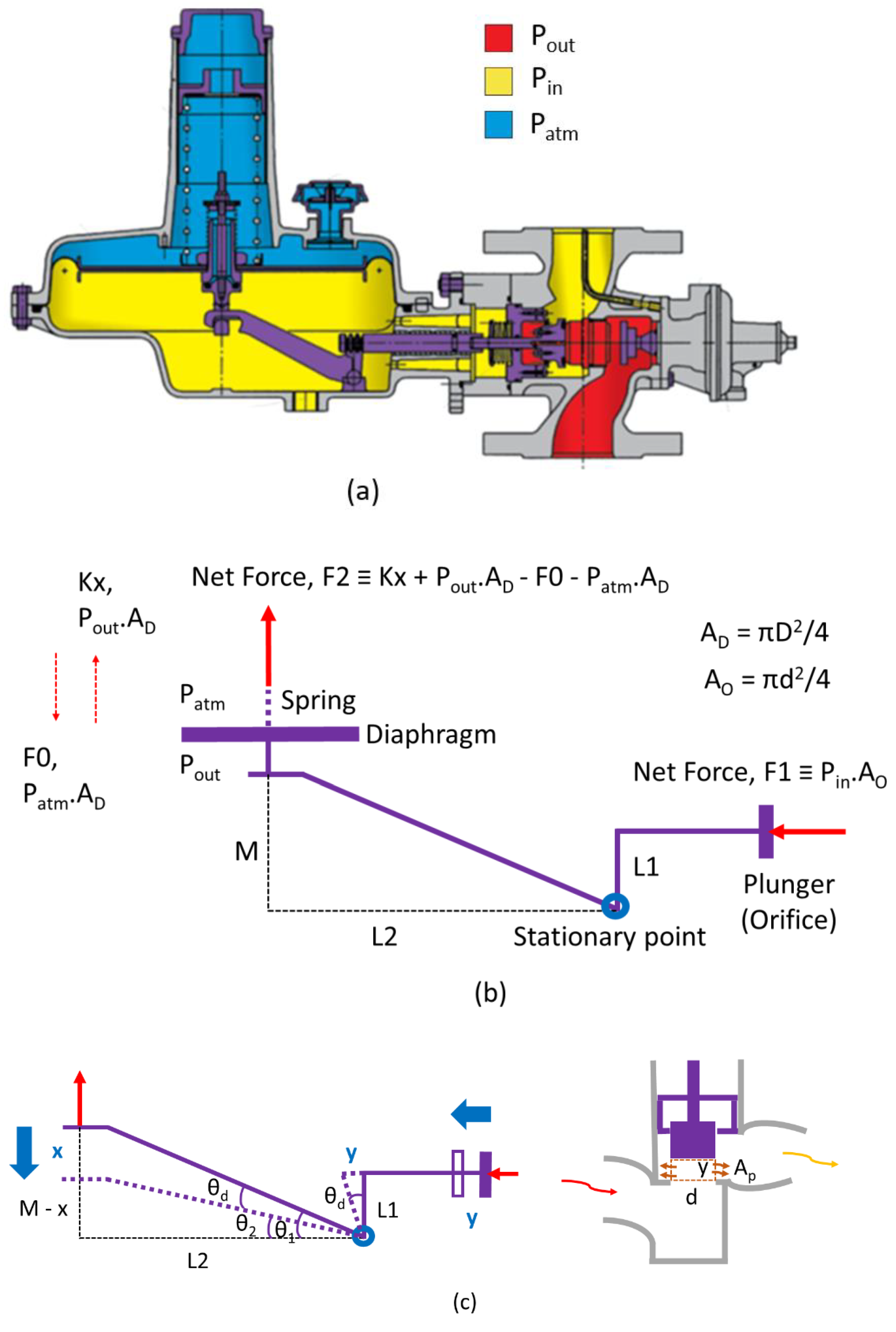
3. Mathematical Model for Lever-Type PRs

Figure 3a presents a schematic of a gas PR series 277 (HON 277). This lever-type PR is available in a 2″ size and is used as a service regulator. The working mechanisms of the HON 277 and HON 280 PRs are very different. The HON 277 PR has a lever between the diaphragm and plunger.

Figure 3b shows the torque balance for this PR. F1 is the force on the plunger that is due to the inlet gas pressure, whereas F2 is the net force on the diaphragm. Equation (10) presents the torque balance around the stationary point in Figure 3b. This equation could be solved to obtain the value of the spring extension (x). For a given value of x, the plunger displacement (y) could be calculated using Equations (11)–(14). Here, Equation (11) provided the initial angle (θ₁) of the lever when x = 0. The final angle (θ₂) of the lever for x was determined using Equation (12). Additionally, θ_d represents the angular movement of the lever that corresponded to the spring extension x (Equation (13) and Figure 3c). The displacement of the plunger could be computed using Equation (14). Finally, the peripheral flow area (A_p) is given by Equation (15).

The mass and energy balances across the flow chamber were the same for both regulators. The complete mathematical model for the lever-type PR contained Equations (3)–(6) and (10)–(15). The solution procedure was also the same for both models.

$$\left(\mathrm{Kx}+{\mathrm{P}}_{\mathrm{out}}{\mathrm{A}}_{\mathrm{D}}-{\mathrm{F}}_0-{\mathrm{P}}_{\mathrm{atm}}{\mathrm{A}}_{\mathrm{D}}\right){\mathrm{L}}_2={\mathrm{P}}_{\mathrm{in}}{\mathrm{A}}_{\mathrm{o}}{\mathrm{L}}_1$$

(10)

$${\mathsf{\theta }}_1={\tan }^{-1}\left(\mathrm{M}/{\mathrm{L}}_2\right)$$

(11)

$${\mathsf{\theta }}_2={\tan }^{-1}\left(\left[\mathrm{M}-\mathrm{x}\right]/{\mathrm{L}}_2\right)$$

(12)

$${\mathsf{\theta }}_{\mathrm{d}}={ \mathsf{\theta }}_1-{ \mathsf{\theta }}_2$$

(13)

$$\mathrm{y}={ \mathrm{L}}_1\tan \left({\mathsf{\theta }}_{\mathrm{d}}\right)$$

(14)

$${\mathrm{A}}_{\mathrm{p}}= \mathsf{\pi }\mathrm{dy}$$

(15)

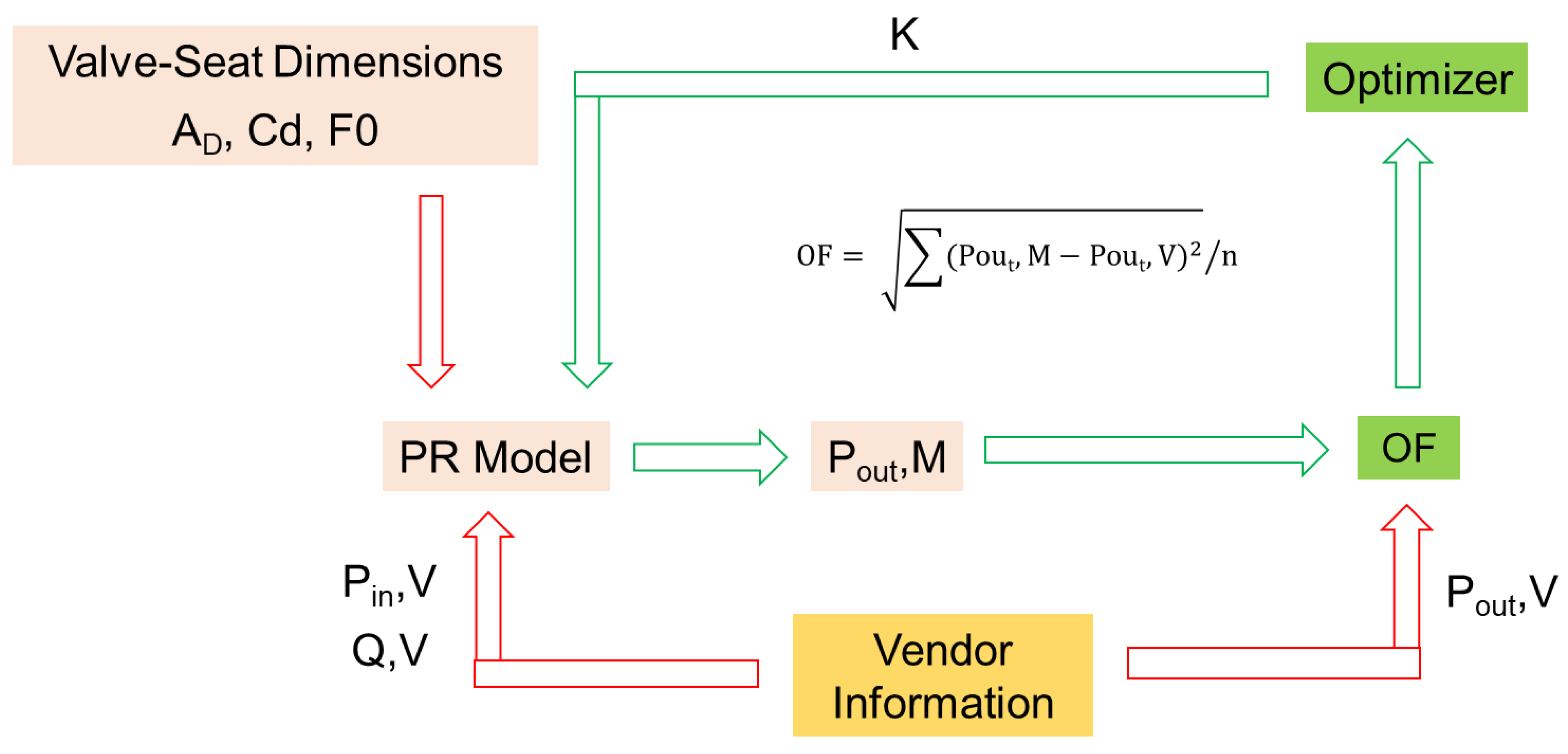
4. Model Parameters

Table 1. The dimensions and model parameters for the two PRs.

Spring-Loaded PR				Lever-Type PR
	4″	3″	2″		2″ SR
dt (m)	0.019	0.0141	0.0145	L1 (m)	0.026
d (m)	0.0998	0.063	0.0497	L2 (m)	0.095
do (m)	0.112	0.088	0.06	M (m)	0.042
D (m)	0.32	0.296	0.272	d (m)	0.032
				D (m)	0.239
Cd	0.87	0.87	0.87	Cd	0.87
Pout,SP (kPa)	15	15	15	Pout,SP (kPa)	17
F0 (N)	120.6	103.2	87.2	F0 (N)	76.3
K (N/m)	51,000	38,800	26,200	K (N/m)	3,790

provides the dimensions of the regulators (d_t, d, d_o, D, L1, L2, and M). In this work, a C_d (coefficient of discharge) of 0.87 was used. The initial force on the spring (F0) was computed using Equation (16). It required set points for ${\mathrm{P}}_{\mathrm{out}}$ and the diaphragm area. To estimate the spring constant (K), the vendor data were used. Table S1 in the Supplementary Materials presents the vendor data (P_in, P_out, and flow) for all of the PRs. Figure 4 shows the algorithm of the optimization-based methodology that was used to estimate K. The optimizer (fmincon in MATLAB) provided the initial K for the first principles (PR) model. The model used P_in and flow data from the vendors and other parameters (dimensions, A_D, Cd, and F0, as shown in Table 1) to predict P_out. An objective function (OF) was calculated using the P_out value that was predicted by the model and the P_out value that was predicted by the vendor, as shown in Figure 4. The optimizer decided on the next K value using this objective function value. The optimization search was terminated after converging to a final K value that minimized the objective function.

$$\mathrm{F}0={ \mathrm{P}}_{\mathrm{out}, \mathrm{SP}}\times {\mathrm{A}}_{\mathrm{D}}$$

(16)

5. Fault Monitoring Methodologies

This section discusses the methodologies that were developed for fault monitoring in PRSs. Firstly, data preprocessing is discussed before addressing the potential faults in PRSs, namely filter choking, valve seat damage, and diaphragm deterioration. In general, gas distributors do not measure flows through PRSs. Furthermore, most gas companies only measure ${\mathrm{P}}_0$ and ${\mathrm{P}}_{\mathrm{out}}$. Figure 5 summarizes the methodologies that were developed to monitor the three faults (filter choking, valve seat damage, and diaphragm deterioration).

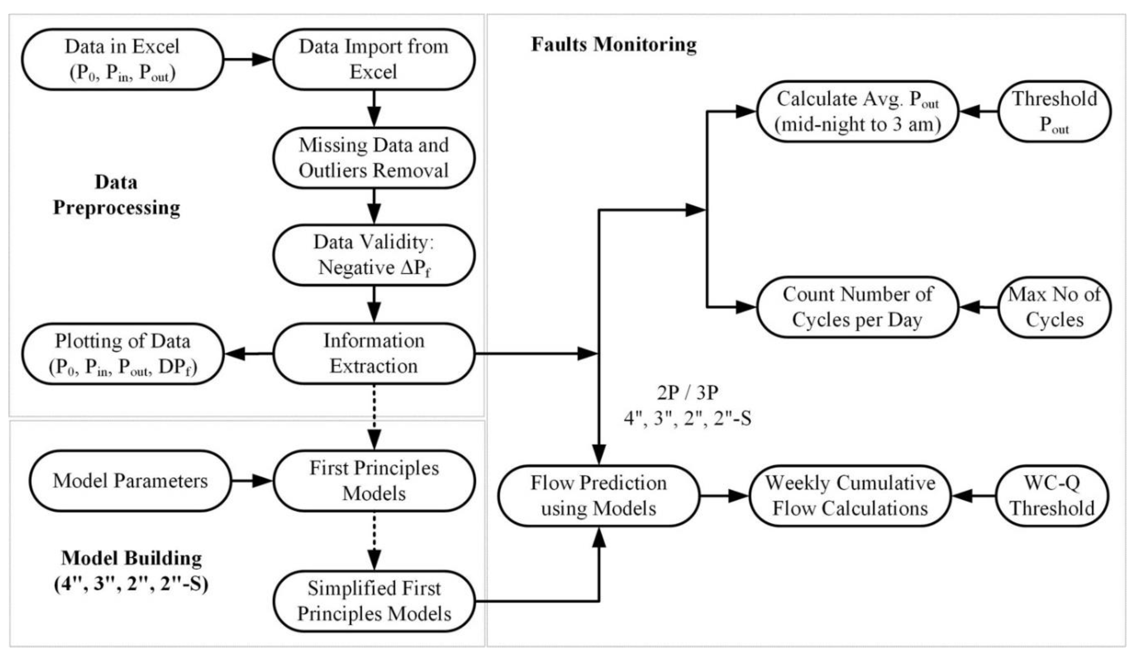
5.1. Data Preprocessing

• Data were imported from Excel into MATLAB. Each regulator had an Excel file with the date, time, inlet pressure (P₀), intermediate pressure (P_in), and outlet pressure (P_out) data. Some did not have P_in data.
• When one pressure value was missing for a data point, then all of its pressure values were replaced by those for the previous data point. A pressure value was considered an outlier when it was more than three standard deviations away from the mean value. Outlier pressure values were replaced by the previous pressure value.
• Data were checked for valid pressure drops across the filter (ΔP_f). The number (SN-ΔP_f) of data samples with negative ΔP_f values was computed. When SN-ΔP_f was lower than 0.1% of the number of all samples, then those faulty pressure values were replaced by the mean values. Otherwise, New P_in = Old P_in − max (ΔP_f).
• Important information was extracted, such as the start and end dates of the data, the number of days of data, and the number of samples for each day.
• Finally, the pressure data were visualized by plotting P₀, P_in, P_out, and ΔP_f against time.

5.2. Filter Choking

As discussed earlier, both spring decay and filter choking cause low pressure in downstream networks. In general, spring decay is much slower than filter choking. For relatively short periods, the spring constant can be assumed to be constant. Hence, filter choking can be considered as the main reason for pressure decrease in downstream networks. An ideal regulator maintains the outlet pressure at P_out,SP for any flow and P_in values. However, P_out decreases with the flow and P_in values (droop curve, [20]) for real regulators.

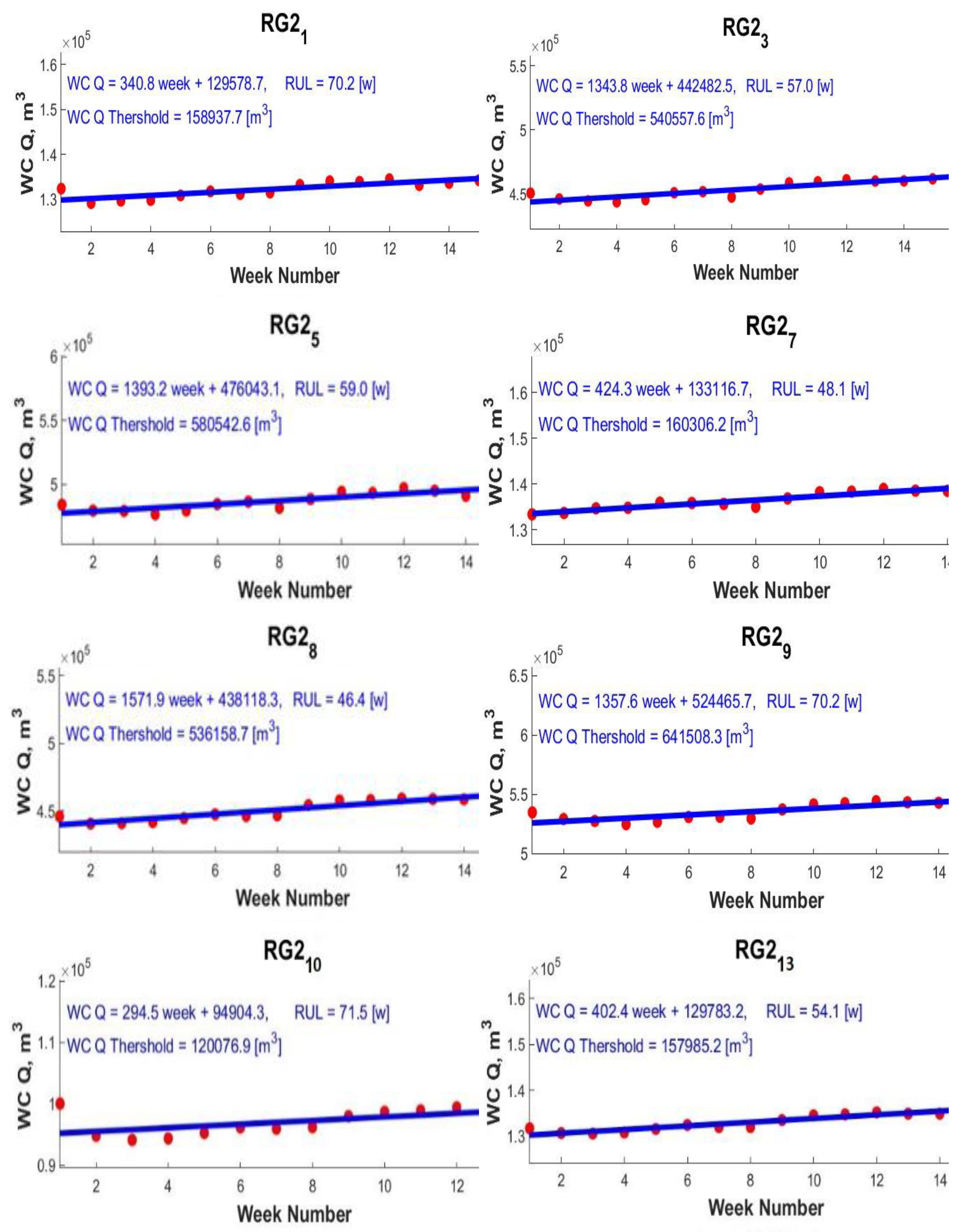
For a constant P₀, P_in decreases as the filter chokes. When the weekly cumulative gas flow (WC-Q) within a network remains nearly the same, then P_out also decreases to compensate for the lower P_in in order to maintain the same WC-Q. Hence, filter choking impacts P_out. However, the model with no filter choking predicted a higher WC-Q value for the measured pressures. Thus, an increase in WC-Q could indicate filter choking. When P_in values were not available, then P₀ values could be used as proxies, and the flow could be estimated using our mathematical model. As shown in Figure S1 (Supplementary Materials), the impact of P_out was more significant than that of P_in on the calculated flow. Hence, the inferences that were drawn were not compromised. Thus, WC-Q was estimated from the data using our simplified mathematical model. The filter RUL was estimated by fitting a line through the estimated WC-Q values. Filter maintenance is recommended when the RUL values exceed an agreed threshold value. The monitoring steps that were involved in our model were as follows:

• Input threshold WC-Q values for the PRs (4″, 3″, 2″, and 2″ SR);
• Calculate gas flows (Q) for all data points using the simplified mathematical model (as discussed in Section 2 and Section 3) Using the model parameters for the 4″, 3″, 2″, and 2″ SR PRs that are presented in Table 1;
• In the absence of P_in data, Q_M,2P = f (PR type, model parameters, P₀, and P_out);
• When P_in is available, Q_M,3P = f (PR type, model parameters, P_in, and P_out);
• PR type: spring-loaded PR or lever-type PR;
• Calculate WC-Q;
• Plot WC-Q against time and obtain the best linear fit;
• From the linear fit, estimate the number of weeks for the current WC-Q to reach the threshold WC-Q. That was the estimate for the filter RUL.

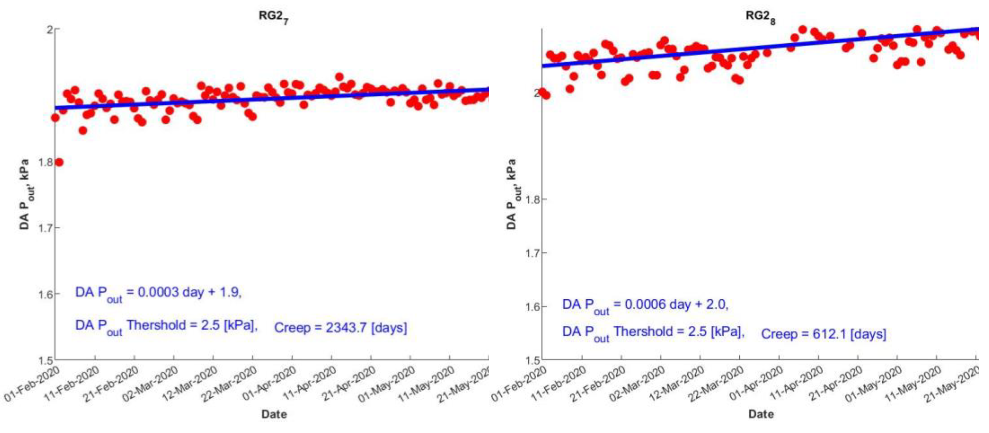
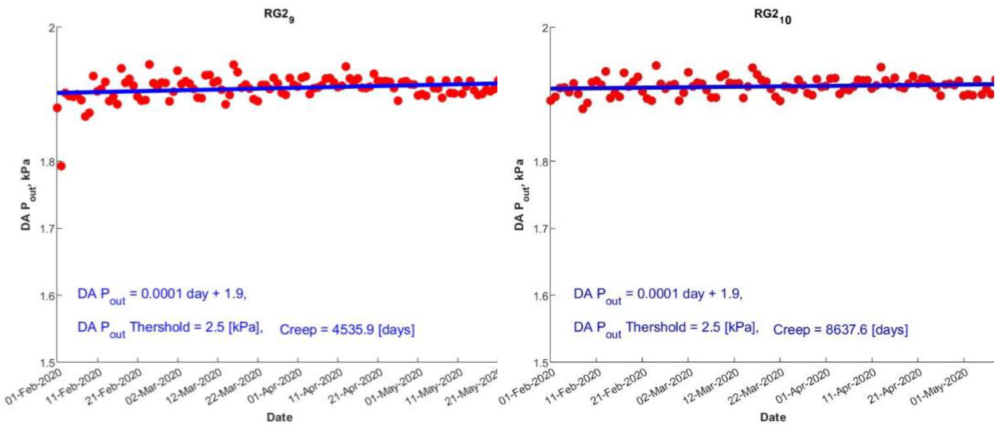
5.3. Valve Seat Damage

The valve seats make repeated contact with the orifices during the operation of PRs. Contaminant particles can also be deposited from various sources, including pipe wear and tear. Damaged valve seats can allow tiny leaks, even when the valves are completely shut. This is known to produce a creep effect. This creep effect manifests as a downstream over-pressure in the network during low demand periods (e.g., around midnight).

After analyzing the available data, we confirmed that low flows could exist in the PRs between 12 am and 3 am. Following the work of Leo et al. [1], the available P_out data for the gas network during this period were checked carefully and were found to be too noisy to reliably determine the daily maximum P_out value. Hence, to minimize the impacts of abrupt fluctuations and sensor noise, the average P_out value was computed for that period. The average P_out value seemed more reliable than the daily P_out value for monitoring valve seat condition.

• Input threshold P_out value for creep effect (valve seat damage);
• For each day, compute the average P_out value from 12 am to 3 am;
• Plot the average P_out against time and obtain the best linear fit;
• Using the linear fit, estimate the number of days needed for the current P_out value to reach the threshold P_out value. That was the estimate for the valve seat RUL.

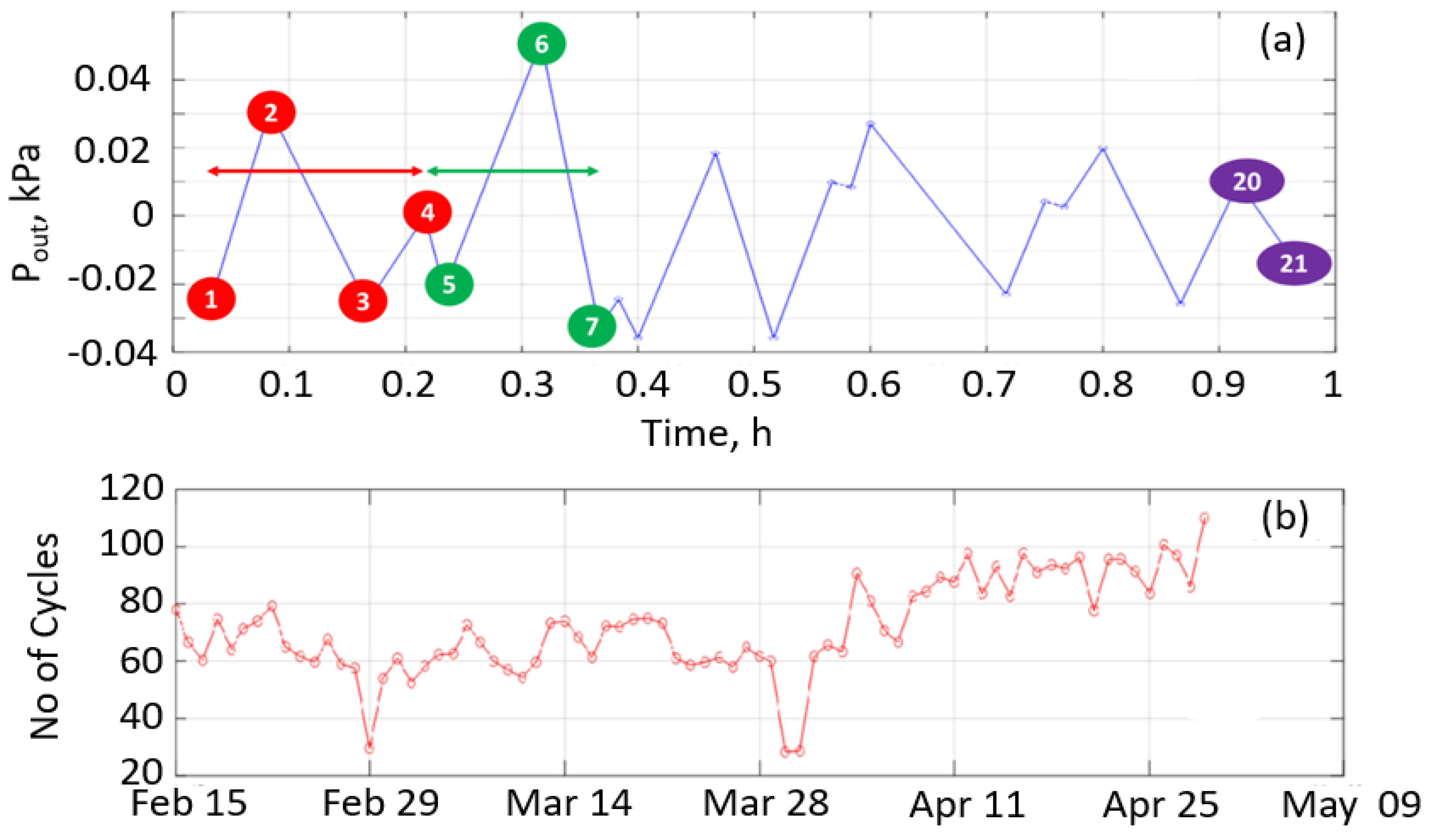
5.4. Diaphragm Malfunction

The diaphragm and valve seat move together to maintain P_out near the set point. When the diaphragm senses a deviation in P_out from the set point, the valve seat moves up or down accordingly. The diaphragm is thus subjected to cyclic stress, which can eventually lead to its fatigue failure. The lifetime of diaphragms is measured using up-down cycles (200,000; [21]). The up-down movement of diaphragm is measured using the spring extension, but it is very difficult to measure the spring extensions in hundreds of regulators.

After closely inspecting the real operational data, we noticed that P_out experienced more fluctuations in small flows around midnight. There can be multiple up-down cycles during each hour of PR operation. Hence, a methodology to count all of the up-down cycles in P_out was developed.

• Detrend P_out data for each hour (Figure S2 in the Supplementary Materials). For this, the linear best fit was subtracted from the raw data to produce a zero mean for the detrended data;
• Find the local minimum and maximum values (Figure S2 in the Supplementary Materials). The local minimum and maximum values were used to identify the data points at which the diaphragm movement changed from upward to downward or from downward to upward;
• Construct up-down cycles using the local minimum and maximum values (Figure 6a);
• Determine the number of cycles per day using (maximum and minimum values − 1)/3 (Figure 6b);
• Compute percentage deterioration in diaphragm condition over a year using Equation (17).

$$\mathrm{Annual} \mathrm{Use} \mathrm{of} \mathrm{a} \mathrm{Diaphragm}=\frac{\mathrm{Number} \mathrm{of} \mathrm{cycles} \mathrm{in} \mathrm{a} \mathrm{year}}{\mathrm{Maximum} \mathrm{number} \mathrm{of} \mathrm{cycles}}\%$$

(17)

6. Results and Discussion

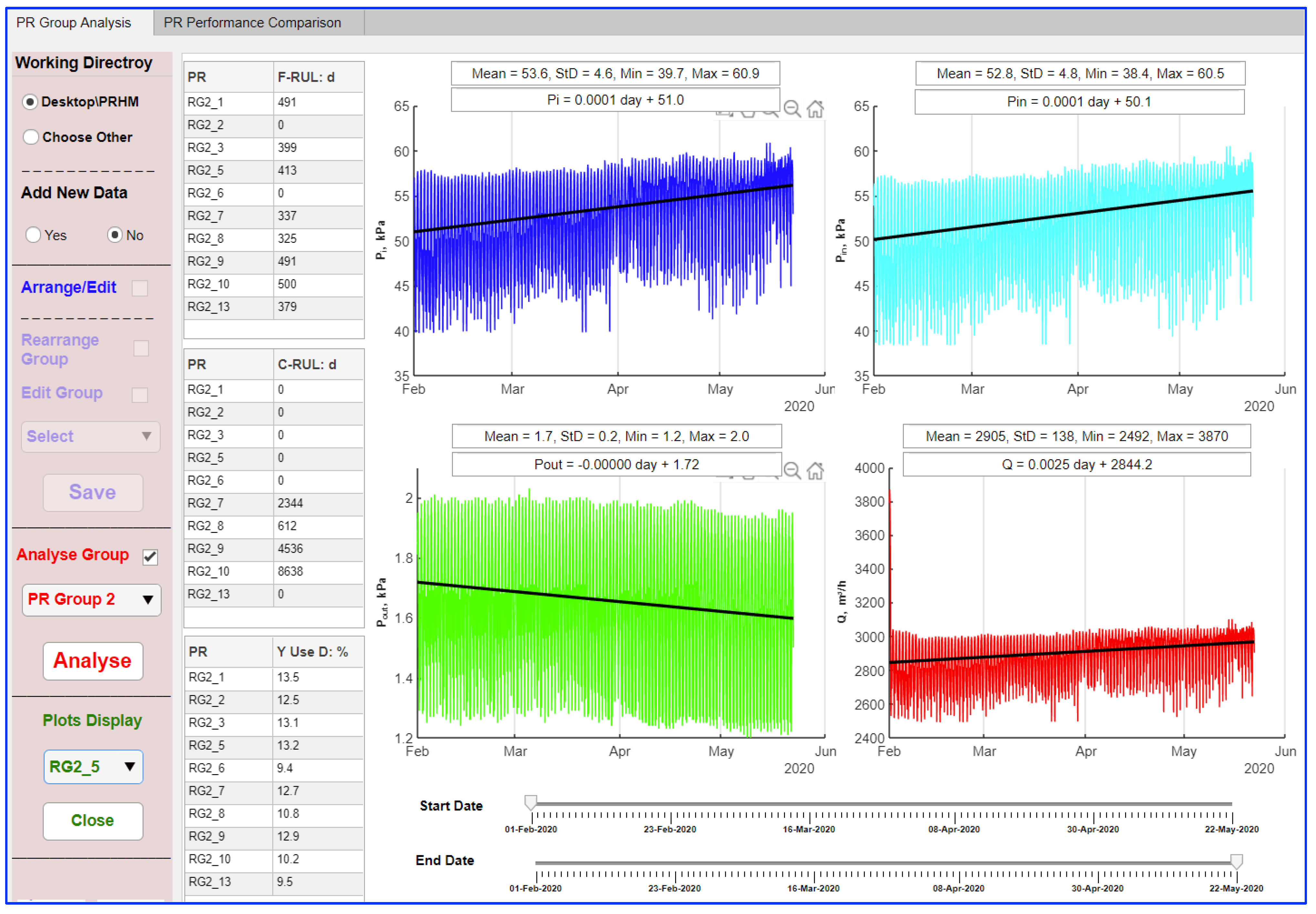
6.1. Pressure Regulator Health Monitor (PRHM) Dashboard

A user-friendly dashboard (the PRHM) was developed to monitor the health of PRs within gas networks. The hundreds of PRs within a network can be divided into groups based on their geographical locations for easier analysis and comparison. Through the PRHM, PR groups can be updated by adding or removing PRs.

The PRHM has two tabs: “Group Analysis” and “Performance Comparison”. The first tab is used to evaluate some or all PRs within a PR group. The second tab is used to analyze and compare the performances of the PRs in different groups. For each PR, data files are updated automatically as needed. The user can choose the start and end dates for the analysis. The GUI of the PRHM is shown in Figure S3 in the Supplementary Materials. The left-hand side of the PRHM (“Working Directory”, “Add New Data”, “Arrange/Edit”, “Analyze Group”, and “Plots Display”) indicates its capabilities. When a particular regulator group is chosen for analysis (e.g., the PR Group 2 in Figure S3 in the Supplementary Materials), then the right-hand side table in the PRHM presents all of the essential information for that group. The data in the table can be modified as needed before starting the analysis. When a regulator is chosen for analysis, then the color of the entire row changes (e.g., in Figure S3 in the Supplementary Materials, in which a color change to yellow is shown).

In this study, the PR Group 2 contained 15 PRs: RG2_1, RG2_2, …, RG2_15. Each PR had data for different dates, as shown in Figure S3 in the Supplementary Materials. In total, 10 of the 15 PRs were chosen for analysis and then the “Analyze Group” button was clicked. In total, there were 404,694 data points for the 10 PRs. The PRHM dashboard showed the progress of calculations and error messages (when applicable). In the case of error messages, it provided suggestions for how to resolve the errors. The PRHM took about 7 minutes to analyze the 10 PRs using a Windows workstation with 16 GB of RAM and a i7 7700 CPU at 3.60 GHz. After completing the analysis, the PRHM showed three tables for the filter RUL, the creep effect (valve seat) RUL, and the annual diaphragm usage (Figure 7). Users could choose a PR from the drop-down list under the “Plots Display” menu to visualize the pressures and flows. In Figure 7, the inlet pressure, intermediate pressure, outlet pressure, and gas flow data are shown for RG2_5. The sliders below the plots could be used to adjust their display time windows.

All of the results from the analyses were automatically saved in different folders. Old results were removed after one month. Each regulator group had a separate folder for their results (e.g., “PR Group 2″ was the name of the folder for PR Group 2). Each group’s folder had five subfolders for the various plots: (1) the daily number of data points for each PR; (2) the inlet, intermediate, and outlet pressure data and the pressure difference across each filter; (3) the daily average flow through each PR; (4) the weekly cumulative flow through each PR; and (5) the daily average P_out from 12 am to 3 am for each PR.

6.2. Filter Choking

As explained previously, the weekly cumulative flow through a PR is used to monitor filter choking. Figure 8 presents the plots for the weekly cumulative flow against time for eight selected PRs (RG2_1, RG2_3, RG2_5, RG2_7, RG2_8, RG2_9, RG2_10, and RG2_13). For these PRs, the weekly cumulative flow increased monotonically.

The linear regression line is shown in each plot, along with the slope and intercept. Table S2 in the Supplementary Materials shows the confidence intervals for the intercept and slope of the fitted lines. The confidence intervals were calculated for fitted lines with positive slopes and their parameters were statistically significant. The threshold value of the weekly cumulative flow that was used to calculate the RUL was 20% above the average weekly flow that was predicted by the model for the first week. The resultant RUL values are shown in Figure 8 and

Table 2. The estimated RUL values for the filter and the valve seat and the annual diaphragm usage for the different PRs.

PR Name	Filter RUL	Valve Seat RUL	Annual Diaphragm Usage
	(d)	(d)	(%)
RG2_1	491	0	13.5
RG2_2	0	0	12.5
RG2_3	399	0	13.1
RG2_5	413	0	13.2
RG2_6	0	0	9.4
RG2_7	337	2344	12.7
RG2_8	325	612	10.8
RG2_9	491	4536	12.9
RG2_10	500	8638	10.2
RG2_13	379	0	9.5

. For RG2_2 and RG2_6, the linear regression lines had negative slopes due to the poor quality of the pressure data. In these cases, the dashboard did not display any filter RUL estimations.

6.3. Valve Seat Damage (Creep Effect)

Figure 9 presents the average P_out values (12 am to 3 am) for several days. The average daily P_out value only increased for RG2_7, RG2_8, RG2_9, and RG2_10. The P_out values are expected to increase for damaged valve seats; hence, it could be concluded that the other PRs had no issues with their valve seats. The fitted lines for various PRs are shown in Figure 9. Table S3 in the Supplementary Materials shows the confidence intervals for the intercept and slope of the lines. The confidence intervals were only computed for lines with positive slopes and the line parameters were statistically significant (except RG2_10, which had a lower confidence interval because the slope was negative). The threshold value of the average daily P_out was 2.5 kPa. The RUL for each valve seat can be seen in Figure 9 and Table 2.

6.4. Diaphragm Malfunction

For the selected PRs in PR Group 2, Figure S5 in the Supplementary Materials shows the daily diaphragm cycles. In general, diaphragms have a lifetime of about 10 years or 200,000 cycles [21]. The annual diaphragm usage (i.e., the number of diaphragm cycles over one year expressed as a percentage of the number of cycles over the lifetime of the diaphragm) of the PRs are presented in Table 2. The 10 diaphragms completed around 11.8% of their lifetime cycles over one year. This correlated well with the expected lifetime of 10 years, but earlier replacement could be required (depending on when the diaphragm was last changed).

7. Conclusions

In this work, mathematical models for spring-loaded PRs and lever-type PRs were developed. As gas distribution networks can have hundreds of PRs, the mathematical models were simplified for faster computation. Methodologies for monitoring filter choking, valve seat damage, and diaphragm deterioration were developed for PRs, which demonstrated high reliability and accuracy. The methodologies combined the mathematical models with the available experimental pressure data that were measured upstream and downstream of regulators to infer the health of various components within PRSs. It was demonstrated that filter choking, which occurs relatively rapidly, could be monitored by tracking increases in estimated weekly cumulative flows through the PRs. Similarly, the development of valve seat damage in the regulators, which is a slow process, could be assessed over a long period of time by observing creeping increases in average daily P_out values for a period in the day when no flow was expected. Diaphragm condition could be monitored by the number of up-down cycles using the P_out values. The methodologies for monitoring these faults were extended to estimate the RUL of each component. For industrial users, a user-friendly PRHM dashboard was created to provide a one-stop platform for monitoring the health of PRs within gas networks and planning the timely maintenance of deteriorating components. This work could help toward increasing the system reliability of legacy systems and ensuring uninterrupted gas supplies for customers.

References

- Leo, M.B.; Dutta, A.; Farooq, S.; Karimi, I.A. Simulation and health monitoring of a pressure regulating station. Comput. Chem. Eng. 2020, 139, 106824. [Google Scholar] [CrossRef]
- Rao, H.N.; Xiang, L.R.; Karimi, I.A. Modelling pressure regulators using operational data. In Foundations of Computer Aided Process Operations/Chemical Process Control; San Antonio, Texas. 2017. Available online: https://folk.ntnu.no/skoge/prost/proceedings/focapo-cpc-2017/FOCAPO-CPC%202017%20Contributed%20Papers/106_FOCAPO_Contributed.pdf (accessed on 2 April 2021).
- Afshari, H.H.; Zanj, A.; Novinzadeh, A.B. Dynamic analysis of a nonlinear pressure regulator using bondgraph simulation technique. Simul. Model. Pract. Theory 2010, 18, 240–252. [Google Scholar] [CrossRef]
- Dasgupta, K.; Karmakar, R. Modelling and dynamics of single-stage pressure relief valve with directional damping. Simul. Model. Pract. Theory 2002, 10, 51–67. [Google Scholar] [CrossRef]
- Nabi, A.; Dayan, J. Dynamic model for a dome-loaded pressure regulator. J. Dyn. Syst. Meas. Control. Trans. ASME 2000, 122, 290–297. [Google Scholar] [CrossRef]
- Rami, E.G.; Jean-Jacques, B.; Pascal, G.; François, M. Stability study and modelling of a pressure regulating station. Int. J. Press. Vessel. Pip. 2005, 82, 51–60. [Google Scholar] [CrossRef]
- Zafer, N.; Luecke, G.R. Stability of gas pressure regulators. Appl. Math. Model. 2008, 32, 61–82. [Google Scholar] [CrossRef]
- Wang, X.S.; Cheng, Y.H.; Peng, G.Z. Modeling and self-tuning pressure regulator design for pneumatic pressure load systems. Control Eng. Pract. 2007, 15, 1161–1168. [Google Scholar]
- Prescott, S.L.; Ulanicki, B. Dynamic modeling of pressure reducing valves. J. Hydraul. Eng. 2003, 129, 804–812. [Google Scholar]
- Shahani, A.R.; Esmaili, H.; Aryaei, A.; Mohammadi, S.; Najar, M. Dynamic simulation of a high-pressure regulator. JCARME 2011, 1, 17–28. [Google Scholar]
- Ramzan, M.; Maqsood, A. Dynamic modeling and analysis of a high pressure regulator. Math. Probl. Eng. 2016, 2016, 1307181. [Google Scholar] [CrossRef]
- Patil MGand Barjibhe, R.B. Flow analysis of gas pressure regulator by numerical and experimental method. Int. Res. J. Eng. Technol. (IRJET) 2018, 5, 747–752. [Google Scholar]
- Yinxing, D.; Huaixiu, W.; Yahui, W.; Fangwen, C. Research on fault diagnosis algorithm of gas pressure regulator based on compressed sensing theory. In Proceedings of the 2017 29th Chinese Control and Decision Conference, Chongqing, China, 28–30 May 2017. [Google Scholar]
- Yun, A.; Yahui, W.; Yuexiao, L. Research on gas pressure regulator fault diagnosis based on deep confidence network (DBN) Theory. In Proceedings of the 2017 Chinese Automation Congress, Jinan, China, 20–22 October 2017. [Google Scholar]
- Song, Y.; Wang, Y. A fault detection method for gas pressure regulators based on improved dynamic canonical correlation analysis. In Proceedings of the 2021 33rd Chinese Control and Decision Conference, Kunming, China, 22–24 May 2021. [Google Scholar]
- Jia, J.; Wang, B.; Ma, R.; Deng, Z.; Fu, M. State monitoring of gas regulator station based on feature selection of improved grey relational analysis. IEEE Internet Things J. 2022. [Google Scholar] [CrossRef]
- Wang, B.; Jia, J.; Deng, Z.; Fu, M. A state monitoring method of gas regulator station based on evidence theory driven by time-domain information. IEEE Trans. Ind. Electron. 2022, 69, 694–702. [Google Scholar] [CrossRef]
- RMG by Honeywell. Gas Pressure Regulator Technical Datasheet. Available online: https://www.honeywellprocess.com/library/marketing/brochures/HON_280-284%20Brochure.pdf (accessed on 2 April 2021).
- Andersen, B.W. The Analysis and Design of Pneumatic Systems; Wiley: New York, NY, USA, 1967. [Google Scholar]
- Emerson. The Industry Standard for Pressure Regulators. Available online: https://www.emerson.com/documents/automation/catalog-regulators-mini-catalog-fisher-en-125484.pdf (accessed on 15 October 2019).
- Sutar, S.S.; Kunbade, P.R.; Jamadade, S.S. Fatigue life estimation of pressure reducing valve diaphragm. IJEAT 2015, 4, 180–188. [Google Scholar]