
Stator Curvature Optimization and Analysis of Axial Hydraulic Vane Pumps

Abstract
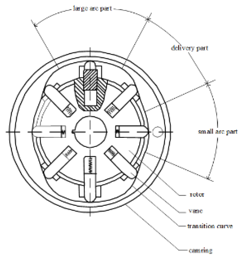
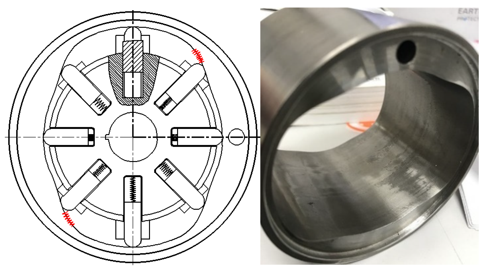
:1. Introduction
2. Establishment of the Blade Force Model’s Objective Function
- (1)
- The centrifugal force of the blade as a function of the rotation angle [19] is shown in Equation (1).
- (2)
- The spring force on the blade as a function of the angle of rotation is shown in Equation (2).
- (3)
- The inertia force on the blade as a function of the angle of rotation is shown in Equation (3).
- (4)
- The frictional force between the blade and the inner cavity of the stator as a function of the rotation angle is shown in Equation (4).
- (5)
- The Coe-type inertia force oonthe blade as a function of the rotation angle [20] is shown in Equation (5).
- (6)
- The viscous friction force on the blade as a function of the rotation angle is shown in Equation (6).
- (7)
- The contact reaction force oonthe blade by the rotor is shown in Equation (7) as a function of the rotation angle.
- (8)
- The hydraulic pressure on the blade as a function of the turning angle is shown in Equation (8).
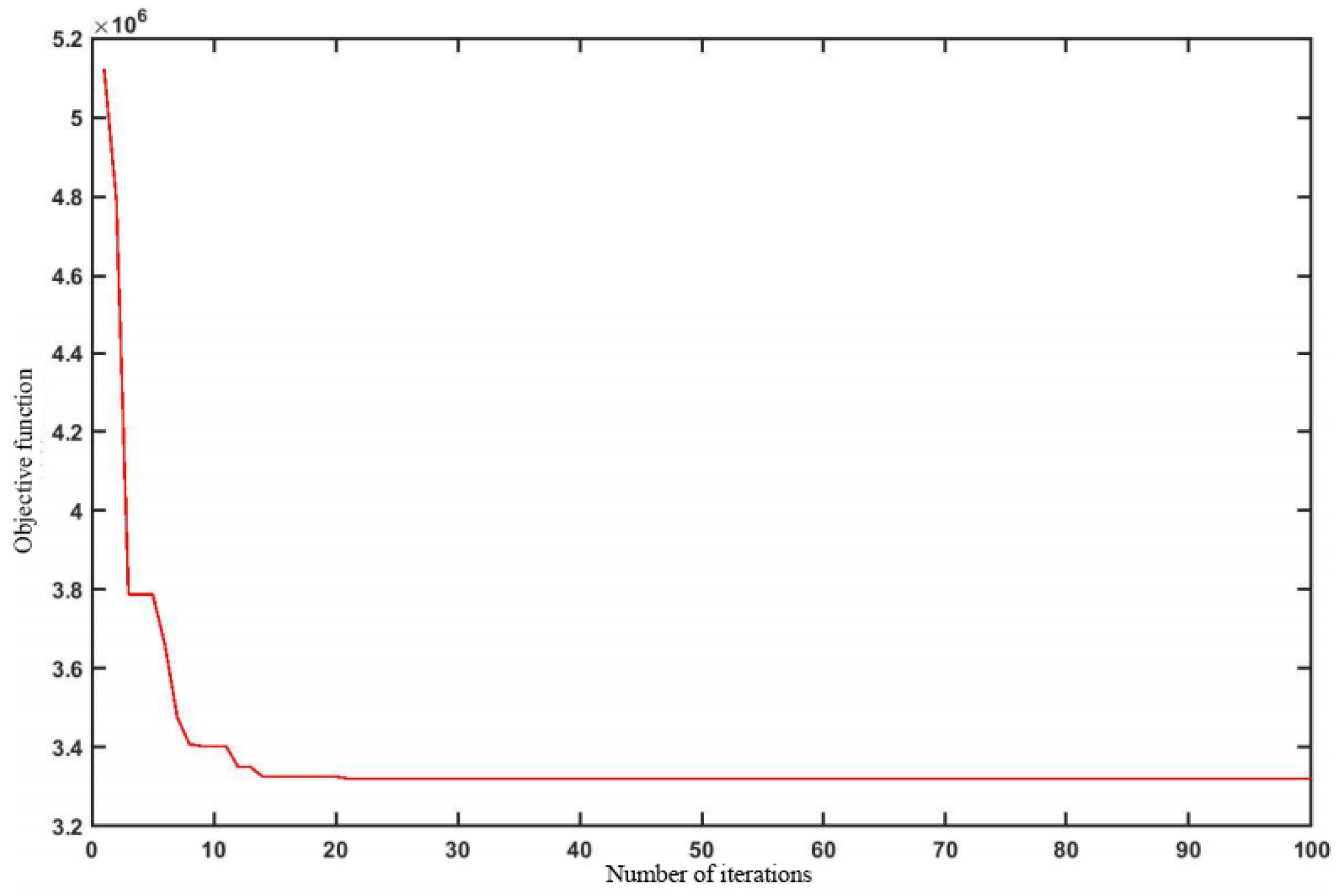
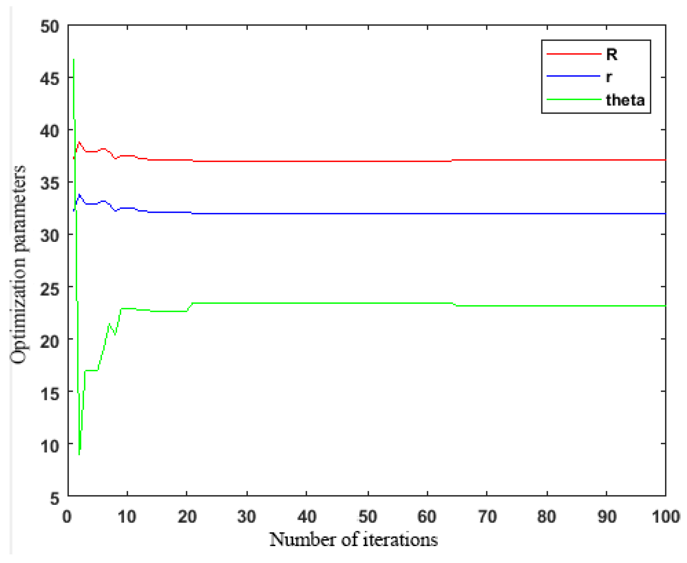
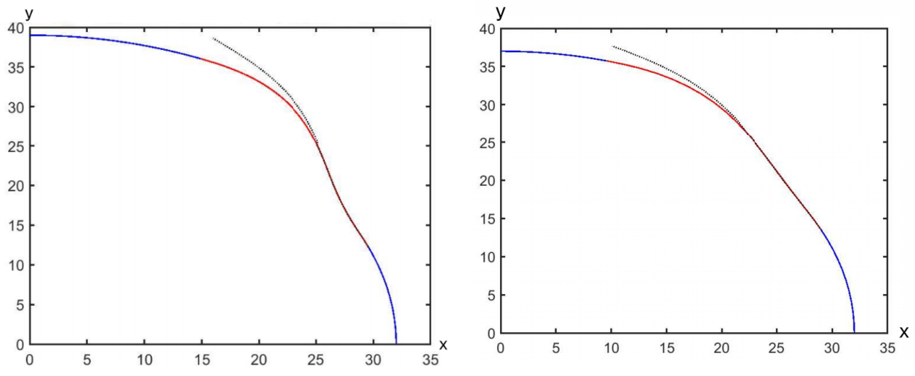
3. Stator Inner Cavity Curve Length and Radius Optimization
- (1)
- When R − r = 1, the minimum value of the objective function is 4.8298 × 10⁶, at which time R = 33, r = 32, θ = 26.65°.
- (2)
- When R − r = 2, the minimum value of the objective function is 4.4148 × 10⁶, when R = 34, r = 32, θ = 24.56°.
- (3)
- When R − r = 3, the minimum value of the objective function is 4.0240 × 10⁶, when R = 35, r = 32, θ = 23.71°.
- (4)
- When R − r = 4, the minimum value of the objective function is 3.6583 × 10⁶, when R = 36, r = 32, θ = 22.90°.
- (5)
- When R − r = 5, the minimum value of the objective function is 3.3217 × 10⁶, when R = 37, r = 32, θ = 23.13°.
- (6)
- When R − r = 6, the minimum value of the objective function is 3.4313 × 10⁶, when R = 38, r = 32, θ = 22.14°.
4. Results
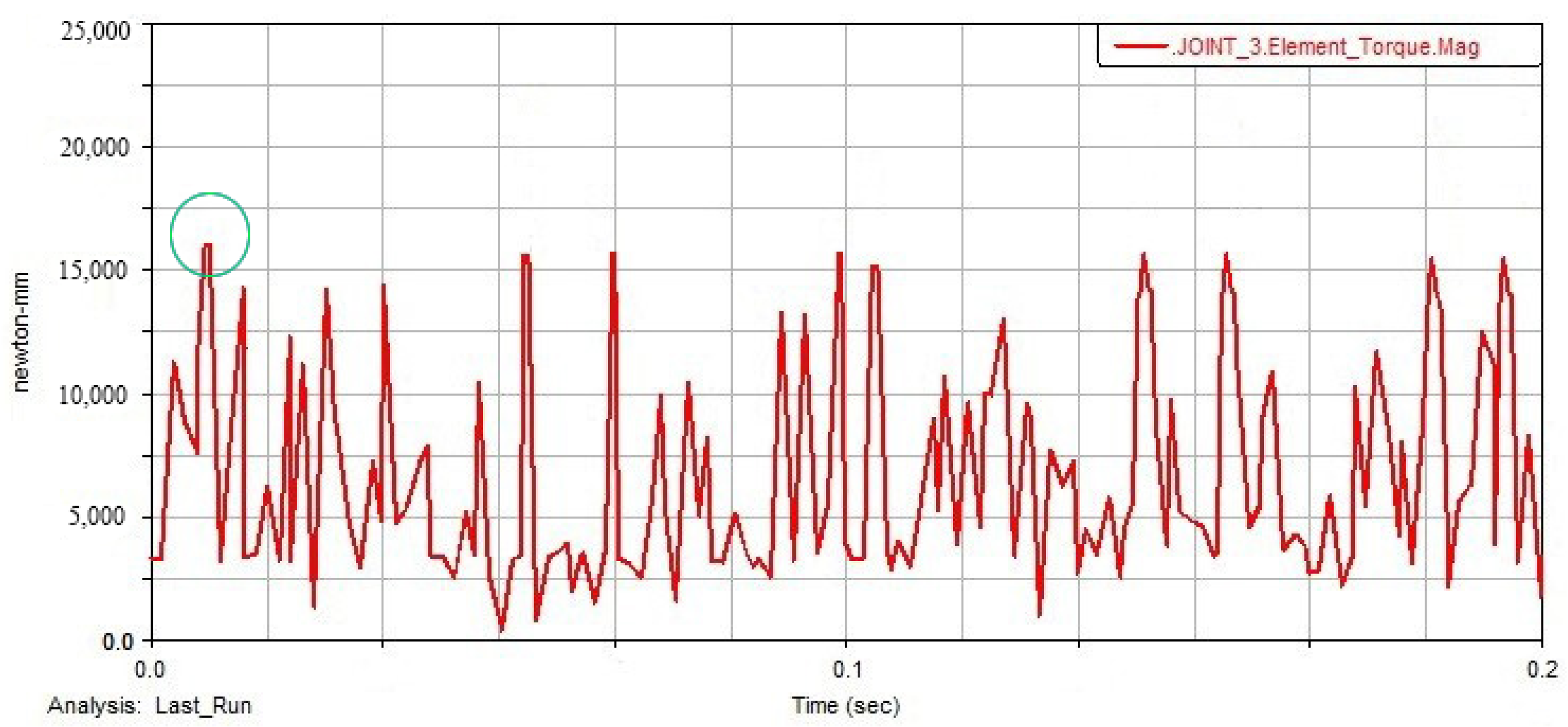
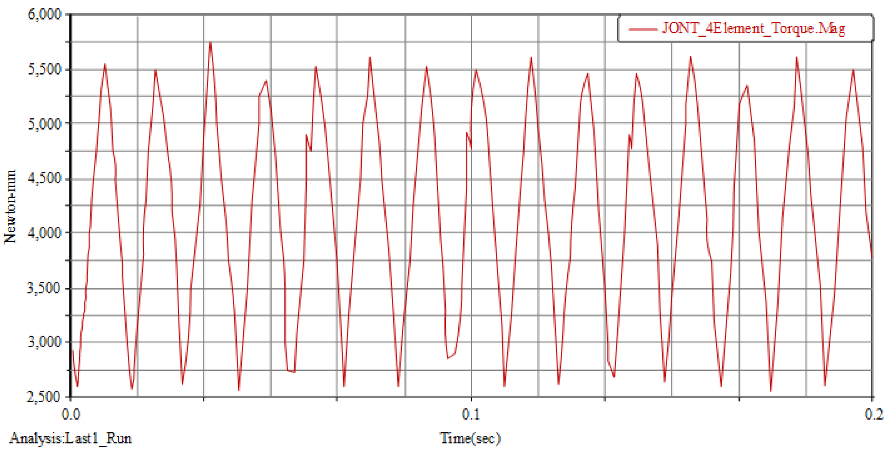
- (1)
- Spindle torque curve before and after stator cavity length to radius ratio optimization.
- (2)
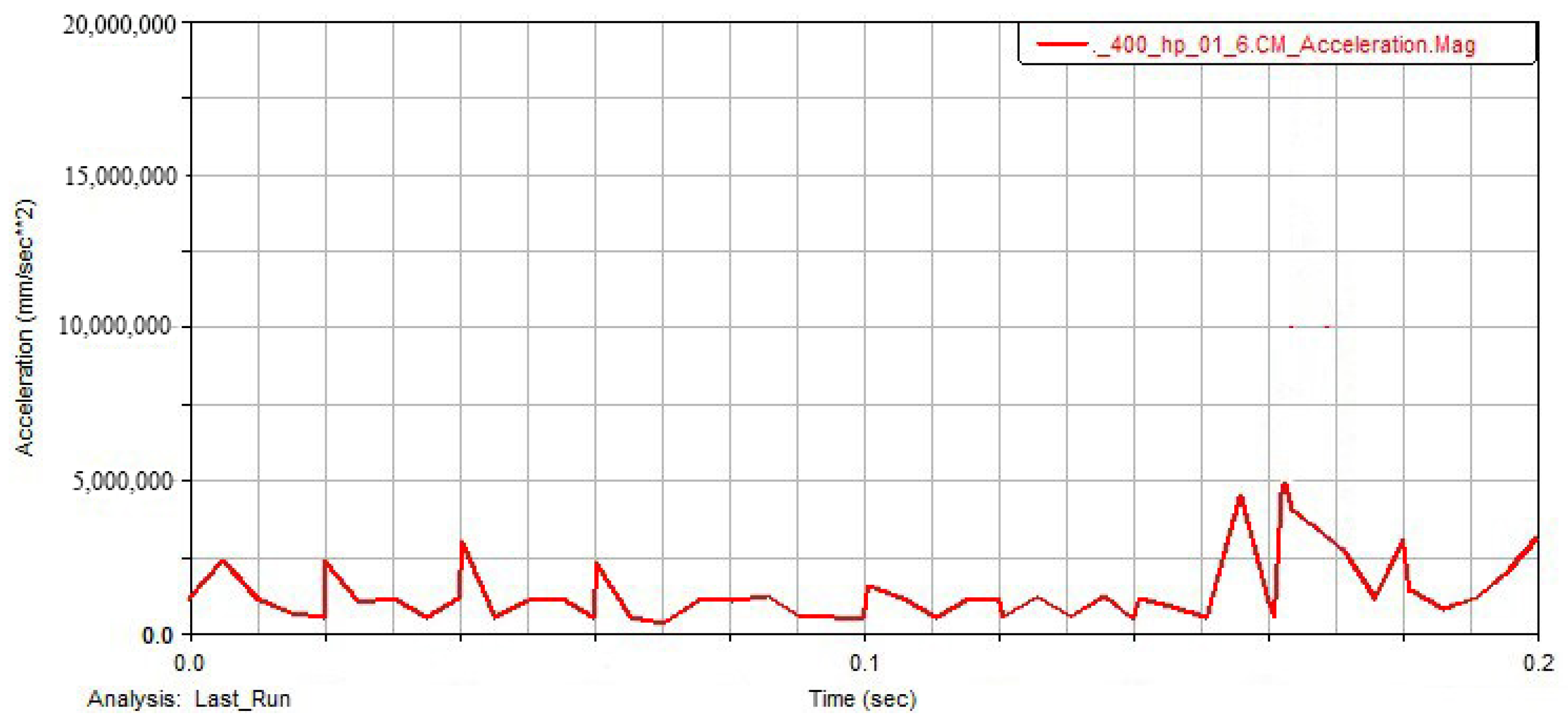
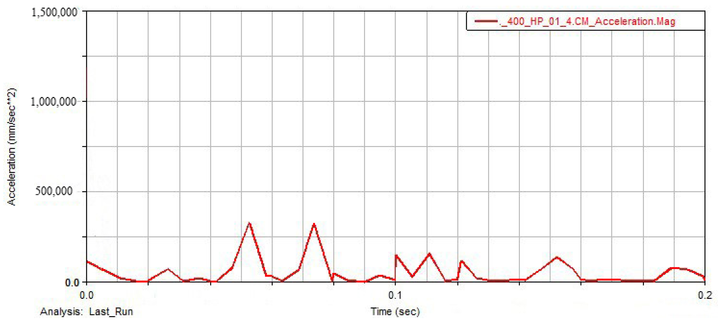
- Slider acceleration curves before and after optimizing stator cavity length to radius ratio.
- (3)
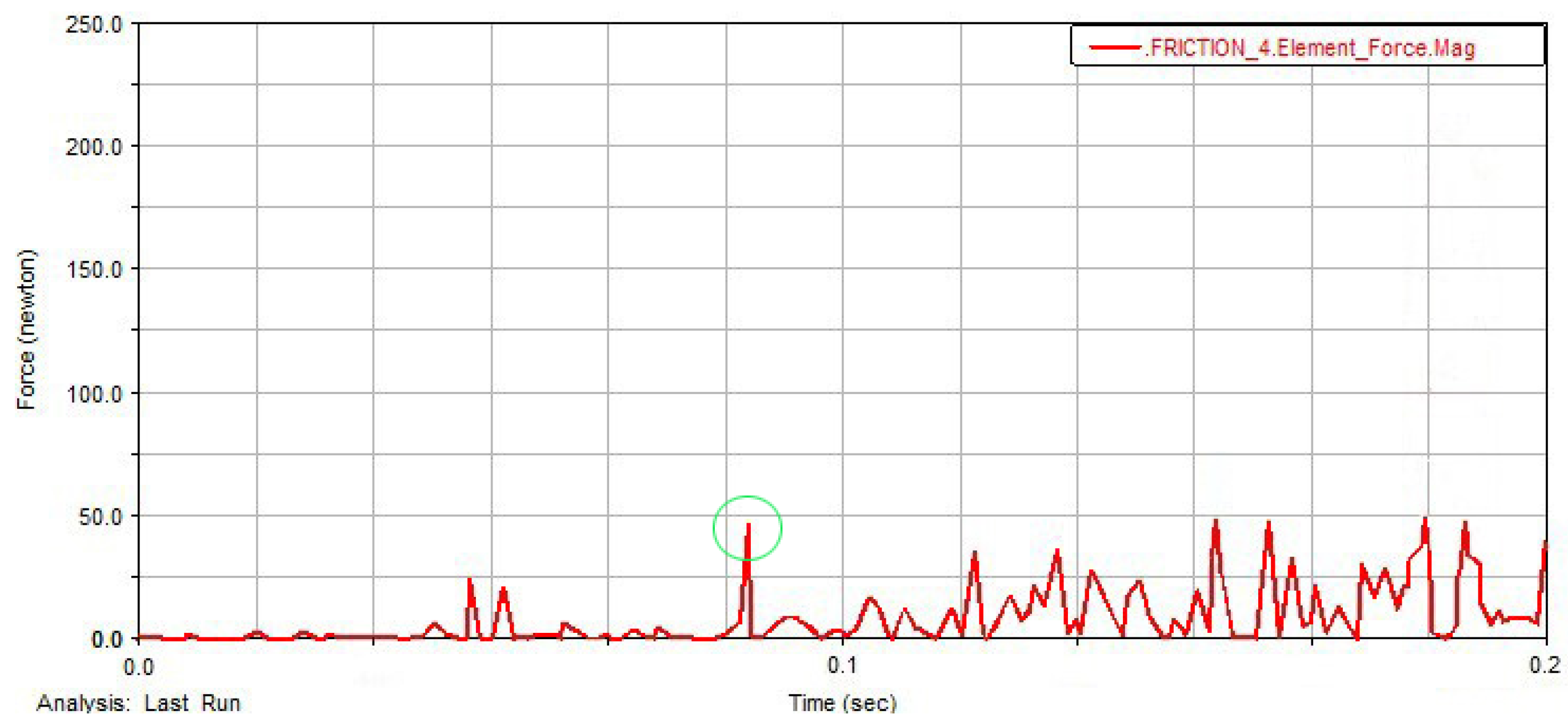
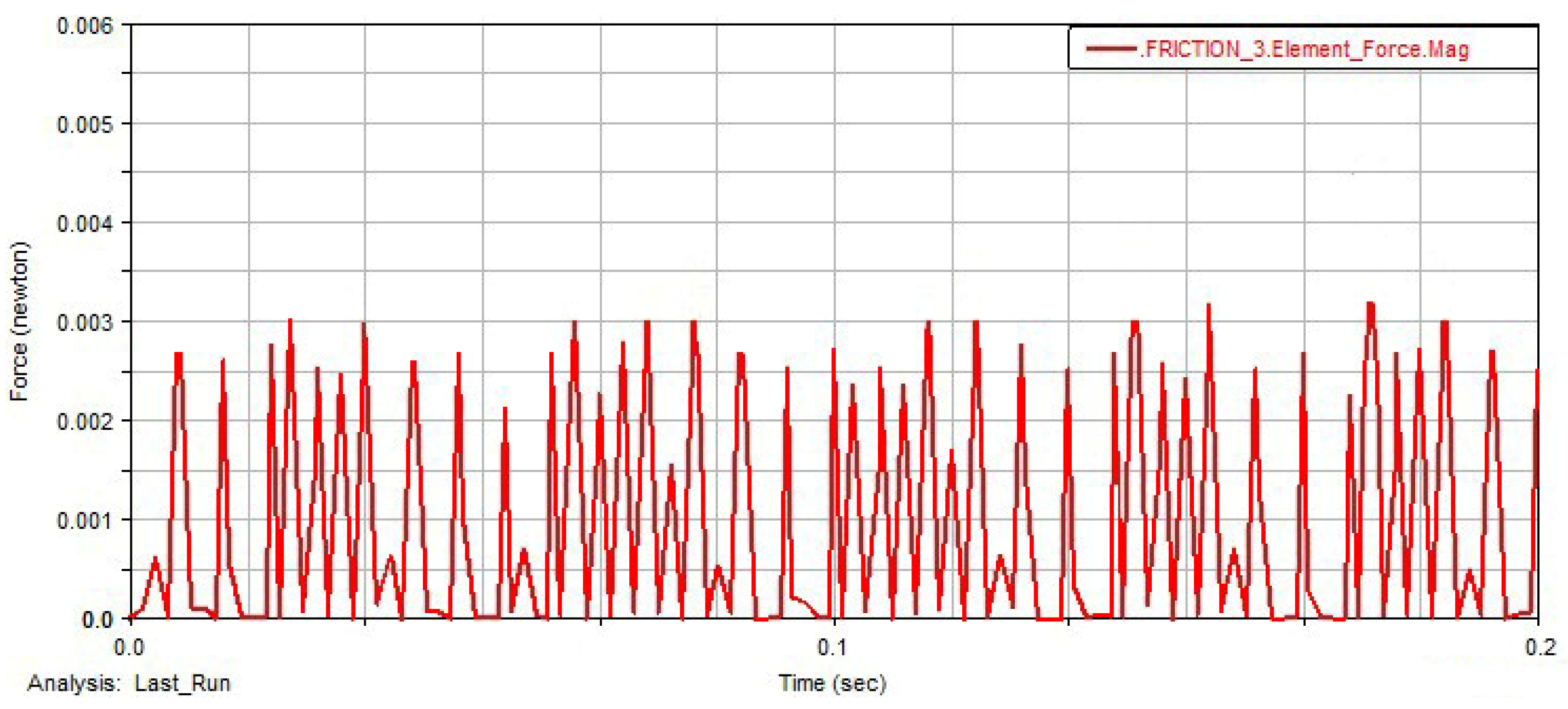
- Friction curves between the slider and rotor slider slot before and after optimizing the stator cavity length and short radius ratio.
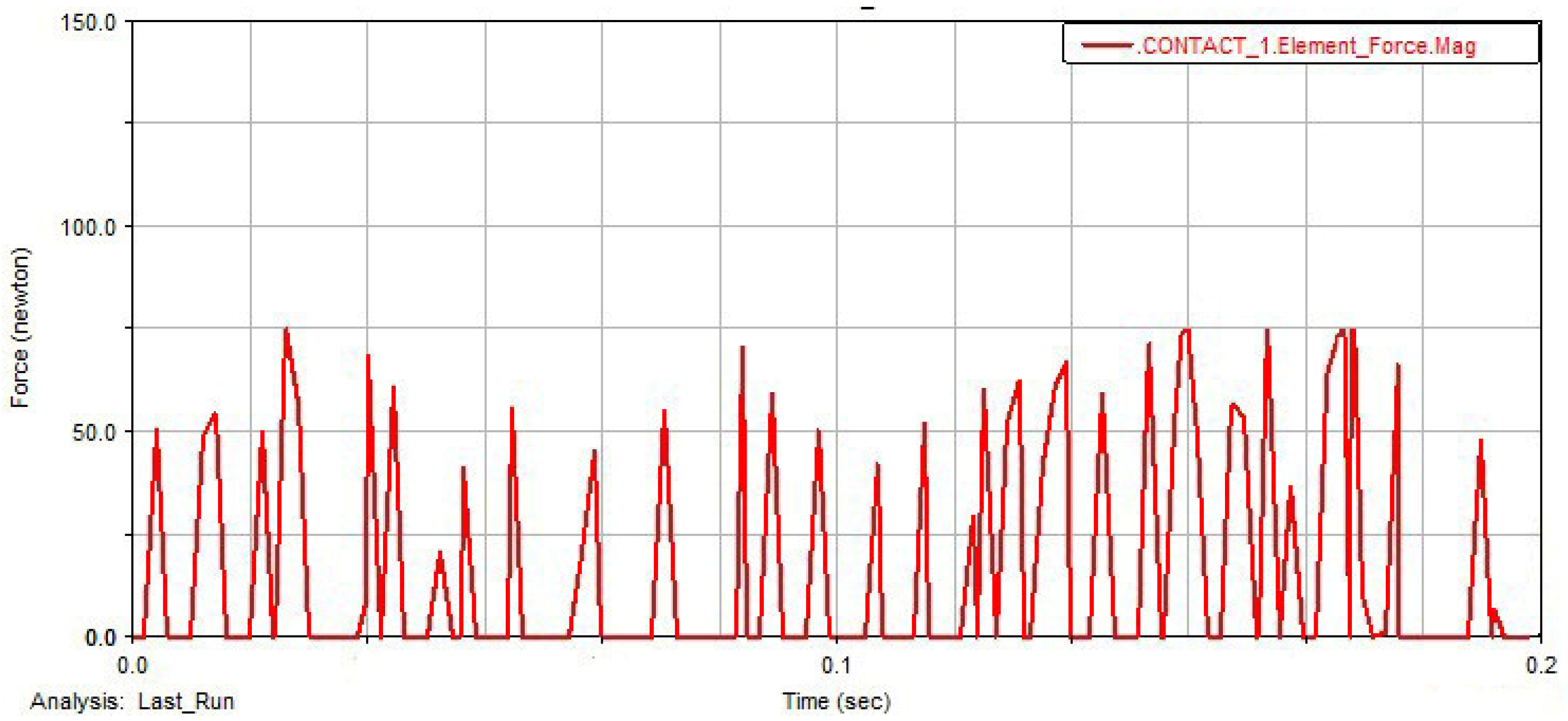
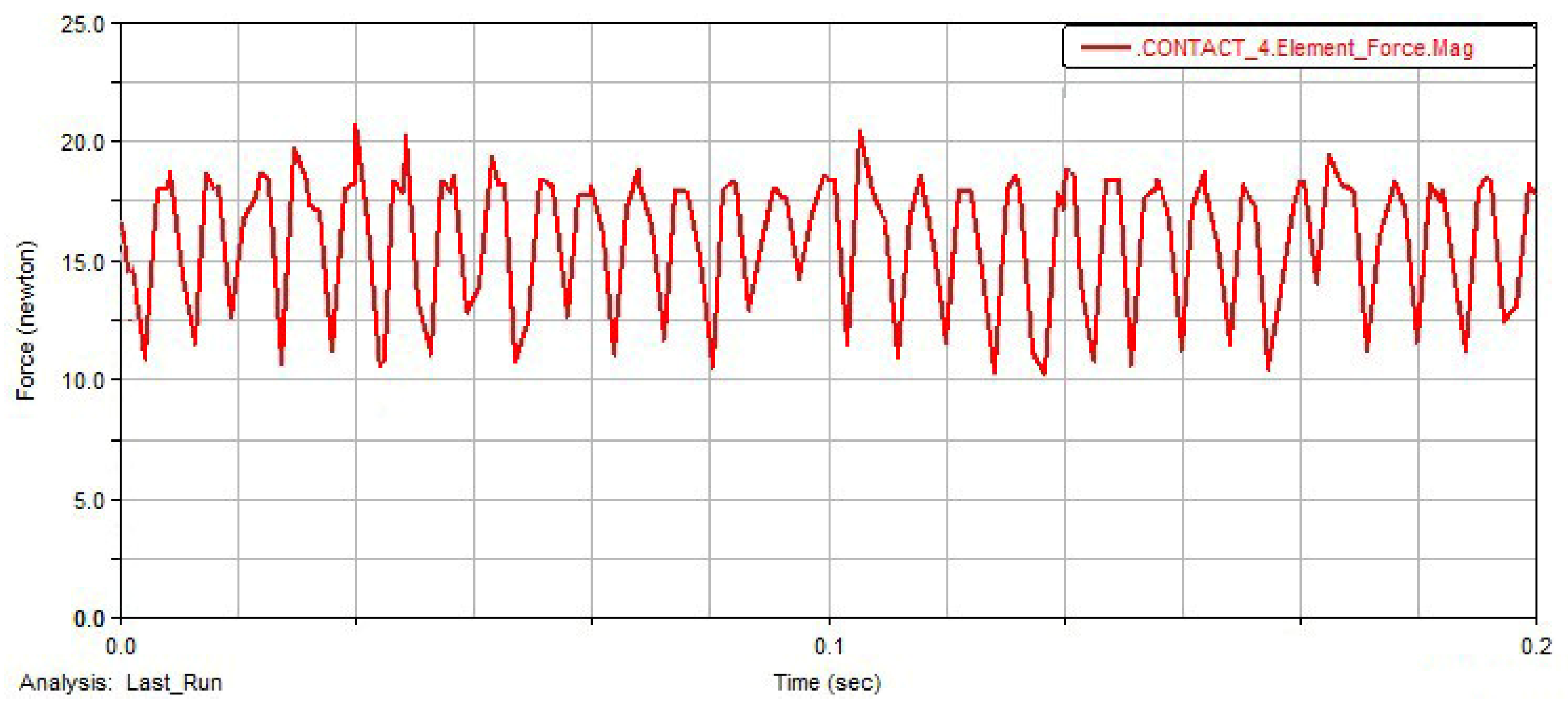
- (4)
- Slider–stator contact force curve before and after optimizing the stator cavity length to short radius ratio.
5. Conclusions
- The explicit expression of the blade contact angle as a function of the blade rotation angle was obtained by fitting the values of the sampling points. The analysis showed that the blade contact angle was maximum in the middle of the transition curve and that the Gaussian approximation method had a good approximation effect.
- The optimization model of the long–short radius ratio using an intelligent particle swarm algorithm. According to the force balance equation, the expression of the sliding friction between the blade and the stator was derived. To minimize the sliding friction force on the edge, the optimized solution of the long–short radius ratio of the inner cavity of the stator was calculated.
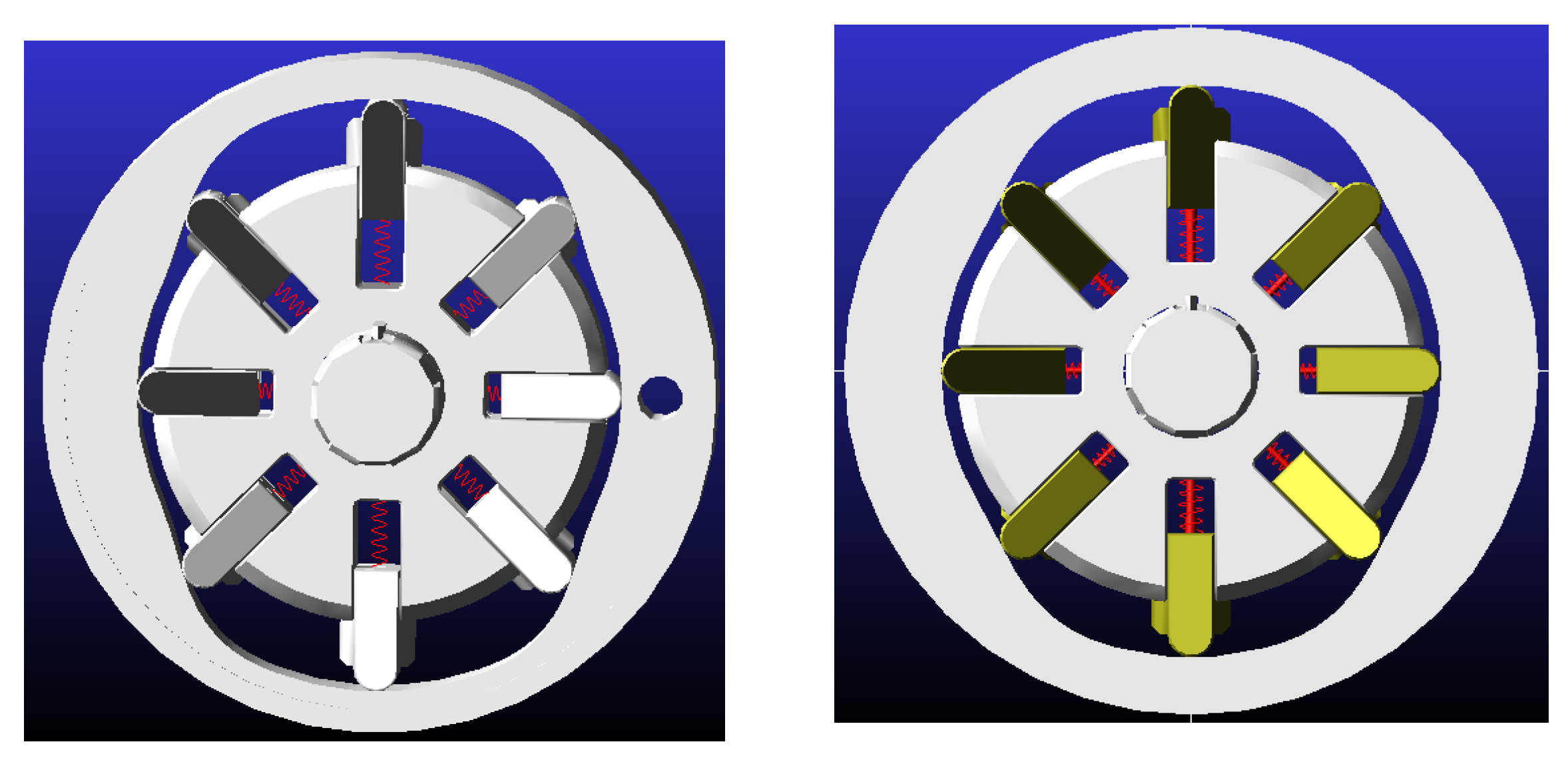
- The dynamics of the vane pump was simulated using Adams separately, and the main shaft torque, vane acceleration, vane and rotor friction, and vane and stator contact force before and after optimization were compared and analyzed. The results showed that the optimized stator performance was better.
Author Contributions
Funding
Institutional Review Board Statement
Informed Consent Statement
Conflicts of Interest
Abbreviations
| Fi | Centrifugal force |
| Ft | Spring force |
| Fm | Inertia force |
| Fk | Coe-type inertia force |
| Fη | Viscous friction force |
| Fn1, Fn2 | Contact reaction force of the rotor |
| mv | the rotating blade center mass |
| ω | the spindle angular velocity |
| R | the stator internal cavity large arc radius |
| r | the stator internal cavity small arc radius |
| ρ(θ) | the blade vector diameter |
| k | the spring stiffness coefficient |
| μ | the spring free length |
| m | the blade mass |
| n | the spindle speed |
| Ff | Friction force between the stator cavity and the stator |
| λc | the distance between the vane center of mass and the stator inner cavity |
| a(θ) | the radial acceleration of the blade in the transition curve section |
| L | the blade length |
| α | the pressure angle formed by the blade and the stator cavity surface |
| ƒ | the friction coefficient |
| V(θ) | the radial velocity of the blade in the transition curve section |
| η | the oil viscosity |
| Ab | the actual contact area between the bottom of the blade and the oil fluid according to the design size of the blade |
| Avs | the actual contact area between the blade and the endplate |
| Avr1 | the actual contact area between the blade and the rotor in the sizeable circular arc section |
| Avr2 | the actual contact area between the blade and the rotor in the small circular arc section |
| Avr | the actual contact area between the blade and the rotor in the stator transition curve section |
| hvr | the clearance between the blade and the rotor |
| hvs | the clearance between the blade and the endplate |
| L1 | the length of the blade extending outside the rotor slot |
| ξ | the coefficient of the contact reaction force of the edge by the rotor on the edge |
| Fp1, Fp2, Fp3, Fp4, Fp5 | Hydraulic pressure |
Appendix A


- (1)
- Material mechanics analysis of slide section

- (2)
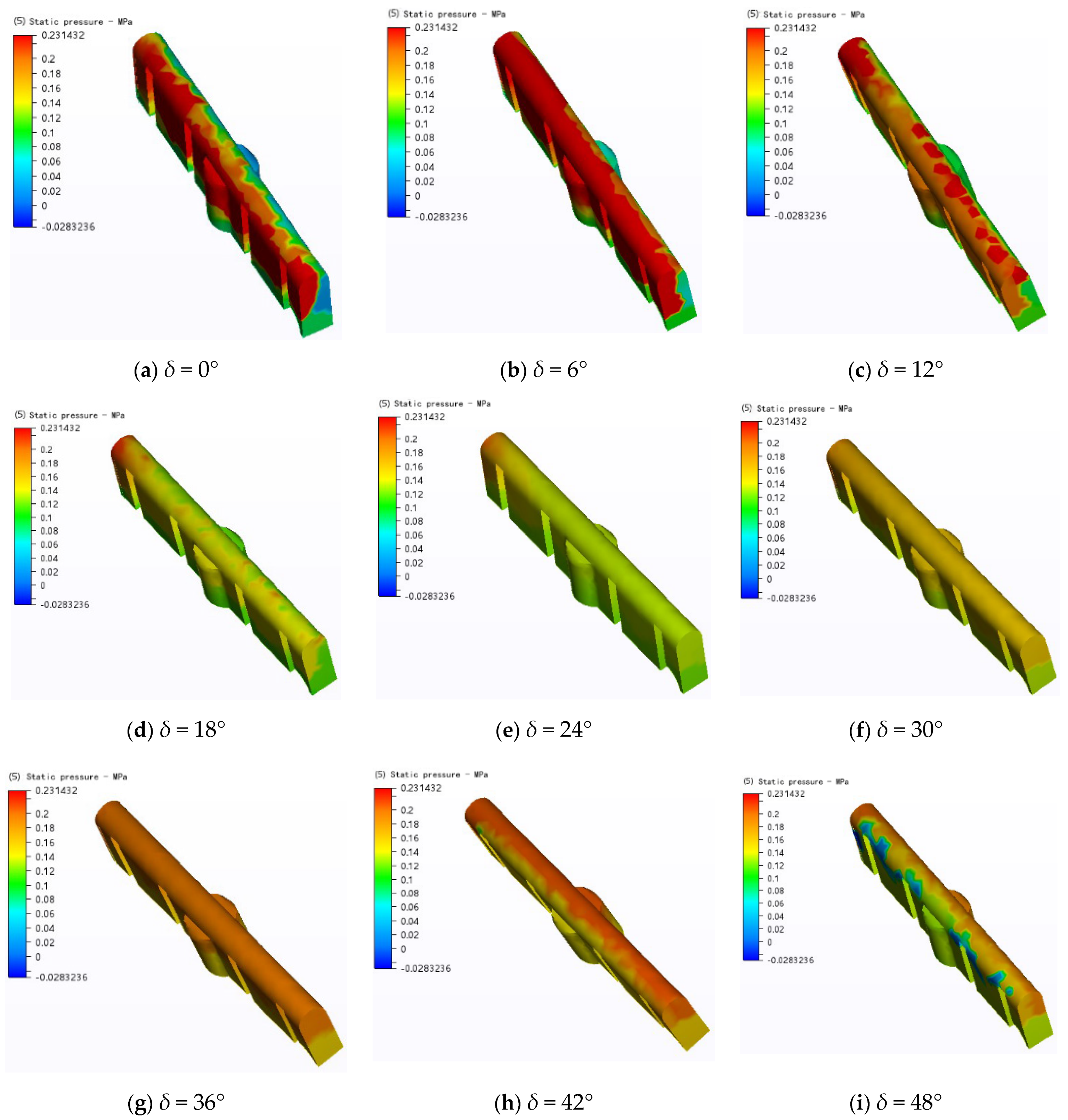
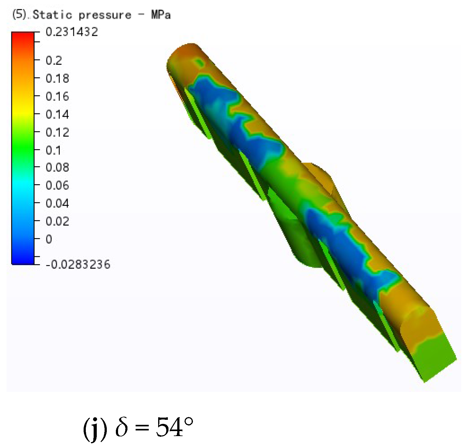
- Suction chamber slider fluid pressure analysis.

(kN) | (kN) | q (kN) | (mm) | (kN) | (kN) | (mm) | (kN) | (kN) | (mm) | (kN) | |
| 0° | 207 | 670.68 | 198 | 4.710 | 466.29 | 28 | 6.48 | 90.72 | 147 | 4.71 | 346.18 |
| 6° | 260 | 842.4 | 312 | 5.024 | 783.74 | 96 | 6.48 | 311.04 | 185 | 4.39 | 406.63 |
| 12° | 250 | 807.5 | 276 | 5.432 | 749.64 | 99 | 6.46 | 319.77 | 210 | 3.98 | 418.71 |
| 18° | 197 | 602.82 | 175.5 | 6.411 | 562.56 | 118 | 6.12 | 361.08 | 145 | 3.01 | 218.22 |
| 24° | 162 | 413.1 | 178.5 | 7.049 | 629.15 | 132 | 5.10 | 336.6 | 245 | 2.37 | 290.41 |
| 30° | 187 | 328.18 | 177 | 7.130 | 631.27 | 169 | 3.51 | 296.59 | 171 | 2.28 | 195.52 |
| 36° | 197 | 181.24 | 198 | 6.421 | 635.70 | 197 | 1.84 | 181.24 | 198 | 2.99 | 296.87 |
| 42° | 204 | 54.06 | 188 | 5.453 | 512.59 | 206 | 0.53 | 54.59 | 199.5 | 1.32 | 131.86 |
| 48° | 188 | 21.62 | 108 | 7.693 | 415.42 | 198 | 0.23 | 22.77 | 171 | 1.72 | 147.65 |
| 54° | 134 | 33.5 | 112 | 4.720 | 264.34 | 189 | 0.50 | 47.25 | 103 | 4.69 | 242.02 |
Appendix B

References
- Ma, W.C. Research status of high-pressure vane pump and its outlook. Fluid Drive Control 2006, 6, 1–6. [Google Scholar]
- Liu, J.G. Development of double-acting variable vane pump. J. Yanshan Univ. 2002, 3, 276–279. [Google Scholar]
- Jing, Y. Sliding vane pump features and development trend. China Storage Transp. 2008, 12, 116–117. [Google Scholar]
- Huang, S.B. Innovative Design and Simulation for a Novel Vane Pump. In Proceedings of the International Conference on Mechatronics and Materials Processing, Guangzhou, China, 18–20 November 2011; pp. 354–359. [Google Scholar]
- Karpenko, M.; Prentkovskis, O.; Šukevičius, Š. Research on high-pressure hose with repairing fitting and influence on energy parameter of the hydraulic drive. Eksploat. I Niezawodn. Maint. Reliab. 2022, 24, 25–32. [Google Scholar] [CrossRef]
- Stosiak, M. Ways of reducing the impact of mechanical vibrations on hydraulic valves. Arch. Civ. Mech. Eng. 2015, 15, 392–400. [Google Scholar] [CrossRef]
- Bai, J.J.; Xu, M.M. Research Status and Development Trend of Vane Pump. In Proceedings of the International Conference on Mechatronics Engineering and Computing Technology, Shanghai, China, 9–10 April 2014; pp. 1143–1146. [Google Scholar]
- Yoshida, Y.; Tsujimoto, Y.; Kawakami, T.; Sakatani, T. Unbalance hydraulic forces caused by geometrical manufacturing deviations of centrifugal impellers. J. Fluids Eng. 1998, 120, 531. [Google Scholar] [CrossRef]
- Ravindra, B.; Appasaheb, K. Prediction of flow-induced vibration due to impeller hydraulic unbalance in vertical turbine pumps using one-way fluid-structure interaction. J. Vib. Eng. Technol. 2019, 8, 417–430. [Google Scholar]
- Li, G.P.; Chen, E.Y.; Yang, A.L.; Xie, Z.B.; Zhao, G.P. Effect of Guide Vanes on Flow and Vibroacoustic in an Axial-Flow Pump. Math. Probl. Eng. 2018, 2018, 3095890. [Google Scholar] [CrossRef]
- Christopher, S.; Kumaraswamy, S. Identification of Critical Net Positive Suction Head Form Noise and Vibration in a Radial Flow Pump for Different Leading Edge Profiles of the Vane. J. Fluids Eng. Trans. ASME 2013, 135, 121301. [Google Scholar] [CrossRef]
- Zhou, W.J.; Cao, Y.H.; Zhang, N.; Gao, B. A novel axial vibration model of multistage pump rotor system with dynamic force of balance disc. J. Vib. Eng. Technol. 2020, 8, 673–683. [Google Scholar] [CrossRef]
- Zhang, L.J.; Wang, S.; Yin, G.J.; Guan, C.N. Fluid-structure interaction analysis of fluid pressure pulsation and structural vibration features in a vertical axial pump. Adv. Mech. Eng. 2019, 11, 1687814019828585. [Google Scholar] [CrossRef]
- Liu, H.L.; Cheng, Z.M.; Ge, Z.P. Collaborative improvement of efficiency and noise of bionic bane centrifugal pump based on multi-objective optimization. Adv. Mech. Eng. 2021, 13, 1687814021994976. [Google Scholar] [CrossRef]
- Si, Q.R.; Wang, B.B.; Yuan, J.P. Numerical and Experimental Investigation on Radiated Noise Characteristics of the Multistage Centrifugal Pump. Processes 2019, 7, 793. [Google Scholar] [CrossRef]
- Cheng, Y.Q.; Wang, X.H.; Chai, H. The Theoretical Performance Analysis and Numerical Simulation of the Cylindrical Vane Pump. Arab. J. Sci. Eng. 2021, 46, 2947–2961. [Google Scholar] [CrossRef]
- Liu, L.; Ding, C.; Wang, P.F. Design and Optimization of the Transition Curve in the Novel Profiled Chamber Metering Pump. J. Multi-Body Dyn. 2020, 234, 435–446. [Google Scholar] [CrossRef]
- Fan, J.; Wang, Z.R. Calculation and analysis of single-acting vane pump stator radial fluid pressure for high-powered remote water supply fire truck water collection system. Fire Technol. Prod. Inf. 2013, 11, 47–50. [Google Scholar]
- Cho, I.S. Behavioral characteristics of the vane of a hydraulic vane pump for power steering systems. J. Mech. Sci. Technol. 2015, 29, 4483–4489. [Google Scholar] [CrossRef]
- Lei, H.; Hu, H.J.; Lu, Y. A dynamic analysis on the transition curve of profiled chamber metering pump. J. Dyn. Syst. Meas. Control 2016, 138, 071003. [Google Scholar] [CrossRef]
- Gao, P. Application of Matlab’s CFtool toolbox to flotation tailings ash and image grayness curve fitting. Coal Process. Technol. 2015, 1, 67–70. [Google Scholar]
- Hou, Z.R.; Lu, Z.S. MATLAB-based particle swarm optimization algorithm and its application. Comput. Simul. 2003, 10, 68–70. [Google Scholar]
- Wang, L.J.; Jiang, S.F.; Xu, F.X. Analysis of particle swarm algorithms and their covariates. J. Qiqihar Univ. 2019, 35, 14–17. [Google Scholar]


| Ab (mm2) | Avs (mm2) | Avr1 (mm2) | Avr2 (mm2) | η (mm2/s) | hvr (mm) | hvs (mm) |
|---|---|---|---|---|---|---|
| 340.58 | 80.03 | 423.54 | 910 | 30 | 0.03 | 0.30 |
| a | ω (rad/s) | ƒ | α | r (mm) | R (mm) | R/r (R ≠ r) |
|---|---|---|---|---|---|---|
| 50° | 100 | 0.13 | [0, 90°] | [32, 34] | [32, 40] | (1, 1.2603] |
Publisher’s Note: MDPI stays neutral with regard to jurisdictional claims in published maps and institutional affiliations. |
© 2022 by the authors. Licensee MDPI, Basel, Switzerland. This article is an open access article distributed under the terms and conditions of the Creative Commons Attribution (CC BY) license (https://creativecommons.org/licenses/by/4.0/).
Share and Cite
Sun, Y.; Xue, D.; Liu, S.; Wu, J.; Bai, X. Stator Curvature Optimization and Analysis of Axial Hydraulic Vane Pumps. Energies 2022, 15, 6229. https://doi.org/10.3390/en15176229
Sun Y, Xue D, Liu S, Wu J, Bai X. Stator Curvature Optimization and Analysis of Axial Hydraulic Vane Pumps. Energies. 2022; 15(17):6229. https://doi.org/10.3390/en15176229
Chicago/Turabian StyleSun, Yongguo, Dong Xue, Shisheng Liu, Jinghang Wu, and Xingyu Bai. 2022. "Stator Curvature Optimization and Analysis of Axial Hydraulic Vane Pumps" Energies 15, no. 17: 6229. https://doi.org/10.3390/en15176229