Long-Term Planning of Electrical Distribution Grids: How Load Uncertainty and Flexibility Affect the Investment Timing

Abstract

Due to the rise of smart grids, new players and services are emerging and can have an impact on the decision-making process in distribution networks, which, over the past decades, were only driven by linear demand growth with a low level of uncertainties. Nowadays, the evolution of distribution networks and investment decisions (conductors and transformers) can no longer be based solely on deterministic assumptions of load evolution since there is a high level of uncertainties related to the development of electrical loads such as electric vehicles. In this paper, we focus on the uncertainty of the peak power, key elements for triggering an investment, and the flexibility to choose between different topologies of electric networks. To solve this problem, we apply a real option approach and provide an analytical model with closed-form solutions that allows a full treatment of the dynamic aspects of the decision to reconsider the topology of the network. Moreover, through a comparative statics analysis, we infer the sensitivity of the option value to modify the network with respect to the volatility of the peak power, the associated investment cost or other types of costs of power losses, the growth rate, or the discount rate.

1. Introduction

The development of transmission and distribution networks requires large investments mainly driven by the increase in demand and the improvement and maintenance of the quality of service. These investments should fulfill important technical requirements such as ensuring the reliability, efficiency, quality, and uninterrupted supply of power. These goals are considered in each step of the investment process, as shown in Figure 1.

Figure 1. Stages of investment studies. Source: own elaboration adapted from [1].

Figure 1. Stages of investment studies. Source: own elaboration adapted from [1].

More particularly, the DSOs (distribution system operator) strike to achieve the least cost objective function through a greater optimization of electrical grid planning and minimization of total costs of serving the demand. Besides other types of costs, including the investment costs, a part of the objective function is represented by those associated with additional technical (power losses, imbalances, etc.) and non-technical losses (thefts, metering errors, etc.), which are determined by the load variation (In European Union countries the annual electricity losses are in average between 2% and 12% [2]). These losses are usually estimated by using the maximum yearly load [1]. Classically, the DSOs consider a deterministic growth rate of maximum load for the coming years and base their investment strategy on it. However, different ongoing and upcoming changes in institutional, economic, societal, and technological contexts bring significant uncertainties in the load evolution and impose operational and development constraints on the electric distribution network.

In this context, our paper criticizes whether investment decisions in distribution networks (conductors and transformers) can still be based solely on deterministic assumptions of load evolution. It does so by conducting a real options analysis. This approach has been widely used to evaluate energy projects under uncertainty [3]. We argue that it makes it especially well suited to evaluate the optimality of the decision to undertake additional investments related, for instance, to the design of the grid under uncertain evolutions of the theoretical maximum power.

The contributions of our paper are three-fold. First, from the theoretical point of view, it complements existing studies on long-term planning and optimization of distribution networks by using a dynamic programming approach [4] and considering the uncertain evolution of the electrical load in a model with closed-form solutions. Most previous studies [5,6,7,8] use linear programming under constraints or Monte Carlo simulations. To our knowledge, this is the first attempt to assess the uncertainty of the maximum power in an analytical model with quadratic form within a continuous time framework, which in turn allows a full treatment of the dynamic aspects of the decision to invest. Second, our paper contributes to the real options valuation approach by considering a quadratic variation of the load [9]. This feature, undoubtedly, adds complexity to the analytical development of the model. Third, from the practical point of view, our aim is to propose a general decision-making tool that the DSOs can use in order to account for flexibility in uncertain environments and obtain the optimal strategy for long-term planning. Compared to current practices based mainly on Monte Carlo simulations specific to given network topology and technical constraints, our analytical solution can be modified in order to incorporate the conditions of any topology of the electrical grid by adjusting the technical and economic parameters.

More precisely, we focus on the timing flexibility to choose between different topologies of electric networks under the uncertain evolution of the load. If the maximum power is sufficiently important, a DSO may decide to change the initial topology with an alternative one. Because the DSO is interested in optimizing its power loss costs, the level of maximum power determines its willingness to undertake the reinforcement cost associated with the increase in lines. Therefore, we derive a rule for switching between different electrical grid topologies, and we find an analytical expression of the optimal level of the maximum power. Not surprisingly, the threshold of the peak power for which it is interesting to reinforce the network is higher than the one in conventional cases. When new information arrives over time, the DSO has the flexibility to use it and thus choose the optimal timing. If there is significant uncertainty about future maximum yearly load, the real options embedded in incremental investment programs (such as small grid upgrades) or other approaches that defer grid investment (such as the use of grid alternatives) can be valuable, potentially outweighing the economies of scale advantage of large upgrades. Moreover, through a comparative static analysis, we infer the sensitivity of the option value to reconfigure the network with respect to the volatility of the peak power, the associated investment cost or other types of costs of power losses, the growth rate, or the discount rate.

In addition to this introduction, the paper is organized as follows. Section 2 presents the methodological context and the literature review, while Section 3 covers the assumptions, the development of the model, and the closed-form solutions. Section 4 discusses the results through a numerical illustration and comparative statics analysis. Section 5 brings in some policy implications of our modeling framework and concludes the paper.

2. Methodology and Related Literature

The assessment of investment decisions in distribution networks was traditionally tackled with a wide range of models, from deterministic to probabilistic frameworks [10,11,12]. Given the technical constraints and the specificity of each network, most of these approaches are hybrid, with an unclear frontier between them. This makes it difficult to compare them and emphasize the best one (the usefulness in terms of policy implications of such a comparative study is undeniable but lies outside the limited scope of our present paper). Nevertheless, commonly used methods are based on optimization through mixed-integer linear programming and probabilistic approaches such as analytical, Monte Carlo, or fuzzy logic [7,13,14]. One limit of these methods is related to their high dependency on data and construction of scenario simulations that obstructs their general use. In addition, despite their consideration, they do not explicitly capture the positive effect of uncertainties in the decision-making process. Alternatively, a well-known decision tool from economic theory recognizes that the arrival of new information through time adds value to an investment project, i.e., creates an option [4,15,16]. The concept of option value can complement traditional methods and consider adjustments to the parameters of a project in an uncertain environment. More particularly, the intuition underlying the real options concept is straightforward: there may be a value associated with the option to postpone a decision until some uncertainty about the variables that influence it is resolved. Depending on whether the circumstances are favorable or not, the decision maker has the right but not the obligation to perform an action or to take a decision. By readily acknowledging that one can adjust the strategy to the prevailing circumstances, the consideration of the option value in the evaluation may be a source of new opportunities and/or mitigate actual or future losses. Because grid investment programs are characterized by high sunk costs and uncertain benefits, the flexibility in the decision-making process is likely to be valuable.

Since the rise in renewables investments and the deregulation of energy markets, the electrical system has seen a sharp increase in uncertainty, which has induced a significant increase in the use of real options for investment valuation, whether it is in production, infrastructure, or R&D programs. However, most of the effort made pertains to investments in transmission network reinforcement or expansion and generation investment assessment. Among these, we have identified the works [17,18,19,20,21] that highlight the flexibility that real options analysis provides in the context of transmission power systems through different types of investment decisions, simulation methods, and optimal outcomes.

Several studies [22,23,24,25] explore real options in conjunction with investments in electricity distribution networks. Most of these papers consider discrete time frameworks and linear cost functions to assess various types of options associated with the investment decision: abandon or relocate distributed generation (DG) to add flexibility in distribution network expansion planning, expand with extra capacity, reinforce or use of demand side response, defer the network investment due to energy storage systems (ESS). The decision to invest is guided by the uncertain load growth, which is assessed through Monte Carlo simulations or stochastic processes such as GBM (geometric Brownian motion).

Our goal is to contribute to the existent literature on the uncertain evolution of maximum yearly power by using dynamic programming to obtain closed-form solutions in a continuous time framework. Compared to previous works, we consider a polynomial form of cost functions with a quadratic yearly variation of maximum load in the case of power losses and linear evolution for power outages and energy not supplied associated costs. The advantage of this approach is its increased traceability, its guarantee to reach faster an optimal solution, and detailed characterization of the optimal strategy to switch between two types of electric grid topologies.

3. The Model

This section develops the model based on the technical characteristics of the power system and uses the maximum consumption power as a source of uncertainty. The DSO has the opportunity to invest in network reinforcement in order to reduce costs, as well as to avoid constraints rising from a mismatch between the load and the operational limit of the equipment. Using dynamic programming and real options theory, we determine the optimal threshold that triggers investment decisions when load uncertainty is considered.

3.1. Problem Statement

In order to maintain the high standards of electrification imposed by regulators, DSOs have to invest large capital either to ensure delivery of the required power while increasing and maintaining its quality or to optimize the economic performance of the system. As an example, let us consider a DSO that has the option to make new investments in order to obtain an economical and technical optimization of the electric network topology. He can do so by migrating from an initial topology with two feeders, presented in the left part of Figure 2, to a more cost-effective one with three feeders. This migration entails a reduction in the circulating currents in the power lines and an increase in the availability of the system. These improvements directly contribute to the reduction in the operational expenditures but come at a high capital cost resulting from the need to invest in new infrastructure to support this re-distribution of the loads [26]. Moreover, in this case, study, the proposed system is a medium voltage (MV) network that consists of an HV/MV substation, MV power lines, MV customers, and MV/LV substations.

Figure 2. Network evolution between today and year T [27].

Figure 2. Network evolution between today and year T [27].

After the optimization of the network from the technical point of view, the DSO seeks to optimize the sizing of investment (different cable sections retained by DSO, the unit power of transformers, etc.) and the level of electrical losses. At this stage, given the magnitude of the capital investment needed to expand the network, the DSO tries to determine whether the savings made on the OPEX justify the investment. In addition, the DSO determines the optimal investment timing for which the returns on investment are the greatest. This technical-economic optimization is currently carried out in a discrete time framework using DCF (discounted cash-flow) as described in [28] (for details, see Appendix F). Our work focuses on this layer of economic optimization by taking into account uncertainties inherent in the evolution of the load.

3.2. Main Assumptions

This part explains the main technical and economic assumptions that characterize the parameters of the decision problem for reinforcing the network.

Table 1. System nomenclature.

Technical Parameters		Unit
t	Time index	year
$t_u$	Subtime index of t	hour
T	Time horizon	Year
k	k = {wr, r} wr: without reinforcement, r: with reinforcement	-
$P_{max}\left(t\right)$	Maximum active power of the HV/MV substation at time t	W
i	Feeder index
$I_{max,i,k}\left(t\right)$	Module of the maximum current at time t through the feeder i for strategy k	A
$R_{i,k}$	Linear resistance of feeder i for strategy k	Ω/km
$l_{i,k}$	Length of feeder i for strategy k	km
$L_{max,i,k}\left(t\right)$	Power losses in feeder i for strategy k at time t	W
U	Nominal phase-to-phase voltage of the MV network	V
$S_{max,i,k}\left(t\right)$	Maximum apparent power of the customer connected to feeder i for strategy k at time t	VA
$P_{max,i,k}\left(t\right)$	Maximum active power of the customer connected to feeder i for strategy k at time t	W
$\mathrm{S}(t_u$)	Apparent power of the HV/MV substation at time $t_u$	VA
$\mathrm{P}(t_u$)	Active power of the HV/MV substation at time $t_u$	W
$P_{average}\left(t\right)$	Average power of the HV/MV substation at time t	W
μ	Growth rate of maximum power	%
$\sigma$	Volatility	%
${\xi }_{i,k}$	Constant depending on the conductor type, length, and voltage for feeder i, strategy k	Ω/V2
${\eta }_{i,k}$	Power ratio of feeder i for strategy k	-
${\tau }_u$$, {\tau }_o$	Respectively underground and overhead feeder failure rate	Failure/year/100 km
$l_{u,i,k}$$, l_{o,i,k}$	Respectively underground and overhead length of feeder i for strategy k	km
$H_{max}$	Equivalent maximum power runtime	hour
$T_{out,i,k}$	Average power outage duration for feeder i for strategy k	hour
$N_k$	Number of MV feeders of the HV/MV transformer for strategy k	-
$NP{V}_k$	Net present value of the total discount cost for strategy k	€
$\cos \phi$	Power factor of the customer (assumed constant)	-
Economic Parameters		Unit
$C_{cable}$	Cost of underground line (including the trench)	€/km
$C_{line}$	Cost of overhead line	€/km
$C_{losses}$	Cost of peak power losses	€/W
$C_{END}$	Cost of energy not supplied	€/Wh
$C_{out}$	Cost of power outage	€/W
$\delta$	Discount rate	%
$C_{total losses,k}$	Annual cost of power losses for strategy k	€
$C_{total out,k}$	Annual cost of power cut due to outages	€
$C_{total END,k}$	Annual cost of the energy not delivered to the customers due to outages	€
$OPE{X}_k$	Operational expenditure of strategy k	€

presents the variables and system characteristics.

Given the nonlinearity of power flows, the absence of smart metering, and the presence of multiple uncertain variables, several assumptions and simplifications were made. These assumptions help render our model close to the one already in use by some DSOs while allowing the seamless introduction of uncertainty into the equations.

Assumption 1.

Figure 3 shows the connection model between the MV/LV nodes, modeled as customers, and the source substation, modeled as the transformer.

The operation of the distribution network may involve technical and non-technical losses, each of them coming with associated costs. Given the difficulty of estimating the non-technical losses (as stated by Chauhan and Rajvanshi [29], technical losses can easily be calculated using load flow computation, while non-technical losses require highly complex estimation methods to be computed), we further focus on the technical ones. These losses, also called power losses, are caused by the resistivity of the cable’s material to transiting current and characterize the transformation of electrical energy into heat. The technical parameters impacting the maximal value of power losses at a given moment t are the feeder linear resistance ($R_{i,k}$) and length ($l_{i,k}$), the power of the customer ($P_{max,i,k}\left(t\right)$), the feeding voltage (U), and the power factor ($\cos \phi$). Thus, the power losses observed in the system at date t are calculated using the following equation (Appendix A):

$$L_{max,i,k}\left(t\right)=\frac{R_{i,k}{l}_{i,k}}{U^2{\cos }^2\phi }\times {\mathsf{\eta }}_{\mathrm{i},\mathrm{k}}{}^2\times P_{max}{\left(\mathrm{t}\right)}^2$$

(1)

were ${\eta }_{i,k}=\frac{P_{max,i,k}\left(0\right)}{P_{max}\left(0\right)}$ is the ratio of the maximum power through each feeder i with the total maximum power of the HV/MV substation for each strategy k. It is considered constant throughout the study period.

Also, a simplification of the average power calculation was made in order to keep the number of stochastic variables at one (Appendix B):

$$P_{average}\left(\mathrm{t}\right)=\frac{H_{max}}{8760} P_{max}\left(\mathrm{t}\right)$$

(2)

$H_{max}$ is considered constant for each feeder, strategy, and throughout the study period, meaning that $\frac{P_{max}\left(t\right)}{P_{average}\left(t\right)}$ remains constant.

Assumption 2.

Conventionally, reinforcement decisions in power systems are based on the maximum power and the load evolution. As shown in Figure 4, the load variation does not follow a regular pattern, and many factors determine and reshape its curve: the number of intermittent decentralized production installations, their coupling to storage means, the number of electric vehicles connected to the network, and the types of charging stations start to have a significant impact on the load evolution [30].

Figure 4. Consumption profiles in France between 2016 and 2020 [31].

Figure 4. Consumption profiles in France between 2016 and 2020 [31].

We follow [17,23,24], and we consider that the normal and smooth variations of the maximum power, $P_{max}$, such as the lights switching, the power consumption of different electrical equipment and appliances are described by the Wiener increment associated with the geometric Brownian motion (GBM) process:

$$d{P}_{max}=\mu P_{max}\left(t\right)dt+\sigma P_{max}\left(t\right)dz$$

(3)

where $dt$ is the time variation and $dz$ the increment of a Wiener process with E [$dz$] = 0 and Var($dz$) = ${ϵ}_{t}dt$, ${ϵ}_t$ is a normally distributed random variable (E [${ϵ}_t$] = 0, Var (${ϵ}_t$) = 1). In this equation, we can clearly see the exponential evolution of the load power ($d{P}_{max}=\mu P_{max }\left(t\right)dt$) corresponding to the DSO models and the uncertainty in its variation ($\sigma P_{max}\left(t\right)dz$). Figure 5 shows a comparison between the stochastic model and the traditional deterministic model, which assumes an annual linear evolution of $P_{max}$.

Assumption 3.

Three types of costs are considered and particularly those associated with power losses, power outages, and energy not supplied. They are described as follows:

$$\begin{gathered} C_{total losses,k}\left(P_{max}\left(t\right)\right)={\displaystyle \sum }_{i=1}^{N_k}{C}_{losses}{\xi }_{i,k}{\eta }_{i,k}^2{P}_{max}{\left(t\right)}^2 \\ with {\xi }_{i,k}=\frac{R_{i,k}{l}_{i,k}}{U^2{cos}^2\phi } \\ {C}_{total out,k}\left(P_{max}\left(t\right)\right)={\displaystyle \sum }_{i=1}^{N_k}{C}_{out}\left({\tau }_o{l}_{o,i,k}+{\tau }_u{l}_{u,i,k}\right){\eta }_{i,k}\frac{H_{max}}{8760}{P}_{max}\left(t\right) \\ {C}_{total END,k}\left(P_{max}\left(t\right)\right)={\displaystyle \sum }_{i=1}^{N_k}{C}_{END}\left({\tau }_o{l}_{o,i,k}+{\tau }_u{l}_{u,i,k}\right){\eta }_{i,k}{T}_{out,i,k}\frac{H_{max}}{8760}{P}_{max}\left(t\right) \end{gathered}$$

(4)

The cost of the losses associated with power outages occurring in the electrical system is calculated based on individual consumer data pertaining to the power cut and the duration of the outage. Normally, these power outages are caused by routine maintenance operations or by circuit trips due to faults occurring in the system (short circuits, damaged infrastructure, etc.) [32]. These costs are modeled using the cost of power that was cut, $C_{total out}$, and the cost of the energy that was not delivered to the customers due to that outage, $C_{total END}$. Risks of failure are summarized using ${\tau }_o$ and ${\tau }_u$ for overhead and underground failure rates, respectively.

Assumption 4.

In addition to operational and maintenance costs, the reinforcement of the grid implies a CAPEX investment concerning the installation of additional equipment to support the extension of the grid, reduce operational costs, increase the quality of service, etc. These investments are considered sunk costs and, in this case, are valued using cable cost, additional transformer feeder cost, and cost of installation (labor, concrete ducts, poles, etc.). In addition, since the change in the topology of the network may take time to be operational, it may involve other costs associated with this delay. For simplicity’s sake, we ignore these time lags in our analysis.

Assumption 5.

The DSO configures the network for the upcoming T years with an expected change in the consumed power that renders the new topology more profitable or adequate, either from a cost or quality of service point of view.

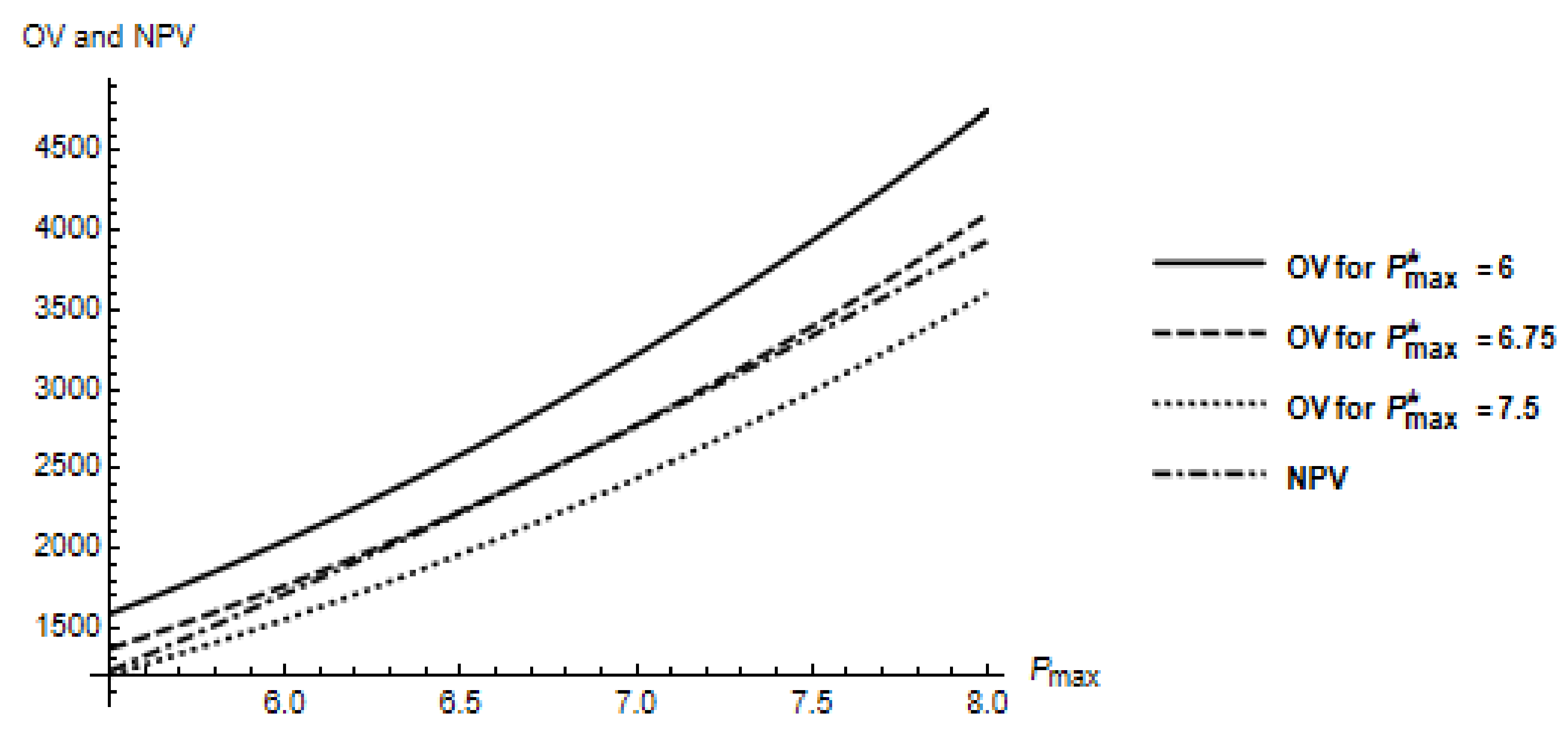
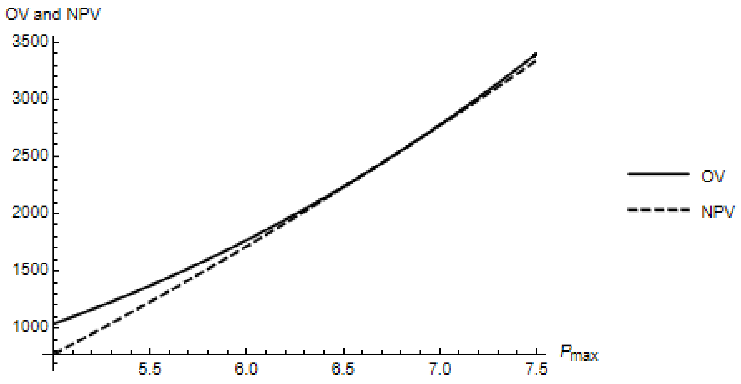
3.3. What Value for the Option to Reinforce the Network?

The long-term planning of electricity distribution networks may include the possibility to change at time t, the number of feeders $\left(N_k\right)$ of the HV/MV transformer for a given strategy k = {wr, r} (“wr” meaning without reinforcement and “r” meaning with reinforcement). Through the decision problem of changing from $N_{wr}\to N_r$, the DSO’s objective is to reduce the expected costs, whether operational or associated with the investment. The expected running costs are the continuous sum of the discounted costs over the studied period and are calculated using Equation (5):

$$OPE{X}_k(P_{max})=E\left[{{\displaystyle \int }}_0^T{e}^{-\delta t}{{\displaystyle \sum }}_{j=1}^3{a}_j{P}_{max}^{{\gamma }_j}\left(t\right)dt|P_{max}\left(0\right)=P_{max}\right]$$

(5)

where $a_j$ are the constants associated with each type of costs, i.e.:

$a_1={{\displaystyle \sum }}_{i=1}^{N_k}{C}_{END}\left({\tau }_o{l}_{o,i,k}+{\tau }_u{l}_{u,i,k}\right){\eta }_{i,k}{T}_{out,i,k}\frac{H_{max}}{8760}; a_2={{\displaystyle \sum }}_{i=1}^{N_k}{C}_{out}\left({\tau }_o{l}_{o,i,k}+{\tau }_u{l}_{u,i,k}\right){\eta }_{i,k}\frac{H_{max}}{8760};a_3={{\displaystyle \sum }}_{i=1}^{N_k}{C}_{losses}{\xi }_{i,k}{\eta }_{i,k}^2;$ and ${\gamma }_j$ are the polynomial exponents with ${\gamma }_1={\gamma }_2=1 \mathrm{and} {\gamma }_3=2$.

We remind that a variable with an initial value at t = 0 of $P_{max}\left(0\right)=P_{max}$ that follows a GBM process has an expected value at a future date t shown in Equation (6) [33]:

$$\mathrm{E}[P_{max}^{{\gamma }_j}\left(t\right)]=P_{max}{e}^{{\gamma }_j(\mu +\frac{{\sigma }^2}{2}({\gamma }_j-1))t}$$

(6)

Considering the expected value of a stochastic polynomial and using the interchange of limiting operators on the sum and integral operators (Fubini’s theorem), the reduced form of Equation (5) can be rewritten as follows:

$$OPE{X}_k(P_{max})={\displaystyle \sum }_{j=1}^3\frac{a_j{P}_{max}{}^{{\gamma }_j}}{\delta -\mu {\gamma }_j-\mu -\frac{{\sigma }^2}{2}({\gamma }_j^2-{\gamma }_j)}\left(1-e^{-\left(\delta -\mu {\gamma }_j-\frac{{\sigma }^2}{2}\left({\gamma }_j^2-{\gamma }_j\right)\right)T}\right)$$

(7)

which has a finite solution if $\frac{\delta }{{\gamma }_j}>\mu +\frac{{\sigma }^2}{2}\left({\gamma }_j-1\right)$ (the assumption that the relative drift of ${\mathsf{\gamma }}_{\mathrm{j}}(\mu +\frac{{\mathsf{\sigma }}^2}{2}({\mathsf{\gamma }}_{\mathrm{j}}-1))$ should be lower than the discount rate is needed in order to ensure the tangency with the NPV. If the condition is not satisfied, waiting would always be optimal, and the reinforcement of the grid should never be undertaken).

The decision maker’s objective at each date t is to minimize the OPEX of the network and is based on the value of maximum power for which the reinforcement decision is optimal.

Decision rule: The decision to reinforce the network from an initial topology (wr) to another one (r) must be taken in order to minimize costs associated with the long-term distribution grid planning. At any date t, the optimal strategy is defined by:

• If $P_{max}<P_{max}^{\ast }$, the DSO decides to continue with the actual configuration of the grid
• If $P_{max}\ge P_{max}^{\ast }$, the DSO takes the decision to reinforce by adding an additional feeder

Likewise, we can write the expected value of the grid distribution planning by taking into account the option to add a new feeder, as follows:

$$V_{wr\to \mathrm{r}}(P_{\max })=\left\{\begin{array}{l}OPE{X}_{\mathrm{wr}}\left(P_{max}\right)-F(P_{max}), if P_{max}<P_{max}^{\ast }\\ OPE{X}_{\mathrm{r}}\left(P_{max}\right)+CAPEX , if P_{max}\ge P_{max}^{\ast }\end{array}\right.$$

(8)

where $CAPEX=C_{cable}{l}_{u,i,r}+C_{line}{l}_{o,i,r}.OPE{X}_{\mathrm{wr}}\left(P_{max}\right)$ and $OPE{X}_{\mathrm{r}}\left(P_{max}\right)$ are the net present values of operational expenditures described in Equation (7) representing the system, respectively, without reinforcement and with reinforcement. $F(P_{max})$ represents the value of the option to reinforce the grid. The DSO is searching to maximize the return from holding the option to reinforce, and consequently, maximizing the option value corresponds to the maximization of the net cost savings from changing the configuration of the grid. The decision maker takes the decision to invest or not at date t in such a way that the option value satisfies:

$$F(P_{max}\left(t\right),t)=Max\left(OPE{X}_{wr}(P_{max}\left(t\right),t\right)-OPE{X}_r(P_{max}\left(t\right),t)-CAPEX\left(t\right),0)$$

(9)

Furthermore, according to the dynamic programming principle, the value of holding the option is equal to the option’s capital appreciation. Using Bellman’s principle, we can write:

$${\mathrm{E}}_{\mathrm{t}}\left[dF(P_{max}\left(t\right),t)\right]=\delta F(P_{max}\left(t\right),t)dt$$

(10)

After applying Itô’s lemma to the differential equation from the right side of Equation (10), the particular solution from Equation (11) is obtained (Appendix C):

$$F\left(P_{max}\right)=\mathrm{A}{P}_{max}^{\beta }$$

(11)

where A is the coefficient of the option value to reinforce the network with a new power line and $\mathsf{\beta }$ is the positive root of the characteristic equation containing the uncertainty parameters: $\frac{1}{2}{\sigma }^2+\left(\mu -\frac{1}{2}{\sigma }^2\right)\beta -\delta =0$.

The optimality of the solution is ensured by the continuity and the smooth pasting conditions from the system of Equation (12). (More detailed explanation of these conditions can be found in Appendix C of chapter 4 in [4]).

$$\begin{gathered} OPE{X}_{\mathrm{wr}}\left(P_{max}^{\ast }\right)-OPE{X}_{\mathrm{r}}\left(P_{max}^{\ast }\right)-\mathrm{CAPEX}=\mathrm{A}{P}_{max}^{\ast }{}^{\beta } \\ \frac{\partial OPE{X}_{\mathrm{wr}}}{\partial P_{max}^{\ast }}\left(P_{max}^{\ast }\right)-\frac{\partial OPE{X}_{\mathrm{r}}}{\partial P_{max}^{\ast }}\left(P_{max}^{\ast }\right)=\beta \mathrm{A}{P}_{max}^{\ast }{}^{\beta -1} \end{gathered}$$

(12)

The value matching condition reflects the fact that, for a given trigger value, the net present value of costs associated with the difference between the OPEX before the reinforcement and the OPEX after reinforcement plus the investment cost should equal the option value of reinforcement. The smooth pasting condition guarantees that the option value can be maximized, and the solution is optimal when the DSO reinforces the grid at $P_{max}^{\ast }.$ Solving the system of these two simultaneous equations leads to a closed-form solution, the threshold $P_{max}^{\ast },$ and the option value coefficient, A.

Proposition. 

The optimal strategy to reinforce the electric grid is characterized by:

 i. 

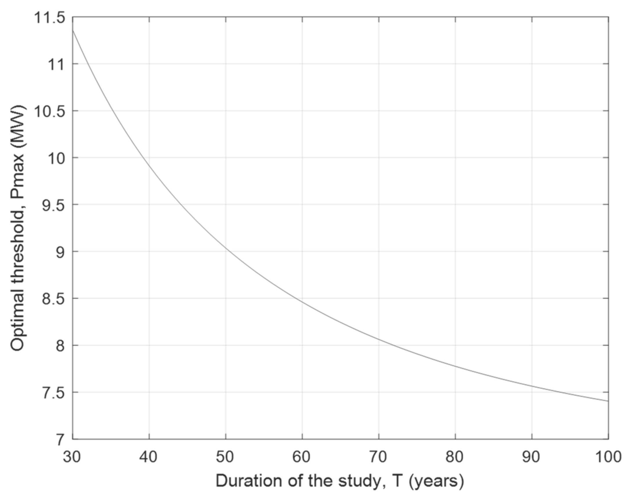
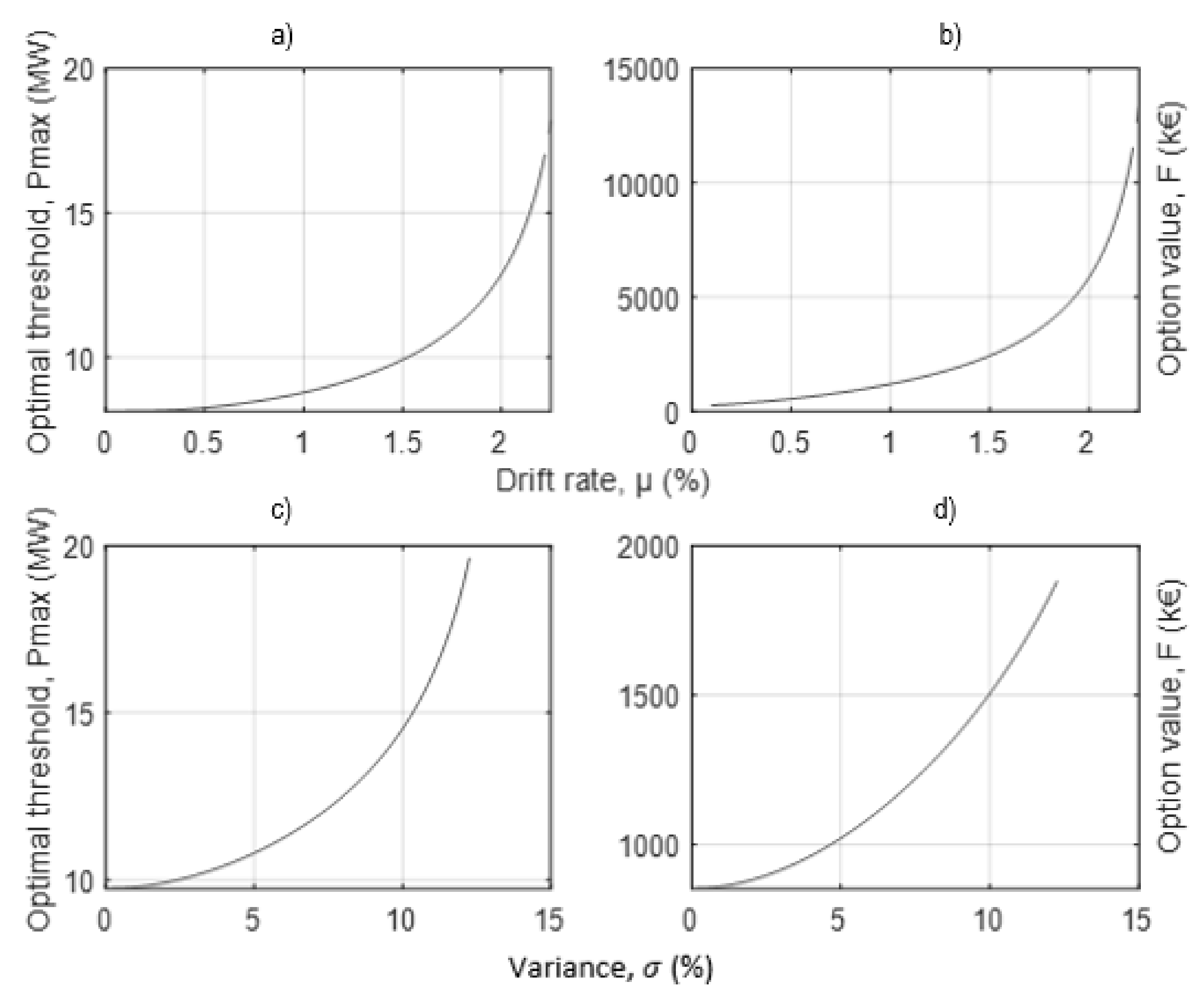
The maximum power for which the reinforcement of the electric distribution grid is optimal is the positive root of the following second-order equation:

$$\left(\beta -2\right)G_{losses}{P}_{max}^{\ast }{}^2+\left(\beta 1\right)\left(G_{END}+G_{out}\right)P_{max}^{\ast }+\beta CAPEX=0$$

(13)

with

$$G_{losses}=C_{losses}\left({\displaystyle \sum }_{i=1}^{N_{\mathrm{wr}}}{\xi }_{i,\mathrm{wr}}{\eta }_{ i,\mathrm{wr}}^2-{\displaystyle \sum }_{i=1}^{N_{\mathrm{r}}}{\xi }_{i,\mathrm{r}}{\eta }_{i,\mathrm{r}}^2\right)\frac{(1-e^{-\left(\delta -2\mu -{\sigma }^2\right)T})}{\delta -2\mu -{\sigma }^2}$$

$$G_{END}=C_{END}\left({\displaystyle \sum }_{i=1}^{N_{\mathrm{wr}}}\left({\tau }_u{l}_{u,\mathrm{i},\mathrm{wr}}+{\tau }_o{l}_{o,\mathrm{i},\mathrm{wr}}\right){\eta }_{i,\mathrm{wr}}{T}_{out,i,\mathrm{wr}}-{\displaystyle \sum }_{i=1}^r\left({\tau }_u{l}_{u,\mathrm{r}}+{\tau }_o{l}_{o,\mathrm{i},\mathrm{r}}\right){\eta }_{i,\mathrm{r}}{T}_{out,i,\mathrm{r}}\right)\frac{H_{max}}{8760}\frac{\left(1-e^{-\left(\delta -\mu \right)T}\right)}{\delta -\mu }$$

$$G_{out}=C_{out}\left({\displaystyle \sum }_{i=1}^{wr}\left({\tau }_u{l}_{u,\mathrm{i},\mathrm{wr}}+{\tau }_o{l}_{o,\mathrm{i},\mathrm{wr}}\right){\eta }_{i,\mathrm{wr}}-{\displaystyle \sum }_{i=1}^{N_{\mathrm{r}}}\left({\tau }_u{l}_{u,\mathrm{i},\mathrm{r}}+{\tau }_o{l}_{o,\mathrm{i},\mathrm{r}}\right){\eta }_{i,\mathrm{r}}\right)\frac{H_{max}}{8760}\frac{\left(1-e^{-\left(\delta -\mu \right)T}\right)}{\delta -\mu }$$

 ii. 

The value of the option to reinforce the network with a new feeder is determined as follows:

$$F\left(P_{max}\right)=\frac{2G_{losses}{P}_{max}^{\ast }{}^2+\left(G_{END}+G_{out}\right)P_{max}^{\ast }}{\beta }{\left(\frac{P_{max}}{P_{max}^{\ast }}\right)}^{\beta }$$

(14)

Proof. 

Appendix D. □

4. Results and Discussion

This section provides a numerical illustration that allows a deeper analysis of the characteristics of the decision maker’s optimal strategy.

Because our modeling framework requires that the growth rate of maximum power follow a normal distribution, data from RTE for the period 2001 to 2020 were collected, and different statistical tests resumed in

Table 2. Normality tests for maximum power growth.

Test Name	Test Statistic	p-Value
Anderson–Darling Test	0.2153	0.8477
Cramer–Von Mises Test	0.0291	0.8591
Shapiro–Wilk Test	0.9675	0.7013
Shapiro–Francia Test	0.9743	0.7589
Jarque–Bera Test	0.7724	0.6796
DAgostino and Pearson Test	0.7692	0.6807

were used to check this assumption. All the tests do not reject the null hypothesis and show that it can be used in our approach.

In the following, we calibrate our model with data collected mainly from industry and DSO reports and interviews with DSO members. (We refer the reader to Appendix E for a summary of the numerical values used in our analysis). We focus on the impact of a change in the trigger values on the decision to reinforce the network by adding a new feeder. We mention that our results may not be perfectly realistic, but since, for most parameters, we used data from public reports, the computed values may induce interesting policy implications for decision makers acting in this field.

4.1. The Role of Load Uncertainty and Time Flexibility

The range of trigger values obtained for different cases is summarized in

Table 3. Thresholds and option values for the decision to reinforce.

Project Valuation in Continuous Time Framework	Symbol	Unit	Value
Deterministic Case (breakeven)$(\mu \ne 0, \sigma =0,T=\infty )$
Investment trigger	$P_{max}^d$	MW	6
NPV	NPVd	k€	1661.80
Expected time to invest	Td	years	0
Deterministic Case (optimal)$(\mu \ne 0, \sigma =0,T=\infty )$
Investment trigger	$P_{max}^{\ast \ast }$	MW	6.67
NPV	NPV**	k€	1705.71
Expected time to invest	T**	years	5.8
GBM Case$(\mu \ne 0, \sigma \ne 0,T=\infty )$
Investment trigger	$P_{max}^{\ast }$	MW	6.75
NPV	NPV*	k€	2347.58
Expected time to invest	T*	years	7.99
Option value to wait constant (A)	A	k€	9.36
Current max power for reference	${\mathrm{P}}_{max}$(0)	MW	6

. Obviously, they are dependent upon the parameters assumptions outlined above.

The investment in a new feeder becomes optimal more “rapidly” when the evolution of the maximum power is known and deterministic (classic breakeven level). Then follows the optimal maximum power without uncertainty and with uncertainty modeled with a GBM. The economic explanation is as follows.

In the traditional net present value approach, the DSO decides to invest in a new feeder as long as the net savings from reinforcement compensate for the necessary investment cost. This is the breakeven point at which the NPV of gains is positive. In our illustrative example, the reader can observe that for a present value of the maximum power of 6 MW, the reinforcement of the network is already worthwhile. However, the perspective of maximum power growth in the next few years may increase the value of savings and may motivate the DSO to postpone the decision to reinforce the network. Moreover, the deferral of the decision implies that the investment cost will be paid later. In this case, its discounted value will be lower. These two effects, driven by the growth rate and its evolution compared to the discount rate, can increase the net present value of cost savings up to a point beyond which a further delay starts to be unfavorable. The optimal date t or the number of years to wait can be obtained by maximizing the NPV of costs, as shown in Figure 6. Likewise, even without uncertainty, it may be desirable to wait for the optimal delay period (in our case, about 6 years).

In the following, we show that the introduction of uncertainty in the previous framework increases the option value to wait and the optimal threshold needed to justify the investment. The uncertainty increases the probability that the DSO learns in the future that the value of ${\mathrm{P}}_{\max }$ may fall enough to make the decision of adding a new feeder today sub-optimal. This creates an opportunity cost of earlier reinforcement, and the value of the option to reinforce is equal to this opportunity cost, as stated in Figure 7.

Hence, in order to avoid this cost, it will be in the interest of the DSO to keep the current network configuration for a longer period. This explains the higher threshold compared to the deterministic case. The graph from Figure 8 shows that choosing any other trigger than the optimal one, i.e., $P_{max}^{\ast }\left(t\right)=6.75 \mathrm{MW}$, cannot be a better decision, and the optimality of the decision to reinforce is not ensured. The smooth pasting condition does not hold if, for example, a higher threshold is considered. A wrong decision may destroy the option value of grid reinforcement, which lies below the NPV rule. Similarly, investing too early may not ensure the tangency criterion, in which case neither value matching nor smoothness of the decision is met.

Summing up these results, we can see in Figure 9 that the consideration of uncertain evolution of the maximum power induces a higher threshold than in the deterministic framework and a higher expected time to invest.

The project’s lifetime plays an important role in determining the optimal investment threshold. As we can see in Figure 10, the optimal threshold varies significantly for small durations but reaches a limit at very high ones. The shorter the lifetime of the project, the more reluctant to invest the DSO is, i.e., the threshold needed for investment is higher. The higher the horizon of time, the higher the NPV of the project and the lower the optimal threshold.

In the following part, we explore the variability of some parameters that can have a strong impact on the decision to reinforce the electric grid. Two main elements influence this decision: the threshold of the maximum power, $P_{max}^{\ast }\left(t\right),$ and the option value to reinforce the network $\mathrm{A}{P}_{max}^{\mathsf{\beta }}$.

4.2. Impact of Load Uncertainty and Growth Rate on the Long-Term Distribution Network Planning

The increase in uncertainty in the model, as seen in Figure 11, induces an increase in the value of future information through the increase in the option value. Furthermore, we can see a clear increase in the optimal investment threshold, meaning that the decision maker should wait for longer periods if the uncertainty increases or is not resolved. The drift rate presents similar increases in the threshold and option value, hinting at similar behavior. However, due to the relationship between the drift rate and the expected load growth, an increase would ultimately induce the reduction in the optimal investment timing.

4.3. Impact of Electric Vehicles Integration on Load Growth and Investment Decision

In the previous subsection, the growth rate has been linked only to conventional uses without taking into account the effects of newly introduced flexibilities such as load curtailment. As stated in [34], EV penetration will dramatically increase, with sales reaching 44 million units per year by 2030. A portion of these vehicles will be associated with load curtailment and shifting mechanisms [35], thus increasing network flexibility. This participation is induced by incentives aimed at shifting loads and thus reducing the severity of peaks, which leads to the reduction in necessary investment. Such mechanisms have been implemented in France for some conventional loads (such as water heaters) in the form of peak and off-peak consumption tariffs. In the following, our goal is to simulate the effect of these mechanisms applied to EVs on the decision-making process by considering that a fraction of the load growth consists of controllable EVs participating in peak/off-peak tariff scheduling. The integration ratio is deducted from the drift rate (load growth rate). The resulting real growth rate is then used in the equations developed in our modeling framework. This growth rate is considered through the following relation ${\mu }_{real}=\mu \left(1-{\mu }_{EV}\right)$, where ${\mu }_{EV}$ is the ratio of EVs that can be curtailed when the peak occurs.

Figure 12 shows the maximum EV ratio for each growth rate guaranteeing the economic viability of the project. The graph shows that, while uncertainty is taken into consideration, a maximum integration ratio of 79.4% for µ = 1.5% can be reached, and the economic viability interval between 0% and 85.9% exists. However, when we do not incorporate uncertainty in the model, the results do not change dramatically. As can be seen in the graphs, the largest difference between both models comes from the narrowing of the µ interval in which the project is economically viable. For example, for µ = 1.5%, the introduction of uncertainties on the load growth increases the maximum EV ratio by 4.9%.

Figure 13 shows that under uncertainty, the investment timing varies between 7.99 years for 0% of the EV integration ratio and 50.25 years for 79.4%. We can clearly see the reduction by half of the expected investment timing and the shrinking of the number of EVs that can keep the investment economically viable. Increased expected investment timings are problematic given that policy, markets, and even technical parameters are prone to uncertainty in the long term.

Figure 14 shows the effect of the EV integration ratio on the option value. We can see a spike when the drift rate µ is large, and the EV ratio is low.

These results are in line with those obtained during the previous sensitivity analysis depicting a larger option value for a larger drift rate, as well as a shorter time to invest. Furthermore, the shifting of loads negatively affects the need for investment in the network, which validates the hypothesis made at the beginning of the case study. Load shifting mechanisms help reduce the need for capital investment in the electricity network.

4.4. Impact of Economic Parameters (Discount Rate, Costs) on the Long-Term Distribution Network Planning

Figure 15 shows the effect of variability of the discount rate and investment. We can infer the presence of a minimum from the graph representing the optimal threshold’s variation with the discount rate. This means that if there are any uncertainties about the discount rate, the optimal threshold graph can give us an idea about the absolute minimum value above which we can always find an optimum. This can provide a point of reference for the decision maker where they can start preparing for investment regardless of the actual value of the discount rate, given that other parameters have not changed. Figure 15 also shows that the increase in the required investment leads to the increase in the threshold, which is due to the increased risk in uncertain environments for larger investments.

The effect of different types of costs on the optimality of investment is shown in Figure 16. We can clearly see, as can be predicted, that the migration toward a more economically efficient distribution network is expected to happen earlier with the increase in power losses, power outages, and non-distributed energy costs.

For instance, the cost of non-distributed kWh, which can vary from 10 to 20 €/kWh [28], and the cost of outages increase the sensitivity of the thresholds and the impact on the optimal decision. The cost of power losses, $C_{losses}$, is usually obtained by second-order polynomial interpolation according to the maximum number of hours of use. It can vary with the cost of annual energy for 1 kW of peak loss, the specificity of the load curve, or the cost of the network infrastructure to carry 1 kW of loss. Any increase in these elements induces a decrease in the optimal threshold for the reinforcement.

Even though a DSO is not selling electricity but distributing it, the electricity price is a strategic subject. With a public service mission that requires offering service quality at the best cost, the distribution system must adapt to support the ecological transition, market liberalization, and price deregulation, which will profoundly modify the operation of distribution networks [36]. In the decades to come, the evaluation of these two uncertain parameters, the load, and the energy price, is important for the economic calculation guiding all grid investment decisions (the introduction of price uncertainty is beyond the scope of this work but is a part of our ongoing research).

4.5. Impact of Technical Conditions on the Long-Term Distribution Network Planning

From the technical point of view, some characteristics are subject to uncertainty due to their dependence on exogenous variables that are not controllable by the DSO. Any variability in these characteristics leads to a change in operational expenditures, affecting the optimality of investment. Figure 17 and Figure 18 show the impact of Hmax, the failure rate, the resistance of the line, and the cosphi on the optimal threshold and option value. An increase in Hmax (resp. of the failure rate) means an increase in the cost of power losses (resp. of the cost of the outages and the energy, not supply). Then it leads to a reduction in the optimal threshold and incites the DSO to invest.

For example, variation of the cable resistance due to consistently warmer weather [37] can lead to a change in the power losses incurred by the circulating currents in the cables. However negligible these changes might be, we can conclude that any large enough long-term variation can change our results.

The higher the resistance, the higher the power losses, which explains the behavior in Figure 18. Compared to the resistance, the DSO does not control the $\cos \phi$ and variability can appear (for example, people with electrical heaters may have $\cos \phi$ close to one). $\cos \phi$ represents the quantity of active power of the customers. The closer to one the $\cos \phi$ is, the lower the power losses will be and so the associated cost. The optimal threshold increases with the $\cos \phi$ and a wrong value of it may lead the DSO not to invest since the DSO tends to approximate the cos phi close to 1.

4.6. Impact of Characteristics and Technologies of Cables on Power Losses and Environmental Issues

As previously shown, cable resistance may influence the power losses and consequently the threshold of P_max for which the decision to reinforce is interesting. We remind in

Table 4. Cables sections and resistance.

Conductor Section (mm2)	Cable Resistance (Ω/km)
95 Alu	0.32
150 Alu	0.206
240 Alu	0.125
240 Cu	0.075

the relation between typical cable resistance used in France and conductor sections.

Regarding this last condition, the choice of a higher cable cross-section leads to lower losses for the same current. Given the dynamic of power load, it would be necessary to have an appropriate forecast of the load in order to avoid overloading the conductors after a short time of operating.

However, taking into account the cost that increases with the section of the conductor, one cannot indefinitely increase it. The DSO must seek the technical and economic optimum in terms of choice of cable section, i.e., minimizing losses and cable cost. In addition to the economic cost of each cable’s technology, which can fluctuate accordingly to the availability of materials and market uncertainty, (for overhead lines, the majority of the mass is represented by wood (scots pine) and the remaining part by copper and galvanized steel. For underground lines, the main type of materials used is crushed limestone and aluminum. The scarcity in the production (limited to some countries, i.e., Russia, Egypt, and Norway) of these raw materials may create tensions in the market and, thus, important price volatility) the decision maker must also consider the potential externalities on landscape and the environmental impact. For instance, overhead cables involving lower cross-sections may have an important visual impact during the construction phase and once the infrastructure is in place. This external cost to the collectivity and issues related to social acceptability may delay the decision to reinforce. Moreover, these cables are more exposed to weather risks and higher probabilities of accidents. In order to improve the quality and the reliability of electricity distribution (improve outage time), an important objective of DSOs is to establish an underground network [28]. In our base case topology, overhead lines induce about 40% of power losses. Replacing them with underground cables and introducing a new feeder allow a reduction in power losses of about 60%. Nevertheless, given that the mean lifetime of cables is estimated at 40 years, the environmental impact of end-of-life equipment staying in the ground is an important constraint [38].

Depending on the comparisons of the energy lost by the Joule effect between the solution without reinforcement and with reinforcement, it is also possible to compute the gain in terms of CO₂ emissions. For example, according to [39,40], the yearly mean CO₂ emissions per kWh produced in France is around 40 CO₂eq/kWh. In our case, the reinforcement may lead to a reduction in greenhouse gas emissions of about 8t CO₂eq.

The results from this section, coupled with

Table 5. Average value increments inducing a change of 1 MW in the optimal threshold.

Variable	Average Change	Standard Deviation	Relative Change (%)
Discount Rate (R)	0.38%	0.31%	8.4%
Drift Rate (µ)	0.44%	0.30%	29.3%
Investment (I)	364 k€	48.6 k€	15.9%
Cable resistance ($R_{i,k}$)	0.09 Ω/km	0.04 Ω/km	43.7%
Power Factor (cos φ)	0.13	0.028	14.1%
Equivalent maximum power runtime ($H_{max}$)	882 h	350 h	22.1%
Cost of power losses ($C_{losses}$)	24.1 €/kW	13.5 €/kW	12%
Cost of non-distributed energy ($C_{END}$)	2.12 €/kWh	0.74 €/kWh	27%

, allow for a comparative analysis of the effect of different parameters on the decision to invest. The relative change details in percent of how much would a given variable have to fluctuate around the value used for the case study in order to entail a variation of 1 MW in optimal investment power. The formula used to obtain it is equal to $\frac{Average Change}{Base value}\times 100$, with the base value representing the value used for the case study.

We induce that the effect of variability of most system parameters is notable, and their consideration in the decision to invest remains valid. Nevertheless, we can notice that the type of cable has the biggest impact on the optimal threshold since it affects both CAPEX and OPEX. The second most influencing parameter is the drift rate of the load evolution. This shows that the investment decision is very sensitive to the uncertainties of the load, justifying the interest in developing investment decision-making methods under uncertainties. Finally, costs related to reliability also have a great impact on the investment decision: depending on how much the population is willing to pay for a good quality of service, the DSO’s strategy will change.

5. Conclusions

5.1. Study Contribution and Implications

The goal of this paper was to show how the economic theory could incorporate the uncertainty and the managerial flexibility that may be available in investment decisions related to electricity distribution networks. Our closed-form solutions may offer recommendations for decision makers who need to modify their strategies continuously under a highly uncertain context. We find an analytical expression of the optimal level of the maximum power, and we show that the mere introduction of uncertainty entails an increase in the optimal threshold, which means that the more uncertain the system, the more valuable future information is, and thus the more valuable the deferral of the investment. More particularly, if the maximum power is sufficiently important, a DSO may decide to reconfigure the network and change the initial structure with an alternative one. Because the DSO is interested in optimizing its power loss costs at specific times, the level of maximum power determines its willingness to undertake the reinforcement cost associated with the increase in lines. The threshold of the peak power for which it is interesting to reinforce the network is higher than the one in the conventional case. The result illustrates that if the peak power of electricity is uncertain, the DSO should wait longer before adding a new line. Additionally, the sensitivity analysis shows that changes in economic or technical parameters (especially the discount rate, the power factor, and the valorization of power losses) can induce a large change in the optimal threshold and sometimes the option value. There is a need for prudence in estimating the parameters and their associated volatility to not induce the decision maker into error by making a sound investment strategy seem obsolete under uncertain conditions.

Furthermore, this paper contributes to the literature by developing an analytical model based on technical uncertainties and operational expenditure models rather than energy price or demand side response prices. This approach allows the decision maker to consider technical load-based constraints rather than only financial ones, leading to a technically informed decision pertaining to power evolution uncertainty. The model also gives a mathematical framework that can be reused and replicated, making it easier to re-evaluate decisions based on the newly received information. Our approach is viable for cross-usage between economists and engineers.

5.2. Study Limitations

The way of describing the electric load dynamics within the real options approach may have important implications for the decision-making process. Increasing uncertainty induces a higher threshold value at which grid reinforcement is optimal. This threshold may be attainable very late during the lifetime considered for the distribution planning (i.e., the last decade for a horizon time of 40 years), implying that the option to reinforce may not be undertaken. More precisely, an overestimation of the waiting period postpones the deployment of grid upgrades to the wrong optimal timing or forever. Hence, there is a need for prudence in estimating the load dynamics not to mislead the decision maker by making a sound investment strategy that may be obsolete under uncertain conditions. This is why the DSO must regularly review its planning assumptions and re-run its investment decision-making models to avoid such situations. The accurate assessment of the optimal timing for incremental investment programs in the electricity grid should not ignore the specificities of the stochastic processes used to describe the load uncertainty. In this sense, the following research should contrast different stochastic processes that allow closed-form solutions for non-linearized power loss costs. Even if our exercise may be a step further in providing an accurate description of power loss costs with load uncertainty, it may be criticized for not capturing the jumps entirely in the evolution of electric load and the corresponding technical constraints such as a limited growth of the load. This point can be captured through other types of stochastic processes (including growth limit, mean-reverting, or jumps), which instead may raise problems concerning the complexity and the nonlinearity of stochastic differential equations and must be solved through numerical methods. We are currently exploring these aspects.

References

1. ENEDIS. Description Physique du Réseau Public. NOI-RES_07E.2017. Available online: https://www.enedis.fr/sites/default/files/Enedis-NOI-RES_07E.pdf (accessed on 17 July 2022).
2. CIRED. Reduction of Technical and Non-Technical Losses in Distribution Networks. ISSN 2684-1088. 2019. Available online: http://www.cired.net/cired-working-groups/technical-and-non-technical-losses (accessed on 17 July 2022).
3. Kozlova, M. Real option valuation in renewable energy literature: Research focus, trends and design. Renew. Sustain. Energy Rev. 2017, 80, 180–196. [Google Scholar] [CrossRef]
4. Dixit, A.K.; Pindyck, R.S. Investment under Uncertainty; Princeton University Press: Princeton, NJ, USA, 1994. [Google Scholar]
5. Samper, M.E.; Vargas, A. Investment decisions in distribution networks under uncertainty with distributed generation—Part i: Model formulation. IEEE Trans. Power Syst. 2013, 28, 2331–2340. [Google Scholar] [CrossRef]
6. Schachter, J.A.; Mancarella, P. A critical review of Real Options thinking for valuing investment flexibility in Smart Grids and low carbon energy systems. Renew. Sustain. Energy Rev. 2016, 56, 261–271. [Google Scholar] [CrossRef]
7. Gouin, V.; Alvarez-Herault, M.C.; Raison, B. Stochastic integration of demand response and reconfiguration in distribution network expansion planning. IET Gener. Transm. Distrib. 2018, 12, 4536–4545. [Google Scholar] [CrossRef]
8. Mehrjerdi, H.; Hemmati, R. Wind-hydrogen storage in distribution network expansion planning considering investment deferral and uncertainty. Sustain. Energy Technol. Assess. 2020, 39, 100687. [Google Scholar] [CrossRef]
9. Guerra, M.; Nunes, C.; Oliveira, C. Exit option for a class of profit functions. Int. J. Comput. Math. 2017, 94, 2178–2193. [Google Scholar] [CrossRef]
10. Lassila, J.; Verho, P.; Kaipia, T.; Kivikko, K.; Lohjala, J. A Comparison of the Electricity Distribution Investment Strategies. In Proceedings of the 19th International Conference on Electricity Distribution, Vienna, Austria, 21–24 May 2007. [Google Scholar]
11. Silvestro, F.; Pilo, F.; Heymann, F.; Alvarez-Herault, M.C.; Braun, M.; Araneda, J.C.; Taylor, J. Review of Transmission and Distribution Investment Decision Making Processes under Increasing Energy Scenario Uncertainty. In Proceedings of the 25th International Conference on Electricity Distribution, Madrid, Spain, 3–6 June 2019. [Google Scholar]
12. Liao, H. Review on distribution network optimization under uncertainty. Energies 2019, 12, 3369. [Google Scholar] [CrossRef] [Green Version]
13. Liu, Y.; Zhou, H. Distribution Network Planning Considering DG Under Uncertainty. In Proceedings of the 3rd International Conference on Electrical and Information Technologies for Rail Transportation, Changsha, China, 20–22 October 2017; Springer: Singapore, 2018; pp. 79–87. [Google Scholar]
14. Liu, Y.; Wang, M.; Liu, X.; Xiang, Y. Evaluating investment strategies for distribution networks based on yardstick competition and DEA. Electr. Power Syst. Res. 2019, 174, 105868. [Google Scholar] [CrossRef]
15. Myers, S. Critical Insight into the First Introduction of the Concept of the Real Options. J. Financ. Econ. 1977, 5. [Google Scholar]
16. Trigeorgis, L. Real Options and Interactions with Financial Flexibility. Financ. Manag. 1993, 22, 202–224. [Google Scholar] [CrossRef]
17. Abadie, L.M.; Chamorro, J.M. Valuing expansions of the electricity transmission network under uncertainty: The binodal case. Energies 2011, 4, 1696–1727. [Google Scholar] [CrossRef]
18. Kucsera, D.; Rammerstorfer, M. Regulation and grid expansion investment with increased penetration of renewable generation. Resour. Energy Econ. 2014, 37, 184–200. [Google Scholar] [CrossRef]
19. Pringles, R.; Olsina, F.; Garcés, F. Real option valuation of power transmission investments by stochastic simulation. Energy Econ. 2015, 47, 215–226. [Google Scholar] [CrossRef]
20. Henao, A.; Sauma, E.; Reyes, T.; Gonzalez, A. What is the value of the option to defer an investment in Transmission Expansion Planning? An estimation using Real Options. Energy Econ. 2017, 65, 194–207. [Google Scholar] [CrossRef]
21. Loureiro, M.V.; Schell, K.R.; Claro, J.; Fischbeck, P. Renewable integration through transmission network expansion planning under uncertainty. Electr. Power Syst. Res. 2018, 165, 45–52. [Google Scholar] [CrossRef]
22. Buzarquis, E.; Blanco, G.A.; Olsina, F.; Garcés, F.F. Valuing Investments in Distribution Networks with DG under Uncertainty. In Proceedings of the 2010 IEEE/PES Transmission and Distribution Conference and Exposition: Latin America (T&D-LA), Sao Paulo, Brazil, 8–10 November 2011. [Google Scholar]
23. Von Haebler, J.; Osthues, M.; Rehtanz, C.; Blanco, G. Investment strategies as a portfolio of real options for distribution system planning under uncertainty. In Proceedings of the IEEE Grenoble Conference, Grenoble, France, 16–20 June 2013; pp. 1–6. [Google Scholar]
24. Schachter, J.A.; Mancarella, P.; Moriarty, J.; Shaw, R. Flexible investment under uncertainty in smart distribution networks with demand side response: Assessment framework and practical implementation. Energy Policy 2016, 97, 439–449. [Google Scholar] [CrossRef]
25. Ma, Y.; Verbič, G.; Chapman, A.C. Valuation of compound real options for co-investment in residential battery systems. Appl. Energy 2022, 318, 119111. [Google Scholar] [CrossRef]
26. Prettico, G.; Flammini, M.G.; Andreadou, N.; Vitiello, S.; Fulli, G.; Masera, M. Distribution System Operator Observatory 2020; An in-depth look on distribution grids in Europe, JRC Science for Policy Report; European Commission: Brussels, Belgium, 2019. [Google Scholar]
27. Alvarez-Hérault, M.C.; Gouin, V.; Chardin-Segui, T.; Malot, A.; Coignard, J.; Raison, B.; Coulet, J. Planification des Réseaux Electriques de Distribution: Évolution des Méthodes et Outils Numériques pour la Transition Energétique; Collection Energie; ISTE Group: London, UK, 2022; 476p. [Google Scholar]
28. ENEDIS; ADEeF. Valorisation Économique des Smart Grids Contribution des Gestionnaires de Réseau Public de Distribution. 2017. Available online: www.enedis.fr (accessed on 17 July 2022).
29. Chauhan, A.; Rajvanshi, S. Non-Technical Losses in power system: A review. In Proceedings of the International Conference on Power, Energy and Control, ICPEC, Dindigul, India, 6–8 February 2013; pp. 558–561. [Google Scholar] [CrossRef]
30. Dixon, J.; Bell, K. Electric vehicles: Battery capacity, charger power, access to charging and the impacts on distribution networks. eTransportation 2020, 4, 100059. [Google Scholar] [CrossRef]
31. Open Data Réseaux Énergies (ODRÉ). (2001–2019). Gross Annual Electricity Consumption Peaks 2020 [Data Set]. Available online: https://opendata.reseaux-energies.fr/ (accessed on 17 July 2022).
32. CRE. Les Cadres Réglementaire, Normatif et Contractuel. 2016. Available online: https://www.cre.fr (accessed on 17 July 2022).
33. Merton, R. Option Pricing When Underlying Stock Returns Are Discontinuous. J. Financ. Econ. 1976, 3, 125–144. [Google Scholar] [CrossRef] [Green Version]
34. IEA. Global EV Outlook. 2019. Available online: https://www.iea.org/reports/global-ev-outlook-2019 (accessed on 17 July 2022).
35. Gough, M.; Santos, S.F.; Javadi, M.; Castro, R.; Catalão, J.P.S. Prosumer flexibility: A comprehensive state-of-the-art review and scientometric analysis. Energies 2020, 13, 2710. [Google Scholar] [CrossRef]
36. Bojnec, Š.; Križaj, A. Electricity Markets during the Liberalization: The Case of a European Union Country. Energies 2021, 14, 4317. [Google Scholar] [CrossRef]
37. Bočkarjova, M.; Andersson, G. Transmission line conductor temperature impact on state estimation accuracy. In Proceedings of the IEEE Lausanne POWERTECH, Lausanne, Switzerland, 1–5 July 2007; pp. 701–706. [Google Scholar]
38. Jones, C.; McManus, M.C. Life-cycle assessment of 11 kV electrical overhead lines and underground cables. J. Clean. Prod. 2010, 18, 1464–1477. [Google Scholar]
39. RTE. eCO2mix Indicators 2020 [Data Set]. Available online: https://www.rte-france.com/en/eco2mix/key-figures (accessed on 17 July 2022).
40. RTE. Emission de CO2 par kWh d’Electricité Produite en France. 2020. Available online: https://www.rte-france.com/eco2mix/les-emissions-de-co2-par-kwh-produit-en-france (accessed on 17 July 2022).
Figure 3. Customer connection model.
Energies 15 06084 g003
Figure 5. Geometric Brownian motion evolution vs. deterministic evolution (bold line). P max (0) = 9 MW, µ = 1%, σ = 2%, t = [1, 2, 3, 4, …, 40].
Energies 15 06084 g005
Figure 6. Evolution of the NPV of costs savings from reinforcement with respect to the number of years.
Energies 15 06084 g006
Figure 7. Real option, NPV, and opportunity cost of reinforcing the electrical grid.
Energies 15 06084 g007
Figure 8. Option value to reinforce different values of P m a x t .
Energies 15 06084 g008
Figure 9. Option value vs. Δ NPV and optimal investment threshold.
Energies 15 06084 g009
Figure 10. Optimal threshold as a function of the duration of the study.
Energies 15 06084 g010
Figure 11. Sensitivity analysis of drift rate and variance for optimal threshold (a,c) and option value (b,d).
Energies 15 06084 g011
Figure 12. Maximum allowed EV integration ratio (%) that guarantees an economically viable project ((a) with uncertainty, (b) without uncertainty).
Energies 15 06084 g012
Figure 13. E [T*] for µ = 1.5% as a function of EV integration ratio ((a) with uncertainty and (b) without uncertainty).
Energies 15 06084 g013
Figure 14. Option value A (k€) as a function of VE integration (%) and drift rate µ (%).
Energies 15 06084 g014
Figure 15. Sensitivity analysis discount rate (top) and investment (bottom) for optimal threshold (a,c) and option value (b,d).
Energies 15 06084 g015
Figure 16. Sensitivity analysis of power losses cost (top), non-distributed energy cost (mid), and power outage cost (bottom) for optimal threshold (a,c,e) and option value (b,d,f).
Energies 15 06084 g016aEnergies 15 06084 g016b
Figure 17. Sensitivity analysis of Hmax and underground cable fault rate for optimal threshold (a,c) and option value (b,d).
Energies 15 06084 g017
Figure 18. Sensitivity analysis of cable resistance and power factor for optimal threshold (a,c) and option value (b,d).
Energies 15 06084 g018