1. Introduction
Due to complicated formation pressure systems, inaccurate pressure predictions, or unreasonable operation parameter designs, kick is a frequent occurrence in most oil fields. To increase the safety of drilling operations, it is crucial to precisely and rapidly forecast kick throughout the drilling process.
To predict kick risk, researchers worldwide have employed various techniques, the most common of which are manual observation, wellhead or downhole tool measurement, and big data prediction methods [
1]. The mathematical and mechanical model of multiphase flow in the drilling annulus was created and integrated with the pump stroke rate and standpipe pressure to form an early kick detection system [
2,
3]. The EarlyKick Monitor (EKM) intelligent kick detection system has been developed and applied, which uses software calculations to find kicks and leaks and grade them by comparing drilling parameters under different working conditions [
4]. In 2020, a data mining method was proposed for real-time prediction of drilling accidents at operation sites to identify early malignant drilling accidents [
5]. A BP neural network based on an adaptive genetic algorithm (GA) was proposed to predict drilling risk incidents [
6]. And an adaptive long short-term memory network (LSTM) kick detection algorithm was proposed, where the sliding window method was introduced to expand the data set and calculate the mean increase to achieve adaptive feature extraction of different well data [
7]. These researchers explored kick prediction from various angles and methods; however, there are still some limitations. For instance, the wellhead and downhole tool measuring method has considerable feedback latency, and the traditional BP neural network model is susceptible to local minima, which might result in model failure [
8,
9].
In this study, k-means clustering was introduced to normalize the field data to reduce redundancy and improve data usability. Regularized RBFNN, generalized RBFNN, GRNN, and PNN were learned and trained with clustered data to generate the most accurate prediction model. The most noticeable advantages of this technology over previous kick prediction methods are its quicker speed and higher accuracy.
2. Drilling Data
Drilling activities are severely hampered by the frequent kicks in the Sichuan area. We selected 8 wells in Sichuan for this study, Well-1 to Well-8. Among them, Well-1, Well-2, Well-3, Well-4, and Well-6 are in normal condition; Well-5, Well-7, and Well-8 contain normal and kick conditions. A total of 267,323 groups of samples were collected, of which 380 groups were sampled for the kick condition, as shown in
Table 1.
Well-8 was chosen as the test well, having a total of 40,880 sets of samples; the remaining 7 wells were employed as training wells, for a total of 2 sets of training data, of which 226,143 sets represented the normal state (0) and 300 sets represented the kick state (1). Some drilling data from test Well-8 are shown in
Table 2.
Seven factors were considered in the training samples: well depth (m), bit position (m), vertical pressure (MPa), inlet flow rate (L/s), outlet flow rate (L/s), total pool volume (L), and total hydrocarbon (%).
3. Data Clustering
Because the field data were gathered every 20 s, some of the data were similar or even the same in a period. Given the size of the field data (more than 200,000 groups) and their redundancy, similar or the same data were clustered into one cluster by a clustering algorithm. The average of these data was used to replace the similar or same data in a period to improve data usability and decrease computational cost. When the field data were clustered, the samples were compressed into 49–90 groups and the neural network only needed to perform 49–90 squared computations, i.e., less than 10,000, considerably improving computational efficiency. In comparison, the neural network would have needed to perform about 200,000 squared calculations, i.e., more than 40 billion, if the field data were not clustered.
Figure 1 shows the computational flow chart for k-means clustering.
The training dataset consisted of more than 200,000 samples from 7 wells. Because the field data were collected every 20 s, the samples were relatively redundant and could be divided into several classifications. The normal state (0) samples and the kick state (1) samples were separately clustered using k-means clustering to reduce the number of samples and improve the data usability. The clustered samples were then used to represent the original samples.
The training samples were clustered several times to lessen the impact of randomness because the initial clustered samples were generated at random. First, using Equation (1) to normalize all samples, the factors were transformed into the range [0, 1].
where
y is the result after normalization;
x is the original data before normalization;
xmin is the minimum value of the same type of data as the prenormalization data;
xmax is the maximum value of the same type of data as before this normalization.
The sample type was divided into normal state (state 0) and kick state (state 1). For the normal state (state 0) sample, the numbers in the sample groups were set to 5000, 10,000, and 20,000 groups. Each group was calculated three times, the clustered samples were obtained 9 times, and named in order from 1 to 9. For the kick state (state 1) sample, the number of clustered sample groups was set to 300 groups, and the names of the clustered samples ranged from 1 to 3. The details of the clustered samples are shown in
Table 3 and
Table 4.
Denormalization was applied to the normal state (0) and kick state (1) clustered samples, after which they were merged to form the final clustered samples, yielding a total of 3 × 9 = 27 clustered samples. Then, these 27 clustered samples were named using the following rule: Clustered Sample a-b represents the combination of the ath normal state sample and the bth kick state sample. For example, the Clustered Sample 6-2 represents the combination of the 6th normal -state clustered sample (i.e., the 3rd calculation result when the number of clustered samples was 10,000 groups in the normal-state sample) and the 2nd kick-state clustered sample (i.e., the 2nd calculation result when the number of clustered samples was 300 groups in the kick-state sample).
4. Neural Network Model
4.1. Radial Basis Function Neural Network (RBFNN)
4.1.1. Regularized RBFNN
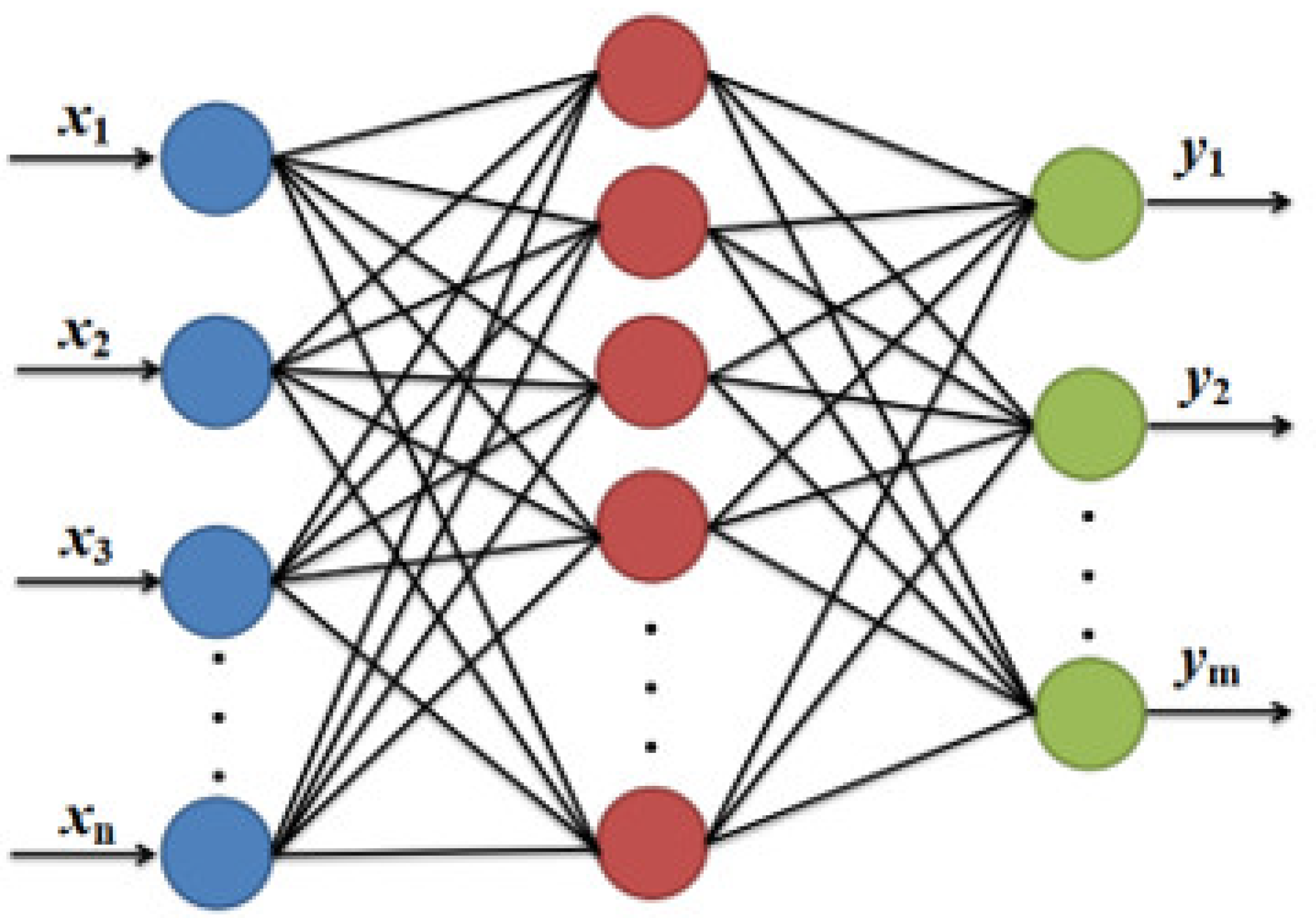
When compared with other feed-forward ANNs, the radial basis function neural network (RBFNN) is effective and provides the best approximation performance and global optimality [
10,
11]. The input, hidden, and output layers are the three layers that make up the RBFNN topology, as shown in
Figure 2 [
12].
To realize nonlinear regression, RBFNN uses the Gaussian function to project the sample from low to high dimension and achieves the linear divisibility of samples [
13].
The output of the hidden layer is calculated as:
where
n is the number of nodes in the input layer;
k is the number of nodes in the hidden layer;
X is the input vector,
n dimension;
xn is the output of the
nth input layer node;
Ci is the center vector of the
ith Gaussian function,
n dimension;
cin is the
ith value of the center vector of the
ith Gaussian function;
||X-Ci|| is the Euclidean distance between the input vector
X and the center vector
Ci of the
ith Gaussian function;
δ is the width of the Gaussian function;
hi is the output of the
ith hidden layer node.
The output of the output layer is calculated as:
where
hi is the output of the
ith hidden layer node;
wij is the connection weight of the
ith hidden layer node and the
jth output layer node;
m is the number of output layer nodes;
k is the number of hidden layer nodes.
If there are
p training samples, then (5) can be written as:
where
Ypj is the output layer output matrix of row
j of
p;
Hpi is the hidden layer output matrix of row
i of
p;
Wij is the output layer weight matrix of row
j of
i.
For convenience, Equation (6) is expanded in the form of a matrix.
where
p is the number of training samples;
j is the number of nodes in the output layer;
i is the number of nodes in the hidden layer;
ypj is the
jth output result corresponding to the
pth training sample;
hpi is the
pth training sample corresponding to the
ith output of the
ith hidden layer node;
wij is the weight of the
jth output layer node corresponding to the
ith hidden layer node.
In Equation (6), the unknown parameter is
Wij. Multiplying the left and right sides of the equation by the inverse or pseudo-inverse of
Hpi,
Wij can be obtained.
When the training samples are used as the centers of Gaussian functions in the hidden layer, the number of training samples is equal to the number of nodes in the hidden layer. At this time, RBFNN is a regularized RBFNN, Hpi in Equation (8) is a square matrix, and the output layer weight matrix Wij is determined by the inverse of Hpi.
4.1.2. Generalized RBNN
When the Gaussian function centers is determined by methods such as k-means clustering, the number of training samples is generally not the same as the number of nodes in the hidden layer, and the RBFNN at this time is a generalized RBFNN. Hpi in Equation (7) is a nonsquare matrix, and the output layer weight matrix Wij can be obtained by the pseudo-inverse of Hpi.
4.2. Radial Basis Function Neural Network (RBFNN)
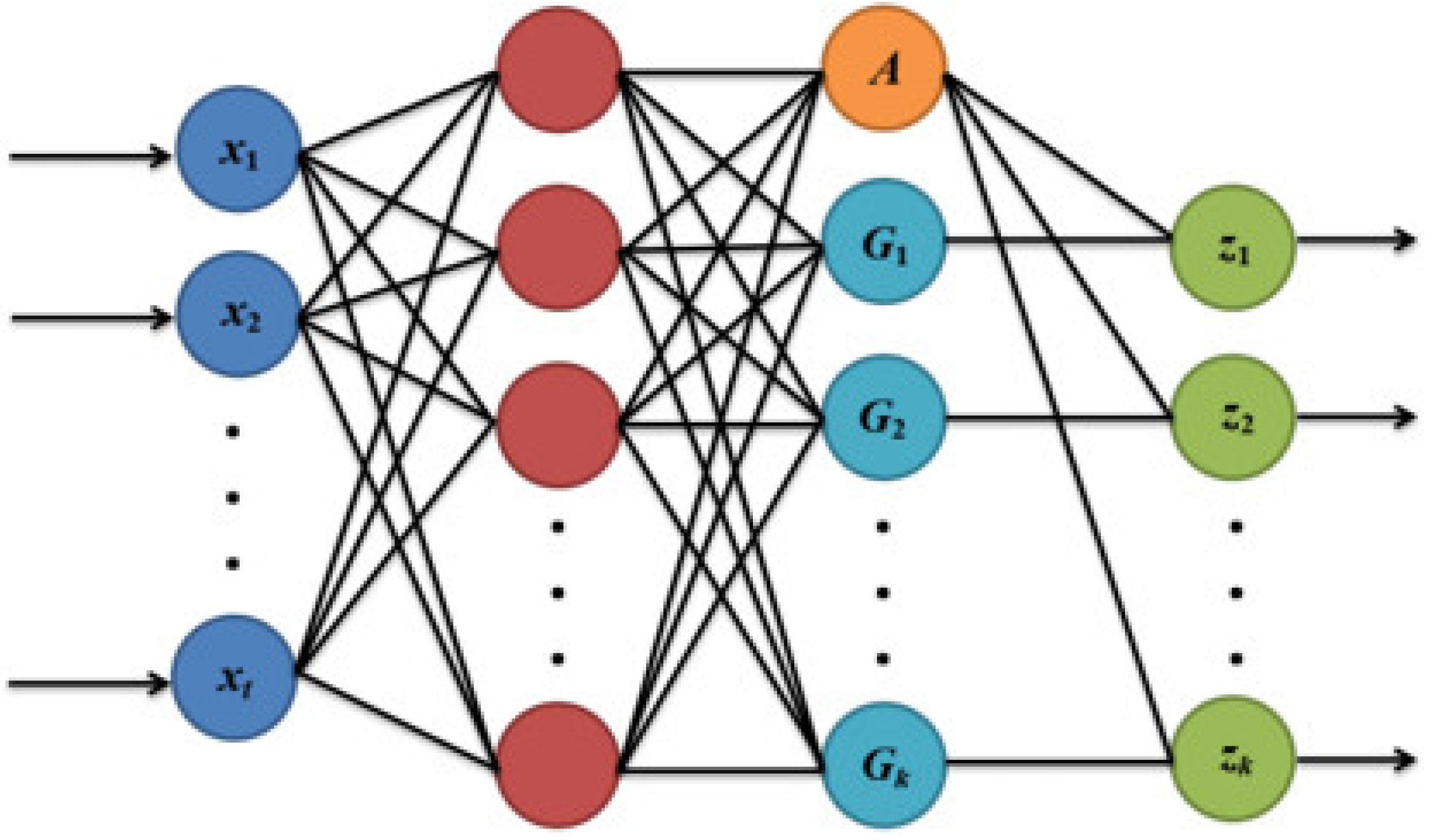
The generalized regression neural network (GRNN), which was developed in 1991 and proposed by Donald Specht [
14], is a neural network model modified from RBFNN [
15]. The GRNN transforms samples using a Gaussian function, projecting the samples from low to high dimensions to achieve linear divisibility, to realize the function from nonlinear nondivisibility to linear divisibility, and then complete the fitting of nonlinear functions and data prediction. The input, hidden, summation, and output layers are the four layers that compose the GRNN structure. In
Figure 3 shows the GRNN topology.
The summation layer is computed differently from the hidden layer, which is similarly computed to the RBFNN hidden layer. The summation layer, which has one more node than the output layer, may be separated into two types of functions, i.e., function
A and function
Gj.
where
A is the output of the summation layer function
A node;
Gj is the
jth output of the summation layer function
Gj node;
q is the number of hidden layer nodes;
k is the number of output layer nodes;
hi is the output of the
ith hidden layer node; and
yij is the
jth value of the real value vector in the
ith training sample.
The output layer nodes are calculated with Equation (11).
where
zj is the output of the
jth output layer node;
Gj is the output of the
jth node of the summation layer function
Gj;
q is the number of hidden layer nodes;
A is the output of the summation layer function
A node;
k is the number of output layer nodes.
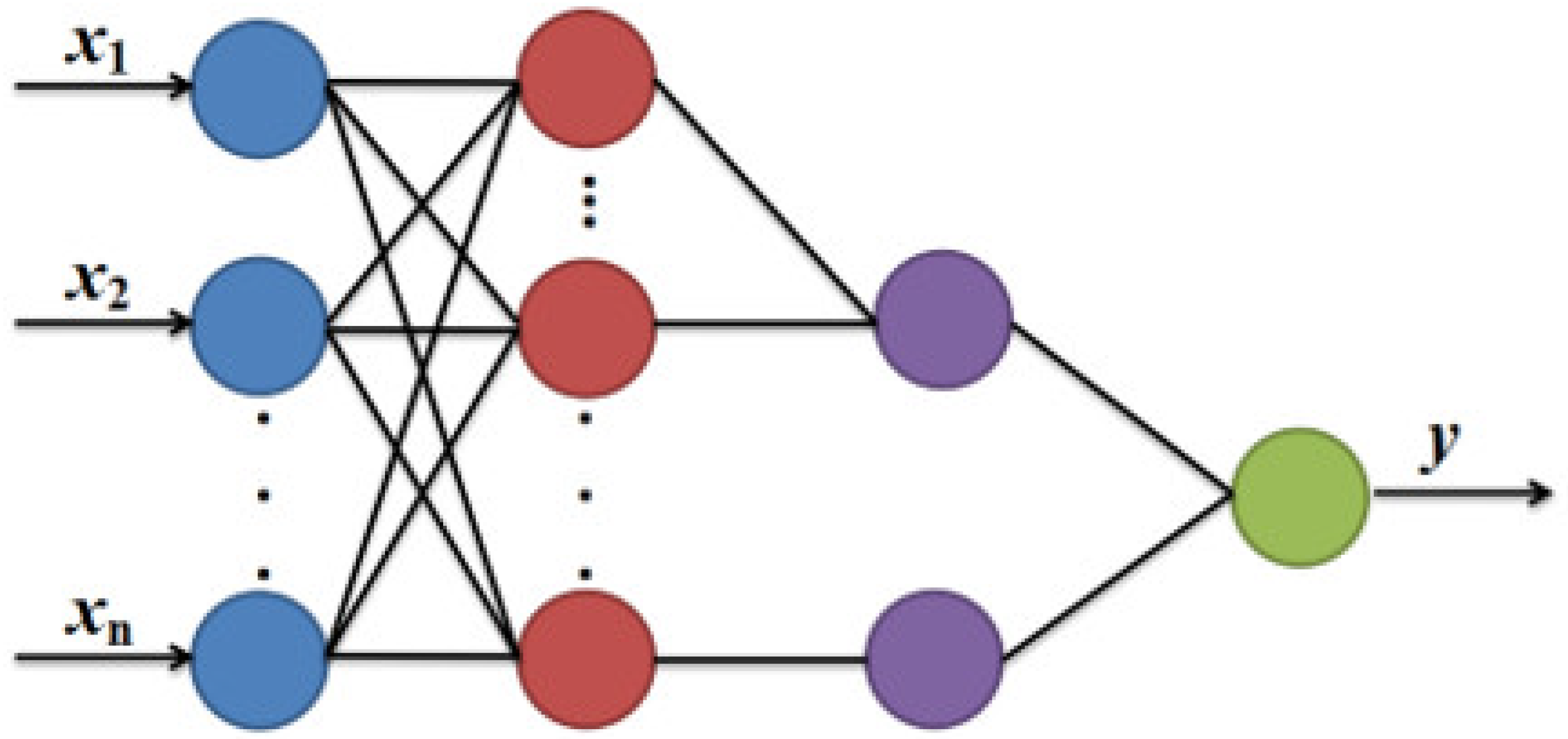
4.3. Probabilistic Regression Neural Network (PNN)
Figure 4 shows the network structure of the PNN, a type of neural network specifically designed for classification.
The same as the RBFNN and GRNN, the hidden layer of PNN is based on the Gaussian function. The competitive layer is used to average the outputs of several hidden layers, compare the size of the competitive layer’s outputs to identify samples with the highest value, and ultimately finish the classification. The value increases with increasing distance from the Gaussian function’s center, while decreasing with increasing distance from it.
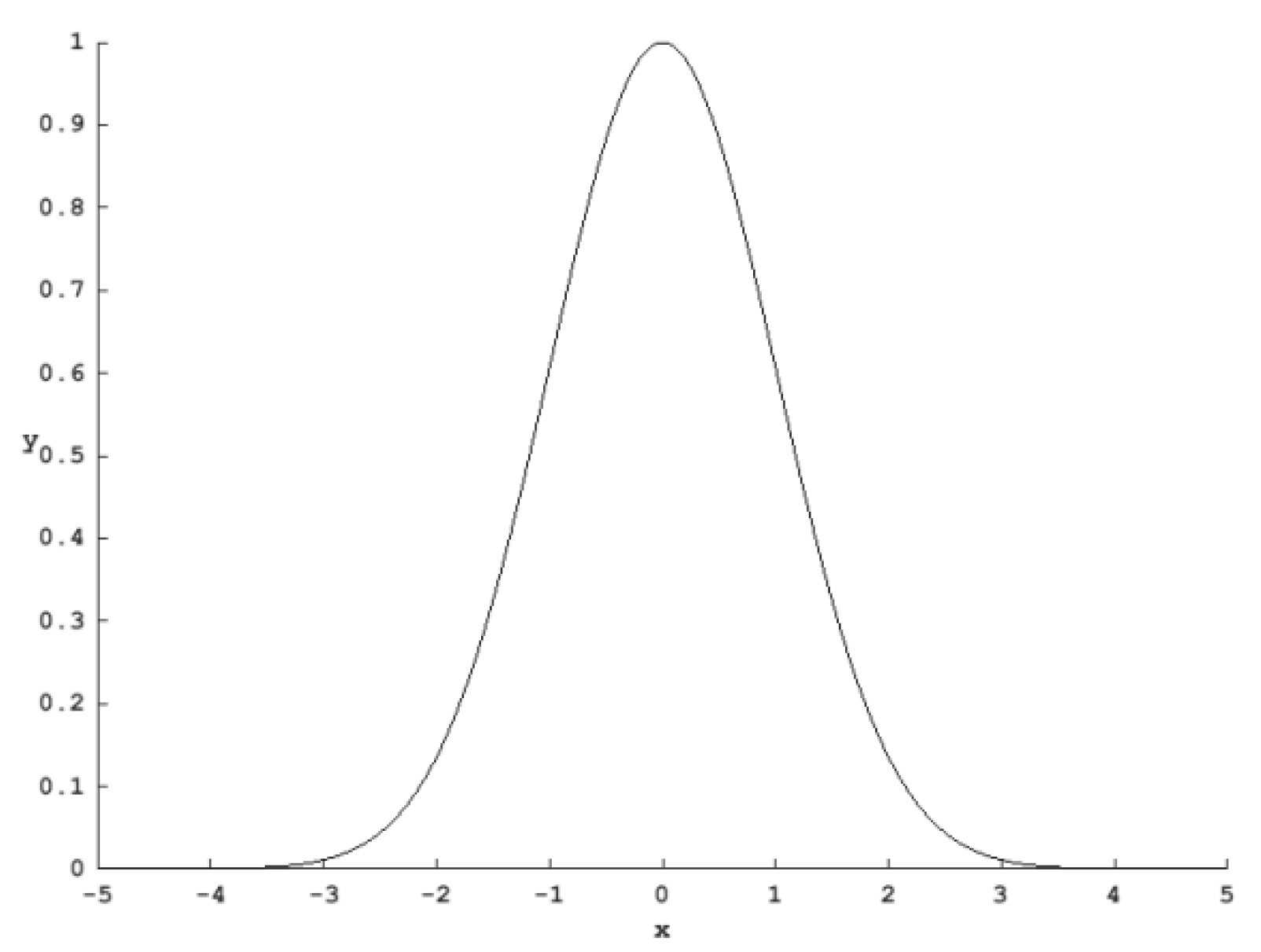
Figure 5 and
Figure 6 show the two-dimensional curves and three-dimensional surfaces of the Gaussian function.
5. Evaluation and Analysis of Prediction Results
5.1. Prediction Results of Normalized RBFNN + k-Means Model
The normalized RBFNN Gaussian function centers and input were created with the 27 groups of clustered samples from the k-means clustering. A brute-force search was used to determine the output layer weights of various Gaussian function centers, resulting in the normalized RBFNN model corresponding to different clustered samples and Gaussian function widths. All the samples in Well-8 were used as the test dataset to evaluate the normalized RBFNN model accuracy and adaptability, so that the best normalized RBFNN model could be determined. As a result, when the Gaussian function center was Clustered Samples 8-1 and the Gaussian function width was 0.52, the prediction accuracy of the test sample was 75.90%, and the prediction accuracy of the kick-state sample was 100%.
In actual operation, kick is unwelcome, i.e., the prediction accuracy of the neural network for kick occurrence must be 100%. At this time, the overall prediction accuracy of the sample was 75.9%, and the other 24.1% inaccuracy was from mistaking the normal state as the kick state, which can simply be replaced by another operation condition and the kick state will not occur. Although the prediction result is conservative, it can guarantee the kick state will not occur to the maximum extent possible, ensuring 100% site safety.
5.2. Prediction Results of Generalized RBFNN + k-Means Model
The generalized RBFNN Gaussian function centers were created with the 27 groups of clustered samples from the k-means clustering. The 226,443 training samples from the seven wells were normalized in accordance with the normalization rule of the 27 clustered samples, and then were employed as the input of RBFNN. A brute-force search was used to determine the output layer weights of the various clustered samples, resulting in the generalized RBFNN model corresponding to several clustered samples. All the samples in Well-8 were used as the test dataset to evaluate the generalized RBFNN model accuracy and adaptability to various clustered samples and Gaussian function widths, so that the best generalized RBFNN model could be determined. As a result, no outcome satisfied the target of the prediction accuracy on the test sample being more than 70%; the prediction accuracy of the kick-state sample was almost 100%.
5.3. Prediction Results of GRNN + k-Means Model
The GRNN Gaussian function centers were created with the 27 groups of clustered samples from k-means clustering. The 226,443 training samples and 40,880 test samples were normalized in accordance with the normalization rule of the 27 clustered samples, and then were employed as the input of GRNN. A brute-force search was used to determine the GRNN model of the various clustered samples. As a result, no outcome satisfied the target of a prediction accuracy on the test sample being more than 70%, and the prediction accuracy of the kick-state sample was almost 100%.
5.4. Prediction Results of PNN + k-Means Model
The PNN Gaussian function centers were created with the 27 groups of clustered samples from k-means clustering. The 226,443 training samples from the seven wells were normalized in accordance with the normalization rule of the 27 clustered samples, and then were employed as the input of PNN. A brute-force search was used to determine the output layer weights of the various clustered samples, resulting in a PNN model corresponding to several clustered samples. All the samples in Well-8 were used as the test dataset to evaluate the PNN model accuracy and adaptability to select the best PNN model. As a result, when the Gaussian function center was Samples 5-2 and the Gaussian function width was 0.41, the normalized PNN had the best prediction result, with 70.16% prediction accuracy on the test sample and 98.75% prediction accuracy on the kick-state sample.
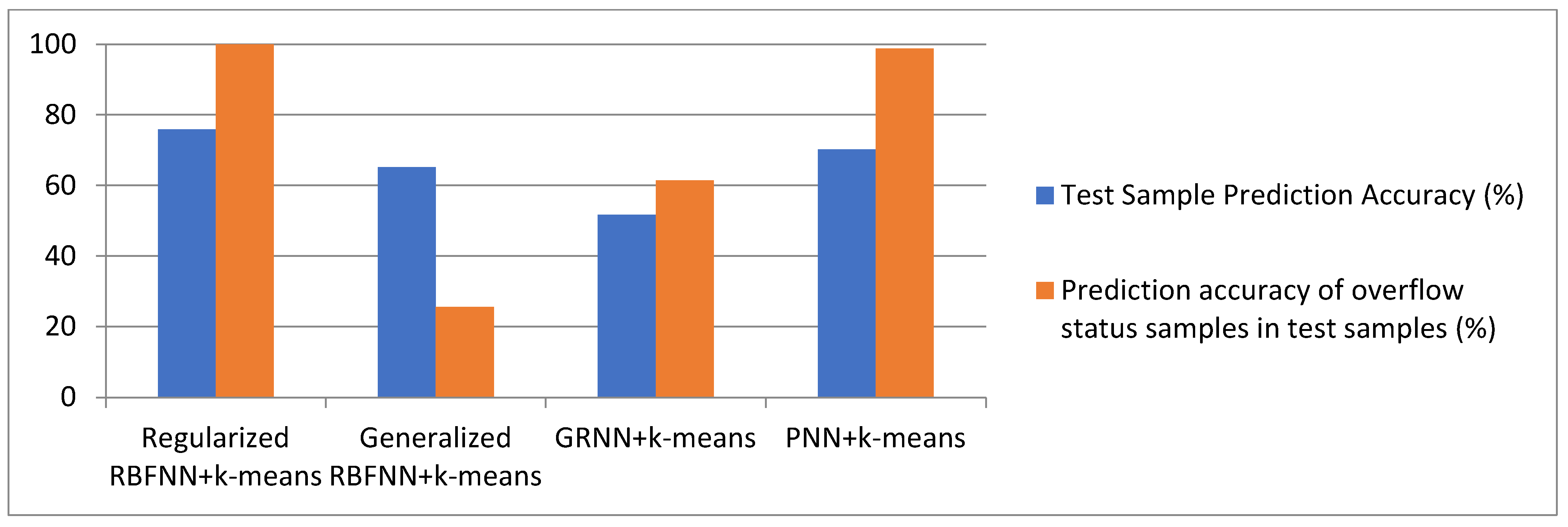
5.5. Comparison of Prediction Results
Table 5 and
Figure 7 show the prediction results of the normalized RBFNN + k-means, generalized RBFNN + k-means, GRNN + k-means, and PNN + k-means models, with the best-clustered samples shown in
Table 2 and
Table 3 above.
The comparison in
Table 5 and
Figure 7 reveals that the regularized RBFNN + k-means model had the best prediction ability, and its prediction accuracy was higher than that of the PNN + k-means model for both the predicted and the kick-state samples in the test samples.
6. Conclusions and Prospect
In this study, field data were clustered with k-means clustering, after which the clustered data were learned and trained for normalized RBFNN, generalized RBFNN, GRNN, and PNN. The prediction results of the four models were then compared and analyzed, and the following conclusions were drawn:
- (1)
Due to the huge volume and similarity of the field data, it was important to cluster the training samples with k-means clustering to decrease data redundancy and accelerate computation speed.
- (2)
After clustering, the data samples were applied in four ANN models, including normalized RBFNN, generalized RBFNN, GRNN, and PNN. According to the comparison and analysis, the normalized RBFNN + k-means model had the highest prediction accuracy.
The limitations of this study are as follows: The neural network’s training samples were derived from k-means clustering calculations. Whether the same number of sample groups was set, the final k-means findings differed, which impacted the neural network’s learning. The neural network should learn these training samples and select the best prediction models with several k-mean computations.
In future work, by introducing kernel principal component analysis (KPCA) or PCA, it will be possible to minimize the dimension of the data while retaining the effects that significantly impact the outcomes and eliminating those that have a minor impact. To more quickly determine the best Gaussian function width, neural network models may also be integrated with intelligent algorithms such as the genetic algorithm (GA), particle swarm algorithm (PSO), and artificial fish swarm algorithm (AFSA).
Author Contributions
Conceptualization, G.Q. and F.X.; methodology, Y.Z.; validation, H.H., F.X. and G.Q.; formal analysis, Y.Z.; investigation, H.H.; resources, H.H.; data curation, Y.Z.; writing—original draft preparation, Y.Z.; writing—review and editing, Y.Z.; supervision, Z.H. All authors have read and agreed to the published version of the manuscript.
Funding
This research received no external funding.
Institutional Review Board Statement
Not applicable.
Informed Consent Statement
Not applicable.
Data Availability Statement
The data presented in this study are available on request from the corresponding author. The data are not publicly available due to their storage in private networks.
Acknowledgments
The authors would like to thank the editor and reviewers for their sincere suggestions on improving the quality of this paper.
Conflicts of Interest
The authors declare no conflict of interest.
References
- Yuan, J.; Fan, B.; Xing, X.; Geng, L.; Yin, Z.; Wang, Y. Research on real-time warning of drilling overflow based on naive bayes algorithm. Oil Drill. Prod. Technol. 2021, 43, 455–460. [Google Scholar]
- Feng, G. Early Monitoring technology of gas well drilling overflow. J. Guangxi Univ. 2016, 41, 291–300. [Google Scholar]
- Codhavn, H.; Hauge, E.; Aamo, O.; Nygaard, G. A novel moel-based scheme for kick and loss mitigation during drilling. J. Process Control. 2013, 23, 463–472. [Google Scholar]
- Guo, Z.; Feng, X.; Tian, D.; Zhang, Y.; Li, Y.; Zhang, C.; Xu, K. EKM overflow warning Intelligent System and its application. Drill. Prod. Technol. 2020, 43, 132–134. [Google Scholar]
- Guo, Y. The data mining method CRISP-DM is used to predict drilling accidents in real time. China Pet. Corp. 2022, 3, 58. [Google Scholar]
- Liu, H.; Li, T.; Zhang, Q. Improved BP Neural network sticking accident prediction based on Adaptive Genetic Algorithm. Mod. Electron. Technol. 2021, 44, 149–153. [Google Scholar]
- Wang, Y.; Haoiasheng, Z.F. Adaptive LSTM warning method for drilling overflow risk. Control Theory Appl. 2022, 39, 441–448. [Google Scholar]
- Fan, X.; Shuai, J.; Li, Z.; Zhou, Y.; Ma, T.; Zhao, P.; Lv, D. Research status and prospect of early overflow monitoring technology in oil and gas Wells. Drill. Prod. Technol. 2020, 43, 23–26. [Google Scholar]
- Zhao, Z.; Deng, H.; Liu, B. Research progress of accident warning in oil drilling engineering. Chem. Eng. Des. Commun. 2021, 47, 180–181+184. [Google Scholar]
- Song, C.F.; Hou, Y.B.; Du, Y. The prediction of grounding grid corrosion rate using optimized RBF network. Appl. Mech. Mater. 2014, 596, 245–250. [Google Scholar] [CrossRef]
- Abulhassan, A. Application of artificial neural networks (ANN) for vapor-liquid-solid equilibrium prediction for CH4-CO2 binary mixture. Greenh. Gases 2019, 9, 67–68. [Google Scholar]
- Zhai, X. Prediction of corrosion rate of 3C steel based on PSO-RBFNN in seawater environment. Corros. Prot. 2014, 35, 1127–1130. [Google Scholar]
- Piun, M.S.; Zhang, Q. Exhaust temperature prediction model of GRNN aero engine based on improved fruit fly algorithm optimization. J. Aeronaut. Dyn. 2019, 34, 8–17. [Google Scholar]
- Duan, C.; Luo, D.; Yang, J. Corrosion rate prediction of refinery pipeline based on KPCA-GRNN. Hebei Ind. Sci. Technol. 2019, 36, 346–351. [Google Scholar]
- Wang, W.; Luo, Z.; Zhang, X. Prediction of Residual Corrosion Life of Buried Pipeline Based on PSO-GRNN Model. Surf. Eng. 2019, 48, 267–275. [Google Scholar]
| Publisher’s Note: MDPI stays neutral with regard to jurisdictional claims in published maps and institutional affiliations. |
© 2022 by the authors. Licensee MDPI, Basel, Switzerland. This article is an open access article distributed under the terms and conditions of the Creative Commons Attribution (CC BY) license (https://creativecommons.org/licenses/by/4.0/).


