Article

Well Construction Action Planning and Automation through Finite-Horizon Sequential Decision-Making

Cockrell School of Engineering, The University of Texas at Austin, Austin, TX 78712, USA
*
Author to whom correspondence should be addressed.
Energies 2022, 15(16), 5776; https://doi.org/10.3390/en15165776
Submission received: 22 June 2022 / Revised: 17 July 2022 / Accepted: 6 August 2022 / Published: 9 August 2022

Abstract

:
Well construction operations require continuous complex decision-making and multi-step action planning. Action selection at every step demands a careful evaluation of the vast action space, while guided by long-term objectives and desired outcomes. Current human-centric decision-making introduces a degree of bias, which can result in reactive rather than proactive decisions. This can lead from minor operational inefficiencies all the way to catastrophic health and safety issues. This paper details the steps in structuring unbiased purpose-built sequential decision-making systems. Setting up such systems entails representing the operation as a Markov decision process (MDP). This requires explicitly defining states and action values, defining goal states, building a digital twin to model the process, and appropriately shaping reward functions to measure feedback. The digital twin, in conjunction with the reward function, is utilized for simulating and quantifying the different action sequences. A finite-horizon sequential decision-making system, with discrete state and action space, was set up to advise on hole cleaning during well construction. The state was quantified by the cuttings bed height and the equivalent circulation density values, and the action set was defined using a combination of controllable drilling parameters (including mud density and rheology, drillstring rotation speed, etc.). A non-sparse normalized reward structure was formulated as a function of the state and action values. Hydraulics, cuttings transport, and rig state detection models were integrated to build the hole cleaning digital twin. This system was then used for performance tracking and scenario simulations (with each scenario defined as a finite-horizon action sequence) on real-world oil wells. The different scenarios were compared by monitoring state–action transitions and the evolution of the reward with actions. This paper presents a novel method for setting up well construction operations as long-term finite-horizon sequential decision-making systems, and defines a way to quantify and compare different scenarios. The proper construction of such systems is a crucial step towards automating intelligent decision-making.

1. Background and Introduction

Well construction, i.e., the process of drilling and completing wells for applications such as extracting hydrocarbons or accessing geothermal energy, is a highly technical discipline. There is irreducible complexity involved in the process while drilling through highly variable geological environments deep in the sub-surface. These environments can pose safety hazards; therefore, the various well construction operations require careful surveillance of the system variables. Currently, real-time (RT) data streams, advanced process models, and sophisticated simulation techniques are utilized for monitoring well construction operations (see e.g., [1]). Decision-making, however, is still primarily performed by humans, with little automation. The decisions are based on the understanding of the processes by the subject matter expert (e.g., engineer, or the driller out in the field) in control of the process. They are made not only based on interpretations of the model outputs, but also to a large extent on past experiences, and sometimes ‘gut feelings.’ The decisions are also affected by other human factors, such as situational awareness or even the physical and mental state of the decision-maker (with, e.g., fatigue playing a major role [2]). The consequences of making erroneous decisions can range from poor operational efficiency to catastrophic failures and accidents.
The overarching goal of the research presented here is the development of an automated intelligent decision-making system for improved well construction safety and performance. Developing such a system requires the identification of the necessary data and data streams, digital twinning of the underlying operation, structuring the decision-making system, and finally selecting the simulation or planning method. This paper discusses a general approach for setting up such systems by combining data and digital twins, and demonstrates this for hole cleaning operations. Hole cleaning is the process of removing solids (cuttings generated during drilling, cavings, or metal shavings) from the borehole to ensure that different well construction operations (including drilling, tripping, casing installation, and cementing) can be performed safely and efficiently. Inefficient hole cleaning can result in various problems, such as stuck pipe, downhole tool damage, formation damage, or trouble running the casing. Hole cleaning issues account for several hundred million dollars annually in lost time costs [3,4]. The literature on hole cleaning modelling is extensive; the latest developments are covered in detail by [5] and references therein. There is, however, currently no framework for setting up systems that can perform scenario analysis and action planning in well construction processes such as hole cleaning, and this is the main topic of this paper.
In other domains, the use of sophisticated decision-making systems has resulted in an overall improvement in safety and operational efficiency. Such decision-making systems, coupled with digital twins of operations or equipment, have been utilized in areas such as manufacturing [6], autonomous vehicles [7,8], and smart grid management [9,10]. Recently, high-complexity board games (e.g., go and chess) were solved using tree-based search techniques in combination with learned system models [11,12]. Complex RT strategy games, such as StarCraft and Dota, have been solved by utilizing novel reinforcement learning techniques [13,14]. Amongst these, sequential decision making is a class of algorithm that takes the dynamics of the system into consideration. The decision and actions are made in steps, and adjusted based on rewards assigned to outcomes. This approach parallels how manual decisions and actions are made with regards to hole cleaning in an actual drilling operation, which motivated its selection as the approach of choice in this paper. Further, given the need to arrive at a solution within a certain time period, the hole cleaning problem is handled as a finite-horizon sequential decision-making problem.

2. Setting up the Planning and Decision-Making Systems for Well Construction Operations

Planning is the process of generating an action sequence from an initial system state to some goal state to satisfy some high-level objective function. Multiple approaches such as forward search algorithms (A* search, greedy best-first search, Dijkstra’s algorithm), exhaustive methods (tree search, policy iteration, value iteration), or simulation-based search methods (flat Monte Carlo, Monte Carlo tree search) can be used to solve planning problems [15,16,17]. Most of these methods utilize a combination of domain knowledge and logic with search functions, which can be further enhanced by heuristics. This paper does not cover the algorithm selection process, and the reader is referred to [18] for a detailed comparison of the approaches. The various planning algorithms were evaluated using six criteria, namely optimal solution guarantee, memory requirement, computational time requirement, necessity of a well-defined admissible function, evaluation function use, and exploration/exploitation balancing. All planning problems, however, have the following essential components [15]:
-
Objective function, stating the initial and the desired (goal) states, and constraints that can influence decision-making;
-
Decision epochs, or the times at which decisions need to be made. Epochs can either be explicitly represented as time intervals, or implicitly represent a sequence of actions in succession;
-
State space, to describe all possible situations or scenarios (states) the system can be in, at any given decision epoch;
-
Action space, to quantify all possible decisions or actions that can be utilized to manipulate states;
-
Plan, or strategy that represents the sequence of actions taken at every successive decision epoch.
In effect, planning problems are sequential decision-making problems that can be solved by reinforcement learning (RL) techniques. In RL, a goal-directed learning agent interacts with an uncertain environment (either physically or virtually) based on specific policies or action plans. Every interaction is associated with immediate feedback or reward. The goal of this agent is to maximize the long-term reward. To accomplish this, the agent needs to exploit what it has already experienced and try new actions to learn from unexplored trajectories [19,20]. Figure 1 shows a schematic of this agent–environment interaction, where an action a t by the agent in the environment (observed by the agent to be in state s t ) results in an immediate reward r t and a new observed state s t + 1 .
Such interactions between a decision-making agent and a fully observable environment to achieve some long-term objective can be formalized in a Markov decision process (MDP) framework. A process is said to be Markovian if it follows the Markovian property, i.e., if any future outcomes depend only on the current system state and the immediate action. An MDP is defined by a tuple ( { S , A , P , R } ) and a policy ( π ) [21].
S is the state space, where s t ( s t S ) represents the state of the system, as perceived by the agent, at time t . A state is defined by a set of parameters to quantify the condition of the environment completely (fully observable). A is the action space, where a t ( a t A ) is an individual action taken by the agent at time t to manipulate the system in the state s t . An action is a combination of different control variables that can influence the environment. P is the transition function representing the state–action transition probabilities. P s s a is the probability that a system in state s , at time t transitions to state s at time t + 1 on taking an action a . R is the reward function to quantify the immediate feedback associated with a state–action transition. Reward may depend either only on the final state, or on the final state and the action.
The accumulation of rewards over multiple time steps or decision epochs is the system’s return. The time horizon for accumulating these rewards may be finite (fixed number of steps) or infinite, and may include a discount factor γ (≤1) in the case of infinite time horizon problems. In this paper, we assume 10 finite steps and therefore assume a discount factor ( γ = 1 ), giving every step equal weight. The policy π is the logic or set of rules used by an agent to select an action from a given state; it may be stochastic or deterministic. The goal of an agent is to find a policy that allows it to maximize its total return. There is always at least one optimal policy for an MDP that helps extract the maximum return from the system [22]. Another crucial step in MDP formulation is reward shaping, or engineering the reward function to obtain more frequent feedback on appropriate system behaviors [23]. Thus, reward shaping influences the total return, thereby affecting the system’s policy.

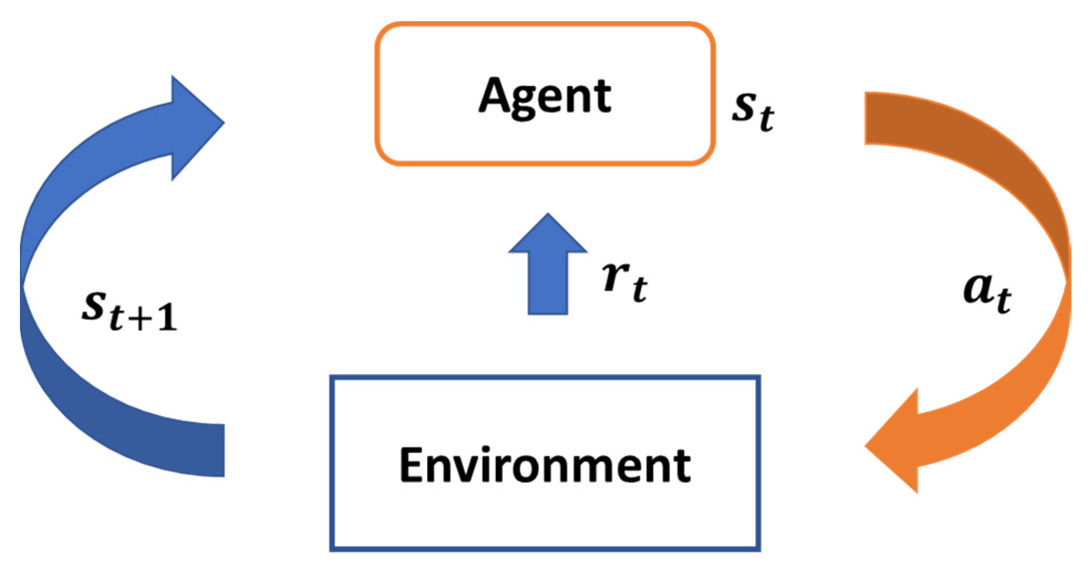
2.1. Well Construction Sub-Processes as MDPs

Well construction is a multi-step process that requires planning and decision-making at every step of its various sub-processes. Planning necessitates identifying objectives, constraints, and required data associated with the individual sub-processes. A crucial step in developing such planning systems is setting them up properly, which requires the following elements:
-
Formulating an MDP for the operation, which includes appropriately defining state and action spaces
-
Defining a goal or a desired state
-
Efficient shaping of the reward function
-
Setting up an integrated-multi model system replicating the process (environment), i.e., building its digital twin

2.1.1. MDP Formulation

Formulating an MDP for any process requires the following [21]:
-
The process should satisfy the Markovian property
-
Any state defined for the process should be fully observable
-
State space should be finite or countably infinite, with states defined by exhaustively incorporating all relevant parameters
-
There is an explicit definition of the action space with appropriately identified control variables
For most well construction processes, the condition (state) of the wellbore at any time is a culmination of all the previous operations (actions), past conditions (past states), and state transitions. In other words, the current state is a representation of the well’s operational past, and any subsequent transition depends only on this state and the immediate action. The assumption that well construction operations follow the Markovian property is, therefore, valid. The state of the system needs to be represented by all relevant parameters required to fully describe the process under consideration. The state is also continually refined based on the data received from surface or downhole sensors (at frequencies of 1 Hz or higher). This results in the state being a complete representation of the environment as perceived by the agent, i.e., the state is assumed to be fully observable. The operations or variables that can be actively controlled to bring about state transitions constitute the action.
The state and action spaces can be either discrete or continuous; however, for the work presented here, both are defined as discrete sets. Figure 2 illustrates the proposed method for discretizing the state space based on wellbore inclinations. Well inclinations in the range 0 to 30 degrees are considered to be a near-vertical section, and the regions of the well with inclination angles greater than 75 degrees are considered to be near-horizontal lateral. The intermediate inclination angle regions comprise the curve or the build section of a well. This method of discretizing the state space is proposed because the response of state variables to different actions has a high degree of dependency on the inclination of the well segment. Wellbore inclination significantly influences the cuttings transport mechanisms, which are different for near-vertical, intermediate, and lateral sections. Consequently, this affects the hole cleaning requirements. Note, however, that the state space may be discretized in other ways, such as in intervals or sections of measured depth (MD) or true vertical depth (TVD).
Equation (1) represents the state vector, where ‘ p 1 ’ through ‘ p n ’ are the exhaustive set of parameters required to define the system state completely. The state of the system here consists of some functional value of these parameters over the appropriate inclination intervals { [ 0 , 30 ) , [ 30 , 45 ) , [ 45 , 60 ) , [ 60 , 75 ) , [ 75 + ) } . Another point to note is that these inclination interval definitions can be adjusted depending on the requirements of the underlying process.
s t = { p 1 _ 0 30 p 1 _ 30 45 p 1 _ 45 60 p 1 _ 60 75 p 1 _ 75 + . p n _ 0 30 . p n _ 75 + }
Similarly, the action space is constructed by different combinations of possible values of the identified control variables. For drilling operations, some such control variables are the surface drillstring rotation speed (RPM), weight on bit (WOB), drilling mud properties, flowrate, and drillstring tripping speeds. These variables can take on discrete values between specified minimum and maximum thresholds. These thresholds are dictated by safety constraints, process and equipment limitations, and operational economics. Note that in some problems, it will make more sense to break down the problem by measured depth or true vertical depth sections instead of by inclination. Additionally, the state space parameters will be dependent on the objective of the digital twin. In this paper, the parameters were largely dictated by the hole cleaning/hydraulics problem, serving as an example of how the problem can be mathematically set up for action planning.

2.1.2. Goal State

The goal or desired state, as the name suggests, refers to the subset of the state space that the drilling agent aims to achieve. The goal state is used as the reference to direct the agent’s search. The desired functional values of individual goal state components are used for the construction of the overall goal state, as shown in (2).
s g o a l = { p g 1 _ 0 30 p g 1 _ 30 45 p g 1 _ 45 60 p g 1 _ 60 75 p g 1 _ 75 + . p g n _ 0 30 . p g n _ 75 + }

2.1.3. Reward Shaping

Shaping the reward function allows for rewarding or penalizing a drilling agent’s behavior more frequently, instead of at sparse intervals or at the end of an episode. Frequent rewards, in turn, help with more directed and faster learning. A possible strategy for reward shaping is to provide the agent with regular feedback based on its position relative to the goal state. Another factor to consider is the contribution to the reward of the relative changes in different action control variables. For instance, if a state transition from s to s can be achieved by two completely different actions a and a , the reward function needs to be able to recognize and quantify this difference. This is especially important, for instance, in cases where the agent suggests changing drilling RPM and flowrate with an alternative action being a change to mud rheological parameters (which may be economically and temporally more expensive).

2.1.4. Digital Twinning the Environment

For action planning, a comprehensive model or digital twin of the process needs to be constructed. This twin is then used for replicating the environment, thereby simulating multiple episodes or trajectories of experience [6,24,25]. Model-free RL techniques can then be applied to these episodes to improve the return value and, subsequently, to determine an optimal policy. Figure 3 details these steps. The Monte Carlo tree search approach was identified to be applicable to this problem and is discussed in detail in [25].

3. Setting up the Hole Cleaning Decision-Making System

Here, we demonstrate step-by-step how to set up a decision-making and planning system for the hole cleaning operation.

3.1. Formulating the MDP for the Hole Cleaning System
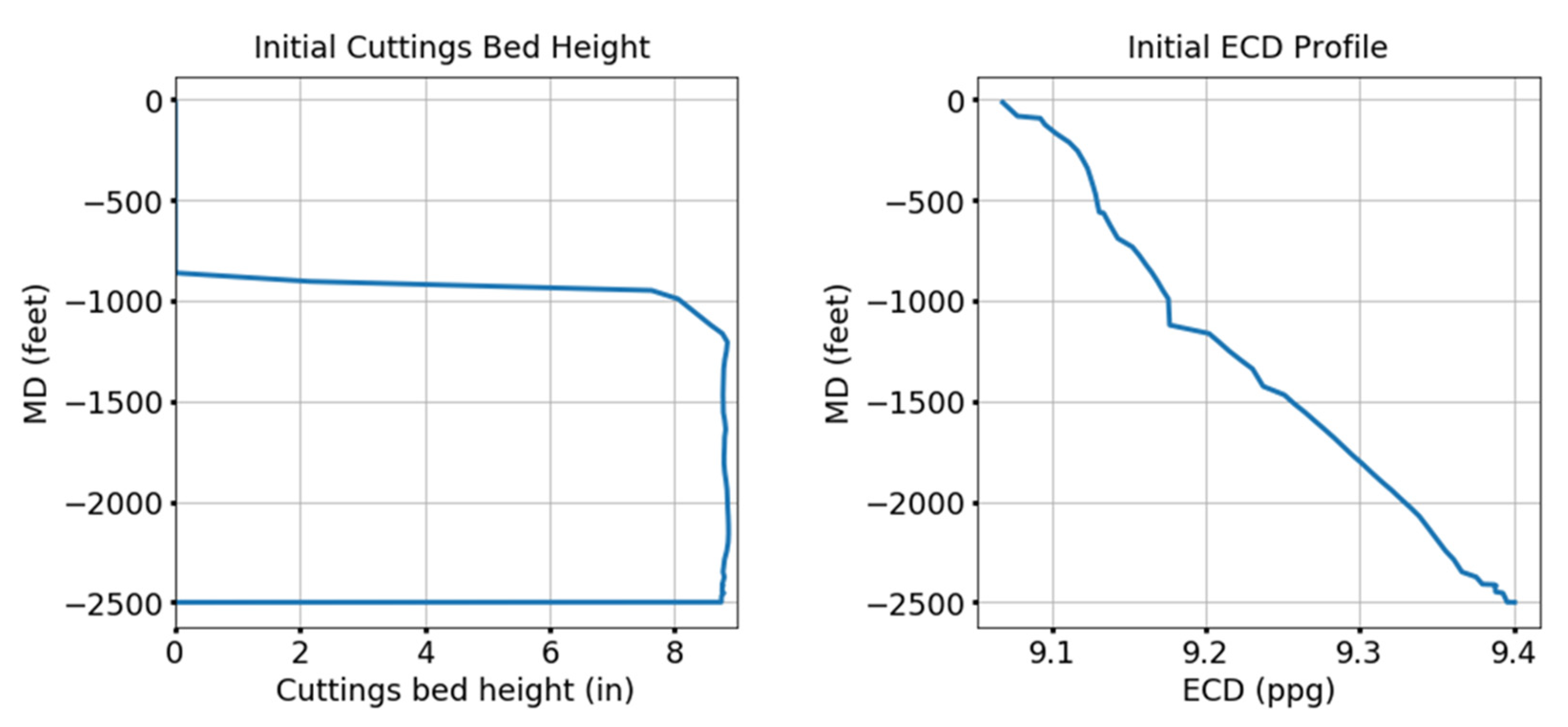
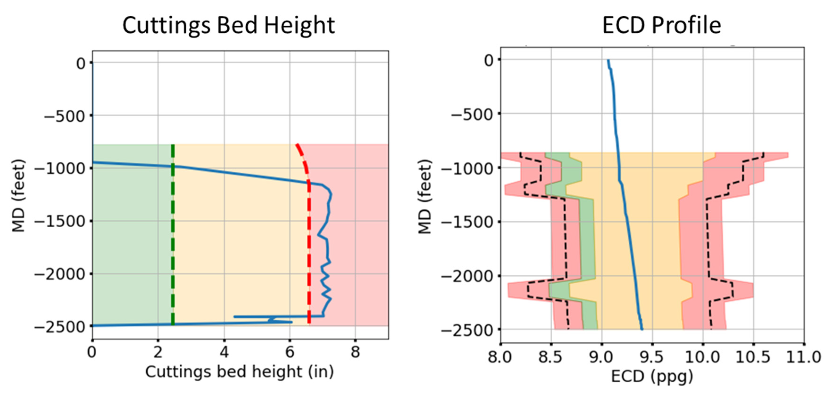
Effective and safe hole cleaning requires keeping the cuttings bed height low enough to prevent issues at any stage of the well construction operation. Moreover, the equivalent circulation density (ECD) needs to be managed within a safety or drilling margin (Figure 4). ECD at a depth is the gradient of the sum of the hydrostatic head exerted by the drilling mud (a function of the true vertical depth (TVD) of the well) and the total circulating frictional pressure loss in the annulus between the drillstring and the wellbore, which is a function of the measured depth (MD) along the length of the well [26].
ECD = P hydrostatic _ D TVD + P frictional _ pressure _ loss _ D MD D TVD · g
In Figure 4a, the lower and upper limits of the drilling margin are the stability limit (SL) and the fracture gradient (FG), respectively. SL is the higher value between the pore pressure (PP) and the mud pressure essential for maintaining wellbore stability. PP is exerted by the fluids (brine or hydrocarbons) present in the pore spaces of the formation rocks. If the ECD falls below the SL, it can cause wellbore instability and, if it falls below the PP of permeable formations with the potential to flow, an unwanted influx of formation fluids into the borehole (which is called a ‘kick’). Exceeding the FG can fracture the formation and lead to mud loss. Such mud loss events are called lost circulation events [27]. It is, therefore, an objective of the system to maintain the ECD within this drilling margin at all times.
Figure 4b depicts the cuttings bed distribution in the different sections of the wellbore. In the near-vertical section of the wellbore, the principal method of suspending and carrying cuttings up hole in the mud is by overcoming the particle slip velocity, and no cuttings bed can exist. In the curve section (inclinations from 30 to 60 degrees), an unstable cuttings bed can form below the angle of repose. However, there is a high possibility that when the mud circulation stops, the cuttings avalanche back down the annulus, which can pack off around the bottom-hole assembly, causing a stuck pipe incident. For this section, the hole cleaning design requires tackling and preventing this cuttings avalanche. In the near-horizontal section (inclination angle from 60 to 90 degrees), above the angle of repose for the cuttings, a stable cuttings bed will form on the low side of the hole. The primary hole cleaning requirement is to continuously move this bed up and out of the hole (see e.g., [28,29]). Therefore, another main objective of the decision-making system is to satisfy these hole cleaning requirements.

3.1.1. State Space

The following parameters are required to quantify the condition of the borehole from the perspective of the hole [30,31]:
-
Height of the cuttings bed in the curve and the lateral sections of the wellbore;
-
ECD along the entire length of the wellbore.
The well can be treated as a series of interconnected control volumes, segmented based on any changes in well dimensions (e.g., changes in inner or outer diameters) or based on different survey intervals (as shown in Figure 4b). Each control volume’s condition can be independently represented by absolute values of ECD and cuttings bed height. However, with the well being segmented into multiple inclination intervals (based on the strategy discussed in Figure 2), every inclination interval usually consists of many such control volumes. A functional value derived from the absolute value is calculated for each of these parameters in every control volume. These values are then averaged over the different inclination segments to obtain a single value per inclination interval for every parameter. Converting to a functional value normalizes the absolute value to specific operational thresholds, and assists in reward shaping, as discussed in later sections.

Cuttings Bed Height

The absolute value of the cuttings bed height for every control volume is normalized to its outer diameter (Figure 5). These values are then used to calculate the average normalized cuttings bed height indicator H (dimensionless) for every inclination segment of the well, as shown by Equation (4).
H k n o r m = H k a b s o l u t e D o _ k ,   H = k = 1 N s e g H k n o r m N s e g
The functional value H i n c . is then derived from H using Equation (5), as visualized in Figure 6.
H i n c . = { 0 H 0.20 1 0.20 < H 0.40 2 0.40 < H 0.60 3 0.60 < H 0.80 4 H > 0.80
The parameter H i n c . is evaluated for all non-vertical sections, because no cuttings bed will form in the [ 0 , 30 ) degree inclination interval. Thus, the bed height components of the state vector are { H 30 45 , H 45 60 , H 60 75 , H 75 + }.

ECD

As previously discussed, ECD needs to be managed within the drilling margin. There is, however, some degree of uncertainty associated with its limits, which is accounted for by considering an uncertainty factor D F ( 0.25 ) . ECD a v g , the average ECD for an inclination interval, is calculated by averaging absolute ECD values over all the control volume segments in that interval (Equation (6)). Since the SL and FG values vary with depth, ECD a v g is calculated independently for the different intervals.
ECD a v g = k = 1 N s e g ECD k a b s o l u t e N s e g
Using ECD a v g , the functional value of ECD, ECD i n c . , is calculated using Equation (7) and discussed in Figure 7.
ECD i n c . = { 3 ECD a v S L D F · Δ w 2 S L D F · Δ w < ECD a v S L 1 S L < ECD a v S L + D F · Δ w 0 S L + D F · Δ w < ECD a v S L + 2 · D F · Δ w 1 S L + 2 ·   D F · Δ w < ECD a v F G 2 · D F · Δ w 2 F G 2 · D F · Δ w < ECD a v F G 3 ECD a v > F G w h e r e Δ w = F G S L
Since keeping ECD within the drilling margin is essential throughout the well, the state components related to the ECD parameter, { ECD 0 30 , ECD 30 45 , ECD 45 60 , ECD 60 75 , ECD 75 + } are calculated for all intervals.
Equation (8) represents the complete hole cleaning state of the wellbore. In this form, every component of the state vector is represented by its functional value at every decision epoch.
s = { H 30 45 H 45 60 H 60 75 H 75 + ECD 0 30 ECD 30 45 ECD 45 60 ECD 60 75 ECD 75 + }
This representation of state is Markovian since it fully represents the condition of the hole cleaning system and encompasses all the information about the system’s history. Any subsequent state transition depends only on the state and the action taken. As can be seen from Equation (8), the state vector has nine parameters. Each of the H i n c . parameter can have five values while each of the ECD i n c . parameters can have seven values. This translates into a state space size of 54 × 75 = 10,504,375.

3.1.2. Goal State

The goal for any decision-making system is to first search the state and action space and then move towards the desired state. The functional values for all state variable components are defined such that 0 represents the desired state for each; therefore, the target goal state for the system is as shown in Equation (9).
s g o a l = { 0 0 0 0 0 0 0 0 0 }

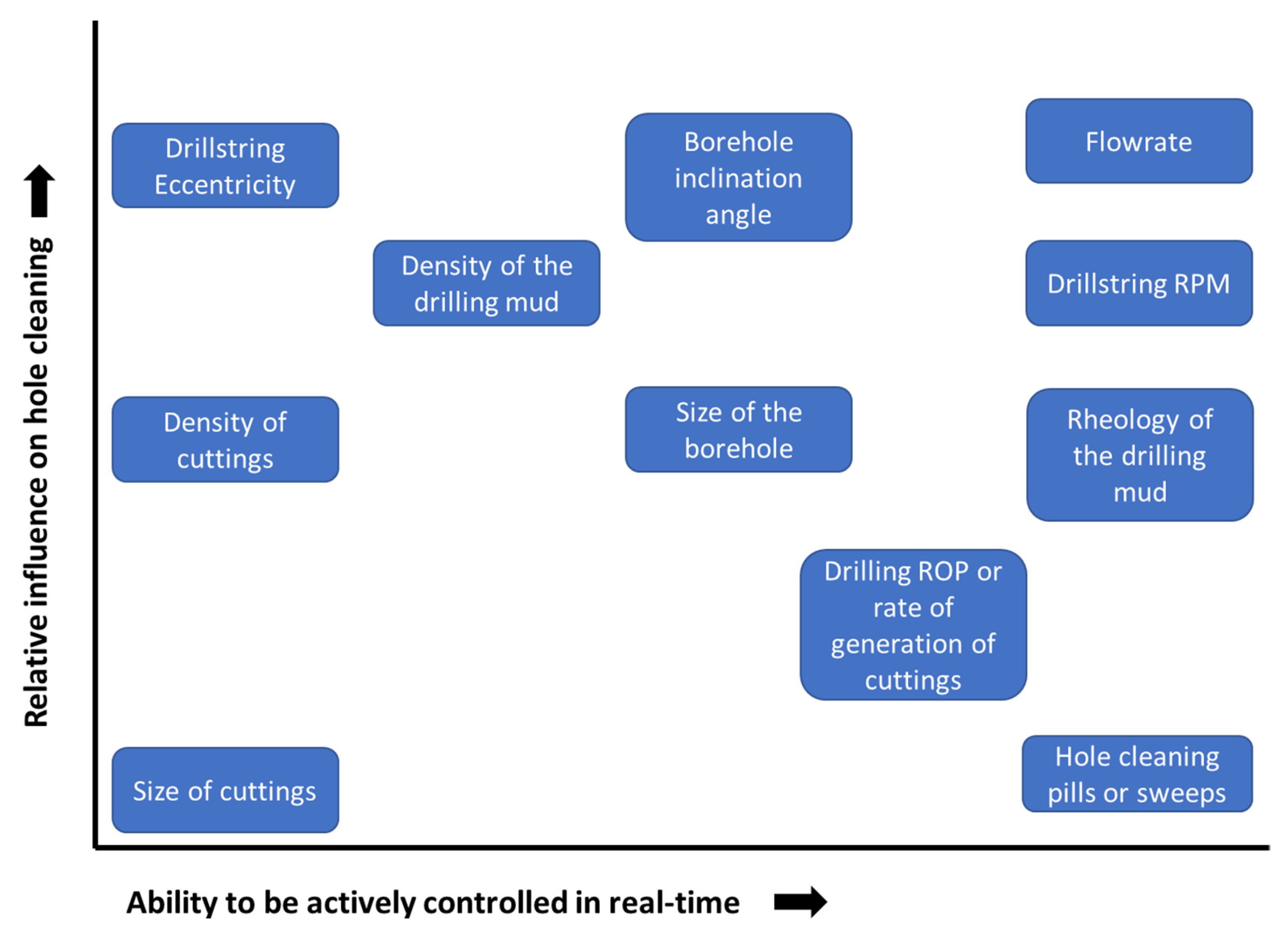
3.1.3. Actions Space

Hole cleaning, while managing the ECD within the drilling margin, is a function of (see e.g., [32,33,34]:
-
Drilling mud properties (particularly density and viscosity);
-
Cuttings properties (size and density);
-
Drilling parameters such as drilling RPM and flow rate;
-
Drillstring geometry and its eccentricity in the borehole;
-
Rate of cuttings generation (which depends on the drilling rate);
-
Borehole geometry (diameters of the open or cased hole sections along the well) and inclination angle.
Hole cleaning pills or sweeps, i.e., limited volumes of fluid with altered density and/or viscosity to aid in cuttings evacuation from the hole (mostly effective in vertical hole rather than deviated hole).
Some of these control variables affect the condition of the borehole to a greater extent than others. Moreover, some variables can be controlled more readily than others. Figure 8 presents a chart comparing the different control variables, plotted for their relative influence on hole cleaning against their ability to be actively controlled in real-time.
Thus, the key parameters that have a significant influence on the hole cleaning performance, and can be actively controlled in the field, are flow rate, RPM, mud properties (rheological parameters), and the WOB to control the rate of penetration (ROP). In the following, we will assume that the fluid behavior is that of a Bingham plastic fluid, in which case its rheology is quantified by its plastic viscosity (PV) and yield point (YP). Another critical parameter that influences the ECD is the mud density. A combination of these variables at every decision epoch constitutes an action, which is represented by Equation (10).
a t = { F l o w r a t e R O P R P M M u d   d e n s i t y M u d   P V M u d   Y P }

3.2. Digital Twin of the Environment

A digital twin was built by integrating the available well initializations (data streams such as well plans, well surveys, well geometry information, etc.) with analytical implementations of the hydraulics and cuttings transport models [18]. The hydraulics model calculates the frictional pressure losses and ECD throughout the well and utilizes sub-models presented in [32,36]. The cuttings transport model also utilizes multiple sub-models [37,38,39,40,41,42,43] and estimates the cuttings bed height and the cuttings concentration in the flow stream along the well. Figure 9 illustrates the use of this twin to predict the system state at the next epoch, based on the current state and immediate action. The epoch is the smallest time step of the planning problem for which an action is determined. The digital twin was designed to plan either every 5 min interval into the future or whenever there was a change in the well operations.

3.3. Reward Function

To quantify the immediate feedback associated with state–action transitions, a reward function is defined for the hole cleaning system, which has three distinct components:
-
Reward associated with state transition;
-
Penalty associated with action transition;
-
Reward associated with action variables.

3.3.1. Reward Associated with State Transition

Since the objective of the system is to reach the goal state, every component of the state vector tries to achieve a functional value of 0. This was used as a reference to calculate normalized reward values associated with every state vector component in the [ 1 , 1 ] range. Table 1 details the functions used for these calculations.
Thus, the reward function contribution of state transition is represented by the set given in Equation (11).
R S = { R H 30 45 , R H 45 60 , R H 60 75 , R H 75 + , R ECD 0 30 , R ECD 30 45 , R ECD 45 60 , R ECD 60 75 , R ECD 75 + }

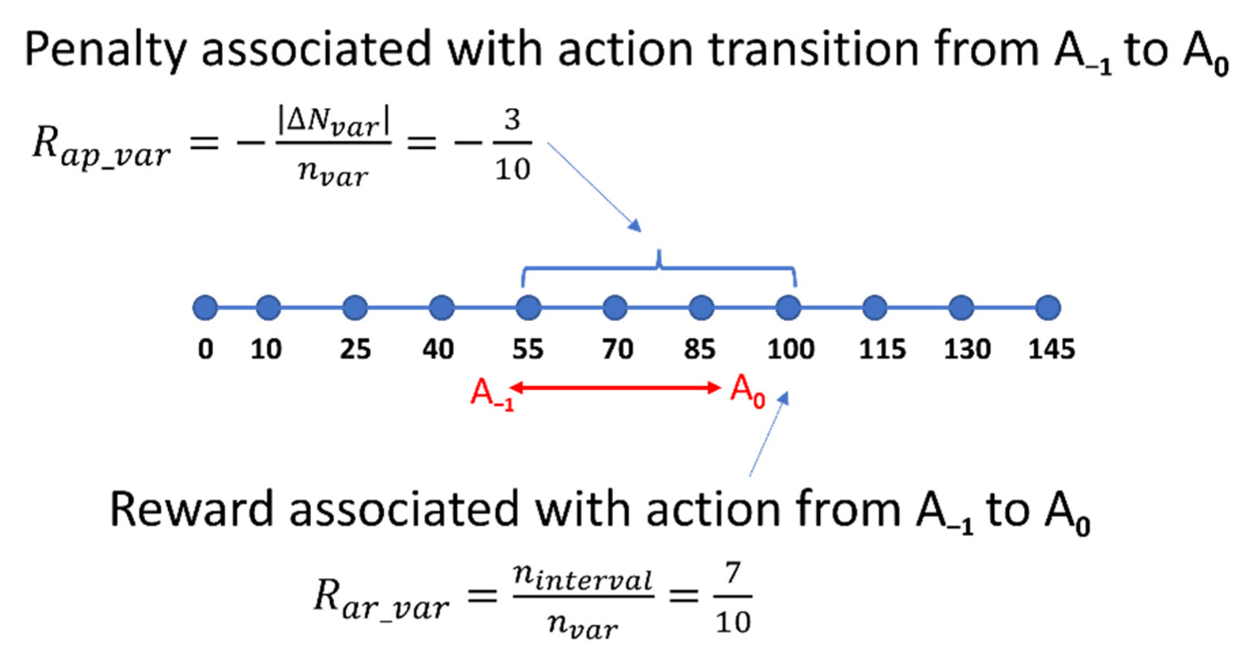
3.3.2. Penalty Associated with Action Transition

Table 2 details the calculation of the penalty (negative reward) related to changes in action values. The purpose of these definitions is two-fold:
-
To discourage the system from making extreme changes in actions, unless the reward associated with state transition offsets this penalty;
-
Select the least penalizing action in case multiple actions result in the same state transition.
The terms Δ N v a r i a b l e and n v a r i a b l e , respectively, are the number of interval changes between consecutive actions and the number of discrete values possible for a given control variable. Their use to calculate a penalty value is illustrated in Figure 10. Here, the action results in a jump across 3 out of a total of 10 intervals and therefore the penalty is −3/10. The action transition-based penalty set is expressed in Equation (12).
R a p = { R f l o w r a t e , R R O P , R R P M , R d e n s i t y , R P V , R Y P }

3.3.3. Reward Associated with Action

In the planning phase of drilling operations, the hole cleaning requirement of the system would push the ROP to zero, simply because no cuttings are generated at zero ROP leading to zero bed height and optimum ECD. However, because a critical objective of drilling is to drill a well as fast as reasonably possible (within given limits), there needs to be a positive feedback or reward associated with the ROP. Equation (13) represents this reward, which is calculated using Equation (14) as a ratio of the discrete interval number for a given ROP value to the total number of ROP intervals. This reward component is in the range [ 0 , 1 ] . The calculation is also illustrated in Figure 10. The action results in a jump to the seventh interval and therefore the reward is 7/10.
R a r = { 0 , R R O P , 0 , 0 , 0 , 0 }
R R O P = n i n t e r v a l n R O P

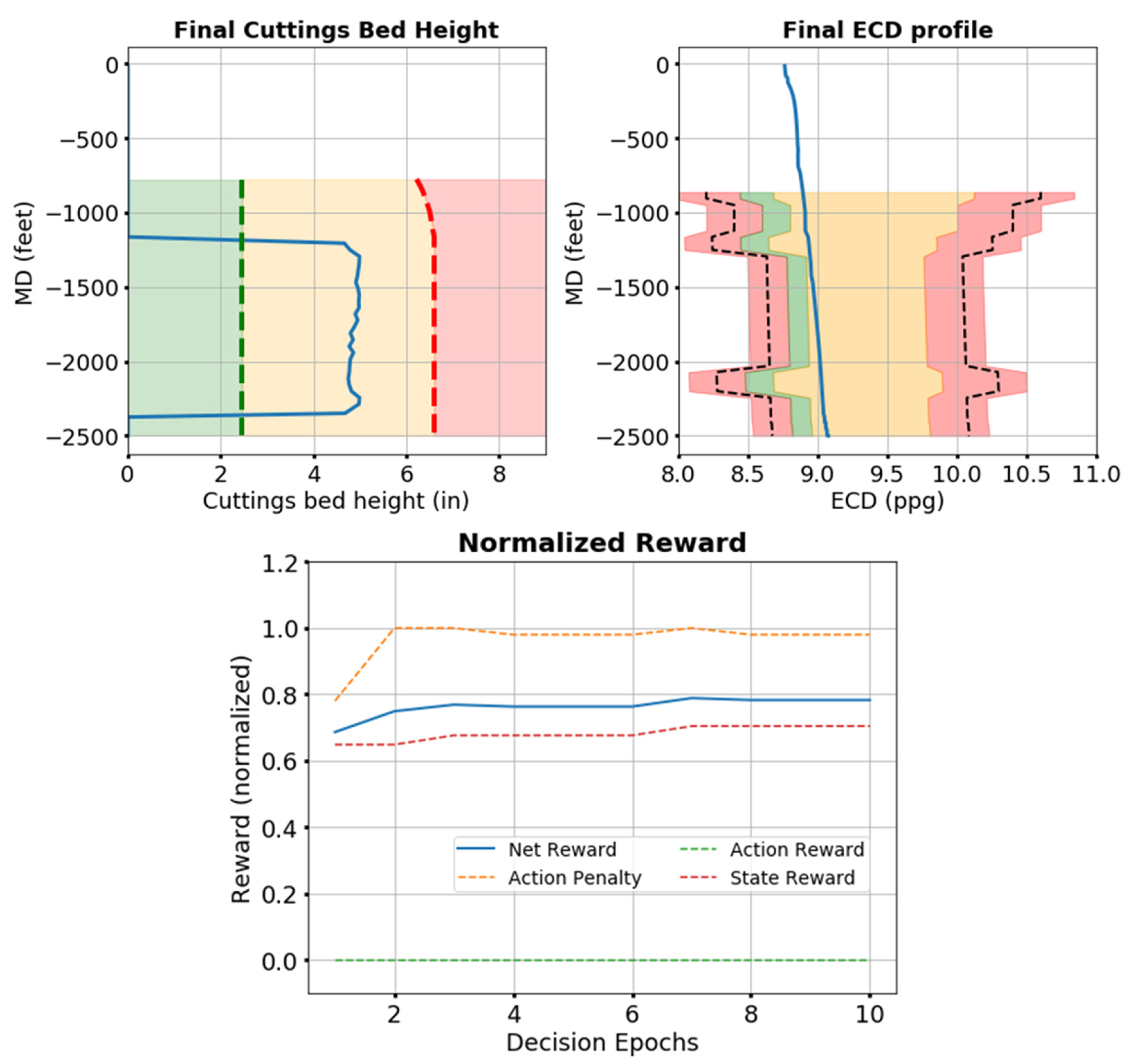
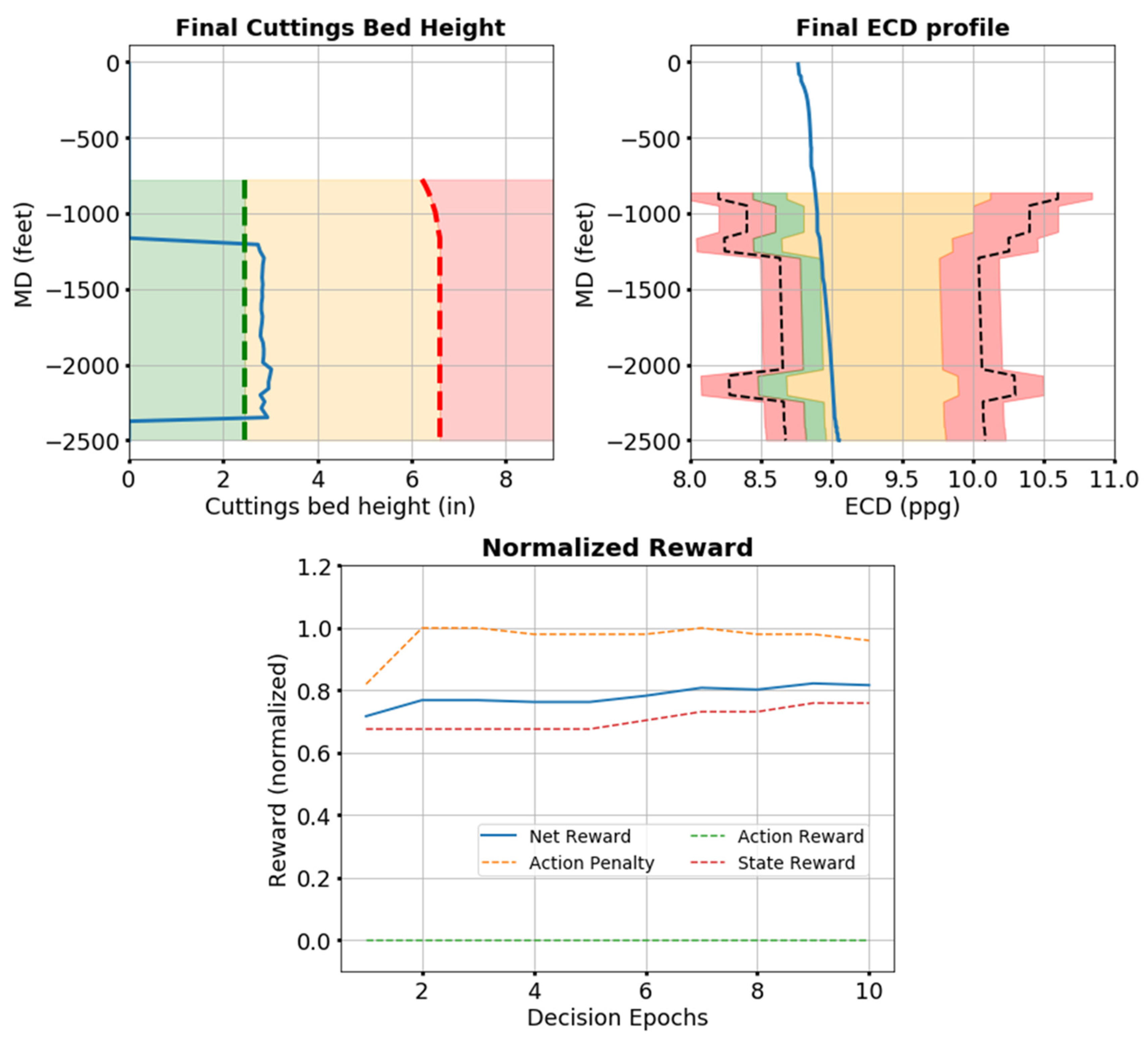
3.3.4. Calculating the Net Reward

Reward value quantifies the ‘goodness’ of taking some action from a given system state. Thus, the next step for the hole cleaning system is to combine the individual reward components to output a single reward value in the [ 0 , 1 ] range. This is accomplished by assigning different relative weights to the various components. This ability to assign different weights provides a way to prioritize different objectives. This would be advantageous in drilling wells where there is, for instance, a high risk of well control issues. In these wells, the objective of keeping the ECD within the drilling margin becomes a higher priority than completely removing the cuttings bed. Similarly, reducing the penalty associated with taking drastic actions will not be as important for certain wells as reaching the desired state quickly. Managing these objectives can be accomplished by assigning different relative weights to the individual state or action reward components.
The sets W s , W a p , and W a r , respectively, are the weights associated with sets for state transition reward, action transition penalty, and the action reward. Equations (15)–(17) represent the method for combining these weights and their associated reward sets. The final values of R S _ n e t , R a p _ n e t , and R a r _ n e t are in the ranges [ 1 , 1 ] , [ 1 , 0 ] , and [ 0 , 1 ] , respectively.
R S _ n e t = i W s i R s i i W s i
R a p _ n e t = i W a p i R a p i i W a p i
R a r _ n e t = i W a r i R a r i i W a r i
Before further combining these three components, they are first normalized to the [ 0 , 1 ] range, using the method presented in Equations (18)–(20). While this normalization is not necessary, it helps to better understand prioritization of end-user choices.
R s _ n o r m = R S _ n e t + 1 2
R a p _ n o r m = R a p _ n e t + 1
R a r _ n o r m = R a r _ n e t
Finally, the individual normalized rewards R s _ n o r m , R a p _ n o r m , and R a r _ n o r m are combined based on the weights W s _ n o r m , W a p _ n o r m , and W a r _ n o r m as per Equation (21). These weights define the relative importance of the individual normalized rewards and can also be tuned in real-time.
R n e t = W s _ n o r m R s _ n o r m + W a p _ n o r m R a p _ n o r m + W a r _ n o r m R a r _ n o r m W s _ n o r m + W a p _ n o r m + W a s _ n o r m
The above definition of the reward function ensures immediate feedback after every action, as opposed to the agent having to wait until the end of an episode (as is the case for sparse reward functions).

4. Implementation of a System as an MDP

Here, we demonstrate the developed hole cleaning decision-making system for performance tracking and action planning using a specific example. The dataset used is from an actual oil well that exhibited issues due to insufficient hole cleaning during tripping, casing, and cementing operations. This dataset included the well’s directional survey data, well profile information (casing, BHA, and bit details), one-second surface sensor data, and mud check information. A digital twin of the well was developed by integrating physics-based models (cuttings transport and hydraulics with an incorporated thermal model), data-based models (rig state detection engine), and relevant raw data sources (as detailed in Figure 9).

4.1. Well Profile

The well profile and trajectory used here are from an actual drilling operation and shown in Figure 11. The well had a short vertical section with a shallow kick-off point (where the well starts building inclination angle from vertical) around 300 feet MD. The inclination angle reached 30 degrees at approximately 750 feet MD, and 75 degrees (horizontal section) around 1250 feet MD. After this, the well remained near-horizontal until it reached its total depth (TD) of 2500 feet MD. The surface casing with an internal diameter of 13.375 inch was set at a depth of 623 feet MD. Following this, a 12.25 inch hole section was drilled to well TD. Upon reaching TD, a 50 min on-bottom circulation cycle was performed (at a flow rate of 950 gallons per minute (GPM) and 60 RPM), the drillstring was then tripped out of the hole with intermittent back-reaming (at 910 GPM and 60 RPM), and a 9.625 inch casing was run to TD and cemented.
The SL and FG values to define the drilling margins for the different sections of the well are shown in Table 3. For the near-vertical section, the SL and FG were assigned maximum values of 6 ppg and 18 ppg, respectively, because this interval was entirely cased while drilling the 12.25 inch section.
To safely run the 9.625 inch casing after drilling, calculations show that the maximum theoretical cuttings bed height (on pulling the drillstring out of hole) should not exceed approximately 5 inches (Figure 12a,b). Based on the variation in the drillstring geometry (different outer diameter and eccentric placements of various drillstring components), this bed height limit was translated into an equivalent bed height [31], assuming that the drillstring was still in the hole, with the drill bit at TD (Figure 12c). The red line in Figure 13a shows the upper limit and the green line depicts the desired limit.
Figure 13b illustrates the drilling margin limits considering an uncertainty value (DF) of ten percent. The red-colored regions in the figure correspond to intervals with potential for well control issues; the green zone, on the other hand, is the desired ECD value (goal state). The orange region is a safe but non-optimal zone. These regions correspond to the values in Table 3 with the bands corresponding to Equation (7). Similarly, in Figure 13a the red-shaded region depicts the area above the equivalent limit height, while the green-shaded region corresponds to the desired state.

4.2. Performance Tracking of the System and Summary of Issues

To track the performance of the system during drilling operations, state transitions were monitored and associated rewards were calculated. State space was defined by dividing the well into five inclination-based segments, with the procedure as discussed in the previous section. The reward function was shaped based on state and action values and transitions. Determining the action space required the specification of the discrete values of the different control variables. Table 4 shows the number and range of values for the different variables.
Table 5 shows the different weights assigned for reward calculations. For this system, the relative importance of the various state components is assumed to be the same. Similarly, relative penalties associated with altering the different action components are also assumed to be the same. Note, however, that the weights need to be determined by those who are familiar with the well, and weights used here are to provide a demonstration of the framework. The normalized reward component ( W a r _ n o r m ) has two values depending on the operation being tracked. Since no new hole is drilled during circulation operations, i.e., the ROP is zero; the weight is assigned a value of zero.
Figure 14 overlays the different normalized reward components calculated for decision epoch intervals of 5 min. For this system, the net reward tracks the state reward, since W s _ n o r m is significantly higher than the other weights. The reward value at the end of the drilling operation stabilizes to around 0.46. An increase in reward value to 0.68 at the end of the circulation cycle indicates an improvement in the hole condition. This improvement is also reflected in the state reward value, which increases from 0.51 to 0.59.
Figure 15 shows the state of the system at the end of the drilling operation (12.25 inch hole section), which can be represented by Equation (22). The mud properties for drilling the last section of the well were: mud density of 9.06 ppg, PV of 11 cP, and YP of 36.5 lbf/100 ft2. The final bed height was around 9 inches, which needed to be significantly reduced.
s T D = { 0 3 4 4 1 1 1 1 1 }
Thus, a 50 min circulation cycle to remove cuttings followed. Removal of cuttings is essential to ensure safe tripping operations without getting stuck, as well as to prepare the well for casing and cementing operations. The state of the system at the end of the circulation cycle is shown in Figure 16. As can be seen, the cuttings bed height was very close to the allowed limit, and therefore still non-optimal, leading to issues while running casing and subsequently cementing. The drilling crew did not have a process in place to evaluate various control actions; as mentioned before, this paper lays the foundational framework for that.

4.3. Basic Action Planning

Here, we discuss the utilization of the hole cleaning planning system to simulate various state–action transition options. Multiple action sequences were simulated for a 50 min (10 decision epochs) circulation interval starting from the state of well at the end of the drilling operation, s T D (represented by Equation (22)). The purpose of these simulations was to understand and quantify the effects of different action sequences on the hole condition, and in identifying a viable course of action. A viable action sequence would result in an improved wellbore condition, without compromising wellbore stability. Figure 17 details some of the simulated action sequences, where each action is structured in the form of Equation (10).
Changing the mud properties (density and rheology) is a time-consuming process; therefore, as it is highly impractical to change them in the middle of the circulation cycle, they are changed at the beginning of the action sequences. For the first four action sequences in Figure 17, PV value is increased to 21 cP, while the YP value is reduced to 21 lbf/100 ft2. For the fifth action sequence, the PV and YP are changed to 28 cP and 14 lbf/100 ft2, respectively. Finally, for the sixth sequence, PV and YP values are adjusted to 21 cP and 14 lbf/100 ft2, respectively. For the first action sequence, the mud density remains unaltered (at 9.1 ppg); for the second sequence, the density is increased to 9.4 ppg. For the remaining four action sequences, the mud density is reduced to 8.8 ppg.
Implementing action sequence number one would have resulted in a slightly better hole condition than for the actual hole after circulation, as shown in Figure 18. Note that drillstring RPM was the only parameter that was changed (from 83 to 150 RPM) in this case. The reward obtained by the system would have stabilized at around 0.76, compared with 0.68 after the circulation cycle. Additionally, the normalized state reward would have been 0.67, as compared to 0.59 after the circulation cycle (which can be seen in Figure 14).
Action sequence two would have resulted in an even lower bed height; however, the predicted ECD value at greater depths nears the upper instability region, as shown in Figure 19. In this case, only the flow rate parameter is changed (from 833 to 1500 GPM) during the operation. The expected net reward for this case would have approached 0.77, and the state reward would have stabilized around 0.69.
Figure 20 shows the predicted state after simulating action sequence number three. There would have been a significant reduction in the bed height (to approximately 4.5 inches), and the ECD value would be very close to the desired region. Both flow rate and drillstring RPM are changed during the operation; the flowrate varies from 833 to 1500 GPM, and the drillstring RPM from 83 to 150. The net and the state reward for this case would have been around 0.79 and 0.70, respectively.
Figure 21 shows the final state of the system after simulating action sequence four. The expected net and the state reward for this case would also have been around 0.79 and 0.70, respectively. As for action sequence three, both the flow rate and the drillstring RPM are increased during the operation. The primary difference between the two sequences is the order in which the changes are suggested.
The output of the execution of action sequence five is depicted in Figure 22. This sequence would result in a substantially reduced bed height (under 3.5 inches) and an ECD value very close to the desired region. The net and the state reward values for this case are 0.82 and 0.76, respectively. In this case, both the flow rate and the RPM are increased, from 833 to 1500 GPM and 83 to 150 RPM, respectively.
Figure 23 shows the expected output of implementing action sequence six. This sequence would also result in a substantially reduced bed height (under 2.5 inches) and an ECD value very close to the desired region. The expected net and state rewards would be 0.86 and 0.81, respectively, the highest among all previous simulated trajectories. In this case, both the flow rate and the RPM are increased, from 833 to 1500 GPM and 83 to 150 RPM, respectively.
This example shown on field data clearly illustrates the potential for such a decision-making approach. Explicitly classifying the hole condition (state) and quantifying state–action transitions allows the evaluation and comparison of the different action sequences, which is a vital component in building an intelligent hole cleaning advisory system. Table 6 summarizes the net and the state rewards associated with the different action sequences. Here, action sequence number six has the best performance (as quantified by the highest final state reward) and also has the highest net reward (which depends on both the final state and the state–action transitions).

5. Conclusions

This paper proposes and justifies setting up well construction operations as finite–horizon sequential decision-making systems for long-term planning. To the best of our knowledge, this is the first time a well construction operation has been structured as an MDP with carefully shaped rewards and an integrated multi-model digital twin, and subsequently utilized for evaluating action sequences. Such representation of well construction operations allows for an unbiased quantification and comparison of different scenarios. To summarize, this paper:
-
Discusses the requirements and the steps in setting up such systems (i.e., formulating an MDP, defining the goal state, efficient reward shaping, and digitally twinning the underlying process) by detailing the development of a hole cleaning decision-making system.
-
Discusses the importance of reward shaping for well construction operations to ensure frequent and suitable feedback, thereby facilitating effective policy design. It also demonstrates the use of a non-sparse normalized reward function designed for a hole cleaning system for performance tracking and simple action planning.
-
Demonstrates the use of digital twinning for simulating various action sequences to track the state evolution and reward progression, thereby allowing ranking of the different sequences based on their long-term returns.
Furthermore, more directed search and planning methods such as simulation-based search can be deployed on these systems to enhance system performance considerably. In the longer-term, such decision engines can be incorporated into a rig’s control system to help automate control of action variables such as RPM, flowrate, tripping speeds, and mud rheology. This will thereby enable the full automation of complex drilling operations such as hole cleaning. This, in turn, will avoid any human-centric biases and eliminate human mistakes in well construction operations and their negative consequences, such as stuck pipe incidents, induced well control and lost circulation incidents, etc. The outlined approach is therefore expected to have a potentially large positive impact on the efficiency, economics, and safety of future well construction operations.

Author Contributions

Conceptualization, G.S.S., P.A. and E.v.O.; methodology, G.S.S., O.E., P.A. and E.v.O.; software, G.S.S. and O.E.; validation, G.S.S., O.E. and P.A.; formal analysis, G.S.S.; investigation, G.S.S. and O.E.; resources, P.A. and E.v.O.; data curation, G.S.S. and P.A.; writing—original draft preparation, G.S.S.; writing—review and editing, O.E., P.A. and E.v.O.; visualization, G.S.S.; supervision, P.A. and E.v.O.; project administration, E.v.O.; funding acquisition, P.A. and E.v.O. All authors have read and agreed to the published version of the manuscript.

Funding

Funding was provided by the RAPID Industry Affiliate Program (IAP) at the University of Texas at Austin.

Acknowledgments

The authors would like to thank the members of the Rig Automation and Performance Improvement in Drilling (RAPID) consortium at the University of Texas at Austin for their support of this research. We would also like to acknowledge our colleagues in the research group for valuable brainstorming sessions.

Conflicts of Interest

The authors declare no conflict of interest.

Glossary

Unit conversion
1 m (m)3.28 feet (ft)
1 meter/second (m/s)11811 feet/hour (ft/hr.)
1 psi6894.76 Pa
1 ppg119.83 kg/m3
1 radian57.2958 degrees
1 ft30.02832 m3
1 GPM0.0000631 m3/s
1 cP0.001 Pa·s
1 lb./100ft20.4788 Pa
1 lbs.0.4536 Kg
Nomenclature
A Action space
a t Action executed by the agent at time t
D o _ k Outer diameter of the kth control volume segment (inches)
D T V D Total vertical depth (m)
E C D Equivalent circulation density (pounds per gallon or ppg)
E C D k a b s o l u t e Absolute ECD value in the kth control volume segment (ppg)
E C D a v g The average ECD value for an inclination interval (ppg)
E C D i n c . Functional value of ECD in the inclination interval segment i n c .
F G Fracture gradient (ppg)
f l o w r a t e Rate of flow of the drilling mud through the drillstring controlled by a positive displacement reciprocating mud pump on the surface (GPM)
G P M Gallons per minute
g Acceleration due to gravity (9.81 m/s2)
H Normalized cuttings bed height for an inclination interval
H i n c . Functional value of the cuttings bed height in the inclination interval segment i n c l .
H k a b s o l u t e Absolute cuttings bed height in the kth control volume segment (inches)
H k n o r m Normalized cuttings bed height in the kth control volume segment
i n c l 
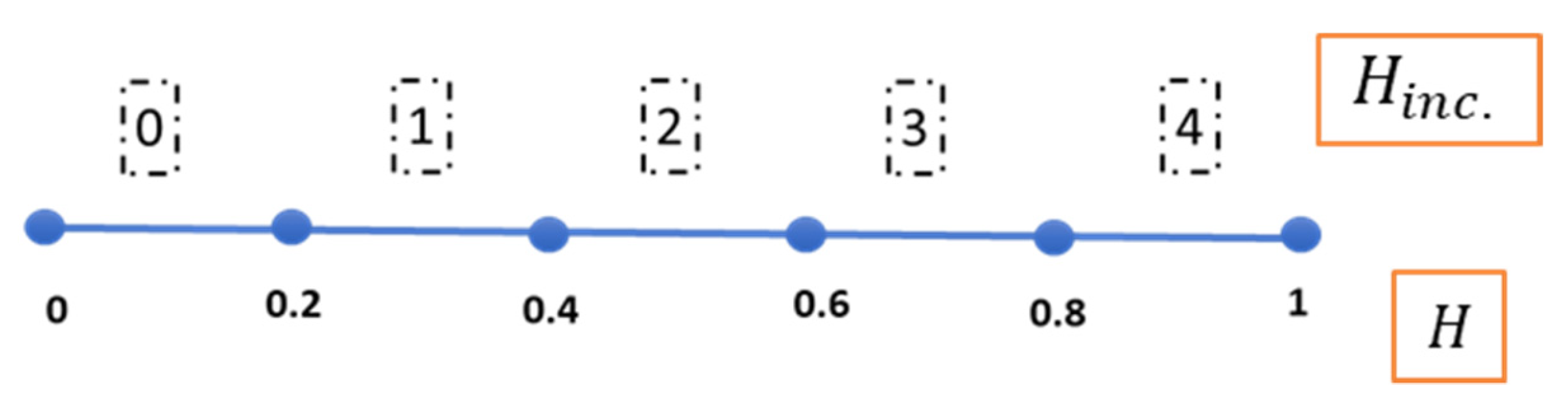
Inclination angle range (degrees)
N s e g Number of control volume segments within an inclination interval segment
n i n t e r v a l Number of discrete values possible for a given control variable
P Transition probability set
P f r i c t i o n a l p r e s s u r e _ l o s s _ D M D Frictional pressure drop in the annulus (Pa) at a measured depth H
P h y d r o s t a t i c _ D T V D Hydrostatic pressure (Pa) at a vertical depth of TVDH
P s s a Transition probability of a system in the state s to the state s when an agent executes action a
P V Plastic viscosity (cP)
p i ith parameter component of the state vector
p g i Goal state value of the ith parameter component of the state vector
R Reward set
R a p Action transition-based penalty set
R a p _ n e t Non-normalized action penalty for the hole cleaning system
R a p _ n o r m Normalized action penalty for the hole cleaning system
R a r Action value-based reward set
R a r _ n e t Non-normalized action reward for the hole cleaning system
R a r _ n o r m Normalized action reward for the hole cleaning system
R n e t Net normalized reward function for the hole cleaning system
R S State transition-based reward set
R S _ n e t Non-normalized state reward for the hole cleaning system
R s _ n o r m Normalized state reward for the hole cleaning system
R O P Rate of penetration or drilling rate (ft/hr.)
R P M Drillstring rotation speed (revs. /min)
r t Reward received by the system at time t
S State space
S L Stability limit (ppg)
s g o a l Goal or desired state for the hole cleaning system
s t State of the system at time t
s T D State of the hole cleaning system at the well TD
T D Total depth of the well (feet)
t Time step or decision epoch   t
W a p Weight set associated with the action transition penalty
W a p _ n o r m Weight value associated with the normalized action penalty
W a r Weight set associated with the action value reward
W a r _ n o r m Weight value associated with the normalized action reward
W s Weight set associated with state transition reward
W s _ n o r m Weight value associated with the normalized state reward
W O B Weight on bit (Klbs.)
Y P Yield point (lb./100ft2)
Δ N v a r i a b l e Number of interval changes between consecutive actions
Δ w Difference between the FG and SL of the drilling window (ppg)
π Policy
γ Discount factor for return calculation

References

  1. Gholami Mayani, M.; Rommetveit, R.; Oedegaard, S.I.; Svendsen, M. Drilling automated realtime monitoring using digital twin. In Proceedings of the Abu Dhabi International Petroleum Exhibition & Conference, Abu Dhabi, United Arab Emirates, 12–15 November 2018. [Google Scholar] [CrossRef]
  2. Chan, H.C.; Lee, M.M.; Saini, G.S.; Pryor, M.; van Oort, E. Development and Validation of a Scenario-Based Drilling Simulator for Training and Evaluating Human Factors. IEEE Trans. Hum.-Mach. Syst. 2020, 50, 327–336. [Google Scholar] [CrossRef]
  3. Ahmed, O.S.; Aman, B.M.; Zahrani, M.A.; Ajikobi, F.I.; Aramco, S. Stuck Pipe Early Warning System Utilizing Moving Window Machine Learning Approach. In Proceedings of the Abu Dhabi International Petroleum Exhibition & Conference, Abu Dhabi, United Arab Emirates, 11–14 November 2019. [Google Scholar] [CrossRef]
  4. Forshaw, M.; Becker, G.; Jena, S.; Linke, C.; Hummes, O. Automated hole cleaning monitoring: A modern holistic approach for NPT reduction. In Proceedings of the International Petroleum Technology Conference 2020, IPTC 2020, Dammam, Saudi Arabia, 13–15 January 2020. [Google Scholar] [CrossRef]
  5. Erge, O.; van Oort, E. Time-dependent cuttings transport modeling considering the effects of eccentricity, rotation and partial blockage in wellbore annuli. J. Nat. Gas Sci. Eng. 2020, 82, 103488. [Google Scholar] [CrossRef]
  6. Kunath, M.; Winkler, H. Integrating the Digital Twin of the manufacturing system into a decision support system for improving the order management process. Procedia CIRP 2018, 72, 225–231. [Google Scholar] [CrossRef]
  7. Kiran, B.R.; Sobh, I.; Talpaert, V.; Mannion, P.; Al Sallab, A.A.; Yogamani, S.; Pérez, P. Deep reinforcement learning for autonomous driving: A survey. IEEE Trans. Intell. Transp. Syst. 2021, 23, 4909–4926. [Google Scholar] [CrossRef]
  8. Schwarting, W.; Alonso-Mora, J.; Rus, D. Planning and Decision-Making for Autonomous Vehicles. Annu. Rev. Control Robot. Auton. Syst. 2018, 1, 187–210. [Google Scholar] [CrossRef]
  9. Kang, D.-J.; Park, J.H.; Yeo, S.-S. Intelligent Decision-Making System with Green Pervasive Computing for Renewable Energy Business in Electricity Markets on Smart Grid. EURASIP J. Wirel. Commun. Netw. 2009, 2009, 1. [Google Scholar] [CrossRef] [Green Version]
  10. Olaf Blech, J.; Fernando, L.; Foster, K. Towards Decision Support for Smart Energy Systems based on Spatio-temporal Models. arXiv 2017, arXiv:1705.03860. [Google Scholar]
  11. Silver, D.; Schrittwieser, J.; Simonyan, K.; Antonoglou, I.; Huang, A.; Guez, A.; Hubert, T.; Baker, L.; Lai, M.; Bolton, A.; et al. Mastering the game of Go without human knowledge. Nature 2017, 550, 354–359. [Google Scholar] [CrossRef] [PubMed]
  12. Silver, D.; Hubert, T.; Schrittwieser, J.; Antonoglou, I.; Lai, M.; Guez, A.; Lanctot, M.; Sifre, L.; Kumaran, D.; Graepel, T.; et al. A general reinforcement learning algorithm that masters chess, shogi, and Go through self-play. Science 2018, 362, 1140–1144. [Google Scholar] [CrossRef] [PubMed] [Green Version]
  13. Arulkumaran, K.; Cully, A.; Togelius, J. AlphaStar: An Evolutionary Computation Perspective. In Proceedings of the Genetic and Evolutionary Computation Conference Companion, Prague, Czech Republic, 13–17 July 2019; pp. 314–315. [Google Scholar] [CrossRef] [Green Version]
  14. OpenAI Five. 2018. Available online: https://openai.com/blog/openai-five/ (accessed on 1 July 2020).
  15. LaValle, S.M. Planning Algorithms; Cambridge University Press: Cambridge, UK, 2006. [Google Scholar] [CrossRef] [Green Version]
  16. Poole, D.L.; Mackworth, A.K. Artificial Intelligence: Foundations of Computational Agents, 2nd ed.; Cambridge University Press: Cambridge, UK, 2017. [Google Scholar]
  17. Vodopivec, T.; Samothrakis, S.; Ŝter, B. On Monte Carlo Tree Search and Reinforcement Learning. J. Artif. Intell. Res. 2017, 60, 881–936. [Google Scholar] [CrossRef]
  18. Saini, G.S. Digital Twinning of Well Construction Operations for Improved Decision-Making. Ph.D. Thesis, The University of Texas at Austin, Austin, TX, USA, 2020. [Google Scholar]
  19. Silver, D.; Sutton, R.S.; Müller, M. Temporal-difference search in computer Go. Mach. Learn. 2012, 87, 183–219. [Google Scholar] [CrossRef] [Green Version]
  20. Sutton, R.S.; Barto, A.G. Reinforcement Learning: An Introduction, 2nd ed.; The MIT Press: Cambridge, MA, USA, 2018. [Google Scholar]
  21. Puterman, M.L. (Ed.) Markov Decision Processes; John Wiley & Sons, Inc.: Hoboken, NJ, USA, 1994. [Google Scholar] [CrossRef] [Green Version]
  22. Cochran, J.J.; Cox, L.A., Jr.; Keskinocak, P.; Kharoufeh, J.P.; Smith, J.C.; Feinberg, E.A. Total Expected Discounted Reward MDPS: Existence of Optimal Policies. In Encyclopedia of Operations Research and Management Science; Cochran, J.J., Cox, L.A., Keskinocak, P., Kharoufeh, J.P., Smith, J.C., Eds.; Wiley: New York, NY, USA, 2011. [Google Scholar] [CrossRef] [Green Version]
  23. Wiewiora, E. Reward Shaping. In Encyclopedia of Machine Learning and Data Mining; Springer: Berlin/Heidelberg, Germany, 2017; pp. 1104–1106. [Google Scholar] [CrossRef]
  24. Jones, D.; Snider, C.; Nassehi, A.; Yon, J.; Hicks, B. Characterising the Digital Twin: A systematic literature review. CIRP J. Manuf. Sci. Technol. 2020, 29, 36–52. [Google Scholar] [CrossRef]
  25. Saini, G.S.; Ashok, P.; van Oort, E. Predictive action planning for hole cleaning optimization and stuck pipe prevention using digital twinning and reinforcement learning. In Proceedings of the SPE/IADC Drilling Conference, Houston, TX, USA, 3 March 2020. [Google Scholar] [CrossRef]
  26. Mitchell, R.F.; Miska, S.Z.; Cunha, J.; Kastor, R.; Aadnoy, B.S.; Eustes, I.A.; Sweatman, R.; Kelessidis, V.C.; Maglione, R.; Ozbayoglu, E.; et al. Fundamentals of Drilling Engineering; Society of Petroleum Engineers: Richardson, TX, USA, 2011. [Google Scholar]
  27. Bourgoyne, A.T. Applied Drilling Engineering; Society of Petroleum Engineers: Richardson, TX, USA, 1986. [Google Scholar]
  28. Sanchez, R.A.; Azar, J.J.; Bassal, A.A.; Martins, A.L. The Effect of Drillpipe Rotation on Hole Cleaning During Directional Well Drilling. In Proceedings of the SPE/IADC Drilling Conference, Amsterdam, The Netherlands, 4 April 1997. [Google Scholar] [CrossRef]
  29. Sifferman, T.R.; Becker, T.E. Hole cleaning in full-scale inclined wellbores. SPE Drill. Eng. 1992, 7, 115–120. [Google Scholar] [CrossRef]
  30. Baldino, S.; Osgouei, R.E.; Ozbayoglu, E.; Miska, S.; Takach, N.; May, R.; Clapper, D. Cuttings settling and slip velocity evaluation in synthetic drilling fluids. In Proceedings of the Offshore Mediterranean Conference and Exhibition, OMC, Ravenna, Italy, 25 March 2015. [Google Scholar]
  31. Cayeux, E.; Mesagan, T.; Tanripada, S.; Zidan, M.; Fjelde, K.K. Real-time evaluation of hole-cleaning conditions with a transient cuttings-transport model. SPE Drill. Completion 2014, 29, 5–21. [Google Scholar] [CrossRef]
  32. Erge, O.; Ozbayoglu, E.M.; Miska, S.Z.; Yu, M.; Takach, N.; Saasen, A.; May, R. The effects of drillstring-eccentricity, -rotation, and -buckling configurations on annular frictional pressure losses while circulating yield-power-law fluids. SPE Drill. Completion 2015, 30, 257–271. [Google Scholar] [CrossRef]
  33. Gul, S.; van Oort, E.; Mullin, C.; Ladendorf, D. Automated Surface Measurements of Drilling Fluid Properties: Field Application in the Permian Basin. SPE Drill. Completion 2020, 35, 525–534. [Google Scholar] [CrossRef]
  34. Saasen, A.; Løklingholm, G. The Effect of Drilling Fluid Rheological Properties on Hole Cleaning. In Proceedings of the IADC/SPE Drilling Conference, Dallas, TX, USA, 4 April 2002. [Google Scholar] [CrossRef]
  35. Nazari, T.; Hareland, G.; Azar, J.J. Review of Cuttings Transport in Directional Well Drilling: Systematic Approach. In Proceedings of the SPE Western Regional Meeting, Anaheim, CA, USA, 27–29 May 2010. [Google Scholar] [CrossRef]
  36. Karstad, E.; Aadnoy, B.S. Analysis of temperature measurements during drilling. In Proceedings of the SPE Annual Technical Conference and Exhibition, San Antonio, TX, USA, 5–8 October 1997. [Google Scholar] [CrossRef]
  37. Bassal, A.A. The Effect of Drillpipe Rotation on Cuttings Transport in Inclined Wellbores. Ph.D. Thesis, University of Tulsa, Tulsa, OK, USA, 1995. [Google Scholar]
  38. Duan, M.; Miska, S.; Yu, M.; Takach, N.; Ahmed, R.; Zettner, C. Critical conditions for effective sand-sized solids transport in horizontal and high-angle wells. SPE Drill. Completion 2009, 24, 229–238. [Google Scholar] [CrossRef]
  39. Jalukar, L.S. A Study of Hole Size Effect on Critical and Subcritical Drilling Fluid Velocities in Cuttings Transport for Inclined Wellbores. Ph.D. Thesis, University of Tulsa, Tulsa, OK, USA, 1993. [Google Scholar]
  40. Larsen, T.I.; Pilehvari, A.A.; Azar, J.J. Development of a new cuttings-transport model for high-angle wellbores including horizontal wells. SPE Drill. Completion 1997, 12, 129–135. [Google Scholar] [CrossRef]
  41. Larsen, T.I.F. A Study of the Critical Fluid Velocity in Cuttings Transport for Inclined Wellbores. Ph.D. Thesis, University of Tulsa, Tulsa, OK, USA, 1990. [Google Scholar]
  42. Naganawa, S.; Nomura, T. Simulating transient behavior of cuttings transport over whole trajectory of extended reach well. In Proceedings of the IADC/SPE Asia Pacific Drilling Technology Conference and Exhibition, Bangkok, Thailand, 11–13 October 2006. [Google Scholar] [CrossRef]
  43. Rubiandini, R.S. Equation for estimating mud minimum rate for cuttings transport in an inclined-until-horizontal well. In Proceedings of the SPE/IADC Middle East Drilling Technology Conference, Abu Dhabi, United Arab Emirates, 8 November 1999. [Google Scholar] [CrossRef]
Figure 1. Agent–environment interaction in RL (modified from [20]).
Energies 15 05776 g001
Figure 2. The proposed strategy for defining discrete state spaces based on wellbore inclination angles.
Energies 15 05776 g002
Figure 3. Application of MDP and digital twins for simulating episodes to determine the optimal policy.
Energies 15 05776 g003
Figure 4. (a) Drilling safety margin; (b) Cuttings bed distribution in different inclination segments of the well.
Energies 15 05776 g004
Figure 5. Absolute cuttings bed height for a single control volume element.
Energies 15 05776 g005
Figure 6. Functional value assignment for the cuttings bed height parameter.
Energies 15 05776 g006
Figure 7. Functional value assignment for the ECD parameter.
Energies 15 05776 g007
Figure 8. Variables contributing to the hole cleaning performance in a deviated hole (modified from [35]).
Energies 15 05776 g008
Figure 9. Digital twin of the hole cleaning system’s environment (see [18] for details on the models).
Energies 15 05776 g009
Figure 10. Example calculation of an action transition-based penalty and reward associated with action.
Energies 15 05776 g010
Figure 11. Well trajectory and inclination profile (negative sign indicates downward depth into the sub-surface).
Energies 15 05776 g011
Figure 12. The theoretical limit of allowed cuttings bed height for the given well profile. (c) Equations in [31].
Energies 15 05776 g012
Figure 13. (a) Limits of the cuttings bed height profile. (b)The drilling margin for the well considering a ten percent uncertainty in the SL and FG limits (negative sign indicates downward depth into the sub-surface).
Energies 15 05776 g013
Figure 14. Normalized reward components versus decision epochs for the well.
Energies 15 05776 g014
Figure 15. State of the borehole at the end of the drilling operation.
Energies 15 05776 g015
Figure 16. State of the borehole at the end of the circulation cycle.
Energies 15 05776 g016
Figure 17. Six action sequences simulated in this work and discussed in detail in the text.
Energies 15 05776 g017
Figure 18. Predicted final system state and rewards after implementing action sequence one.
Energies 15 05776 g018
Figure 19. Predicted final system state and rewards after implementing action sequence two.
Energies 15 05776 g019
Figure 20. Predicted final system state and rewards after implementing action sequence three.
Energies 15 05776 g020
Figure 21. Predicted final system state and rewards after implementing action sequence four.
Energies 15 05776 g021
Figure 22. Predicted final system state and rewards after implementing action sequence five.
Energies 15 05776 g022
Figure 23. Predicted final system state and rewards after implementing action sequence six.
Energies 15 05776 g023
Table 1. Reward function associated with state vector components.
ComponentReward FunctionValues
H 30 45 R H 30 45 = 2 H 30 45 2 { 1 ,   0.33 , 0.33 , 1 }
H 45 60 R H 45 60 = 2 H 45 60 2 { 1 ,   0.33 , 0.33 , 1 }
H 60 75 R H 60 75 = 2 H 60 75 2 { 1 ,   0.33 , 0.33 , 1 }
H 75 + R H 75 + = 2 H 75 + 2 { 1 ,   0.33 , 0.33 , 1 }
ECD 0 30 R ECD 0 30 = 1 2 3 · | E 0 30 | { 1 , 0.33   ,   0.33   ,   1   ,   0.33   , 0.33   , 1 }
ECD 30 45 R ECD 30 45 = 1 2 3 · | E 30 45 | { 1 , 0.33   ,   0.33   ,   1   ,   0.33   , 0.33   , 1 }
ECD 45 60 R ECD 45 60 = 1 2 3 · | E 45 60 | { 1 , 0.33   ,   0.33   ,   1   ,   0.33   , 0.33   , 1 }
ECD 60 75 R ECD 60 75 = 1 2 3 · | E 60 75 | { 1 , 0.33   ,   0.33   ,   1   ,   0.33   , 0.33   , 1 }
ECD 75 + R ECD 75 + = 1 2 3 · | E 75 + | { 1 , 0.33   ,   0.33   ,   1   ,   0.33   , 0.33   , 1 }
Table 2. Reward function associated with action transition.
ComponentNo. of Intervals Reward FunctionValues
F l o w r a t e n f l o w r a t e R f l o w r a t e = | Δ N f l o w r a t e | n f l o w r a t e [ 1 ,   0 ]
D r i l l i n g   R O P n R O P R R O P = | Δ N R O P | n R O P [ 1 ,   0 ]
D r i l l s t r i n g   R P M n R P M R R P M = | Δ N R P M | n R P M [ 1 ,   0 ]
M u d   d e n s i t y   n d e n s i t y R d e n s i t y = | Δ N d e n s i t y | n d e n s i t y   [ 1 ,   0 ]
M u d   P V n P V R P V = | Δ N P V | n P V [ 1 ,   0 ]
M u d   Y P n Y P R Y P = | Δ N Y P | n Y P [ 1 ,   0 ]
Table 3. The SL and FG values to define drilling margin for the different inclination intervals.
Inclination IntervalStability Limit (ppg)Fracture Gradient (ppg)
[0, 30)—in casing618
[30, 45)8.210.6
[45, 60)8.410.4
[60, 75)8.210.2
[75+)8.610.0
Table 4. Value discretization of control variables.
Control VariableNumber of Discrete ValuesRange of Values
Flow Rate (GPM)10[0, 1500]
Drilling ROP (ft/h)10[0, 900]
Drillstring RPM (rev/min)10[0, 150]
Mud Density (ppg)5[8.5, 9.7]
Mud Plastic Viscosity (cP) 5[7, 42]
Mud Yield Point (lb./100ft2)5[7, 42]
Table 5. Weight assignments for reward function shaping.
W s = [ 1 ,   1 ,   1 ,   1 ,   1 ,   1 ,   1 ,   1 ,   1 ]
W a p = [ 1 ,   1 ,   1 ,   1 ,   1 ,   1 ]
W a r = [ 0 ,   1 ,   0 ,   0 ,   0 ,   0 ]
W s _ n o r m = 0.50
W a p _ n o r m = 0.20
DrillingCirculation
W a r _ n o r m = 0.30 W a r _ n o r m = 0.00
Table 6. Summary of the rewards associated with the different action sequences.
Action SequenceNet RewardFinal State Reward
0 (Original)0.680.59
10.760.68
20.770.69
30.790.70
40.790.70
50.820.76
60.860.81
Publisher’s Note: MDPI stays neutral with regard to jurisdictional claims in published maps and institutional affiliations.

