A Heat Exchanger with Water Vapor Condensation on the External Surface of a Vertical Pipe

Abstract

The paper is concerned with water vapor condensation on vertical pipes. The vertical position of pipes in a condenser is not discussed very often. Its application has a number of particularities in terms of the numerical determination of heat transfer. In the first stage of this paper, the authors focus on the experimental identification of heat transfer during vapor condensation on vertical pipes with a diameter of 14.0 × 1.0 mm. The pipes are placed in a narrow channel and the steam flows around them in a perpendicular direction. Two channel widths were tested, i.e., 20.0 and 24.0 mm. In the second stage, numerical modelling (CFD) is used for a detailed identification of the vapor velocity fields near the pipes. In the third stage, the results of the experimental measurements and numerical modelling are compared with data published by various authors. There are studies in the literature dealing with axial flow around vertical pipes; however, the associated results are based on conditions which are distinct from those applied in our study. The outcome of this paper is the specification of the heat transfer coefficient and the calculation formulas precisely describing the studied condenser configuration.

1. Introduction

Vapor condensation is a physical process used in many practical applications such as the cooling systems of thermal or nuclear power plants, air conditioning units and other heat exchange equipment [1]. Condensation can be defined as a phase change of a substance from a gaseous to a liquid state. During this change, a large amount of energy is released in the form of latent heat. The condensation process is very intense at the vapor–liquid phase interface. The width of this interface ranges from 1 to 2 molecule diameters [2].

The first detailed description of condensation was provided by Wilhelm Nusselt in his publication [3] in 1916, where he explained the gravitational principle of laminar film condensation. Nusselt’s description was later modified by Sparrow [4], who took into consideration the influence of a change in the momentum of the condensate on a vertical surface due to gravity. Later, the character of the condensate film flow (laminar, turbulent) started to be distinguished and the influence of shear stress in the gaseous phase on the liquid interface was included, which causes deformation of the film and undulation of its surface. This was mathematically described by, for example, Aktershev, who examined [5] the influence of flowing gas on liquid films for both concurrent and counter-current arrangements. In [6], Aktershev used the finite element method to describe the formation of natural waves and identified the areas where the condensate film starts to be unstable.

A literature survey revealed a considerable discrepancy between the number of studies on water vapor condensation inside a vertical pipe and research on condensation on the external side of vertical pipes. It is almost impossible to find relevant studies on this topic before 1980. What can be mentioned is, for example, a publication by Jacobs [7] which showed that the inertia components of a liquid film have an insignificant influence, and that the distribution of temperature across the film is linear.

In their publication [8], Fujii and Uehara dealt with the theory of a two-phase interface for laminar membrane condensation according to Jacobs on the external surface. They also proposed formulas for calculating the local Nusselt number. Winkler and Chen studied the condensation of saturated and superheated vapor along an isothermal vertical board in modes with the predominance of forced and free convection. The authors came to the conclusion that the buoyancy force generated during condensation at the interface considerably increases the shear stress and, to a lesser extent, also increases the heat flux of the walls. Superheating pure vapor only causes a negligible increase in the heat flux of the walls [9]. Their work formed the basis for Zhao et al. and their publication [10] investigating the condensation of R134a coolant and the effects of superheating the coolant on the condensation process. It emerged that a combination of convection and condensation during vapor superheating decreases the condensation heat transfer. Chang [11] analysed steady mixed convection of a condensate film running along an isothermal vertical pipe in dry saturated vapor with forced flow. The results showed that the common assumption of zero interface shear stress was not applicable to the case of forced vapor flow. Tong et al. tested condensation on a vertical smooth pin-fin pipe with free convection. The experiment showed better efficiency of the pin-fin pipe. The efficiency grew with greater undercooling of the wall and with an increasing content of air in the water vapor [12]. This work was followed up by Guangming et al. [13], who examined the difference between condensation on a smooth and corrugated pipe. The result of the output measurement showed that the difference in the heat transfer characteristics on the crest and trough was not significant but, for pure vapor, the heat transfer coefficient for the corrugated pipe was 10% greater than that for the smooth pipe. Studies of condensation on the external side of a vertical pipe tested the states of stationary or slightly moving vapor.

This paper focuses on condensation on the external side of vertical pipes placed in a narrow channel of a heat exchanger, where saturated vapor runs at an increased speed against the pipes from the side, i.e., in a cross-like arrangement. The results will be compared with the analytical relationships presented in the studies mentioned above describing the condensation of stationary vapor on the external surface of vertical pipes.

2. Experiment

As part of this study, experiments were conducted to identify the heat flux and condensation heat transfer coefficients on the external side of three vertical pipes inside a narrow rectangular channel for different mass flow rates and, thus, different velocities of vapor flow around a row of pipes.

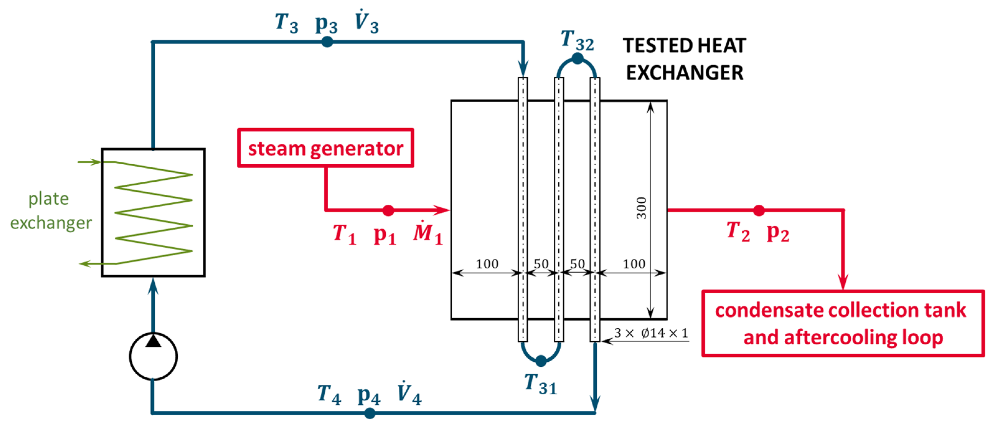
2.1. Experimental Device

The testing section of the heat exchanger had a size of 300 × 300 mm and the basic width of the flow channel in free space was 24 mm. In the reduced version of the flow channel, the width was 20 mm. The exchanger was insulated with fiberglass to prevent heat loss to the surroundings. The channel contained three stainless steel pipes with outer diameters of 14.0 mm and wall thicknesses of 1.0 mm. The basic geometric dimensions are shown in Figure 1 in a simplified diagram of the experimental device. Cooling water ran inside the pipes and entered the upper part of the first pipe at the required temperature, pressure, and flow rate ($T_3$, ${\mathrm{p}}_3$ and ${\dot{V}}_3$). The cooling water exited the lower part of the first pipe with a measured temperature of $T_{31}$ and was led into the lower part of the second pipe. The cooling water exited the upper part of the second pipe with a measured temperature of $T_{32}$ and entered the upper part of the third pipe. The cooling water exited the third pipe with a measured temperature and pressure of ($T_4$, ${\mathrm{p}}_4$). The cooling water ran in a closed loop, where there were, among other things, a circulation pump controlled by a frequency convertor and two plate exchangers transferring heat and controlling the cooling water temperature at the inlet into the testing section ($T_3$).

Saturated water vapor was brought into the testing section from a steam generator. It was possible to adjust the amount and temperature (pressure) of the steam being generated since the steam generator also included a steam superheater (up to 700 °C), although this was not used in the experiments. The vapor parameters measured at the inlet into the testing section included temperature, pressure, and flow rate ($T_1$, ${\mathrm{p}}_1$ and ${\dot{M}}_1$). Condensate with a measured temperature and pressure of $T_2$, ${\mathrm{p}}_2$ was removed from the testing section, together with non-condensed vapor, and taken into a condensate collection tank, which also included an aftercooling loop.

The temperature at the key nodes of the experimental device (points 1, 2, 3 and 4) was measured in two ways. The first (1) used type-T thermocouples, coated and ungrounded, while the other one (2) used resistance temperature sensors (PT100). At points 31 and 32, only the thermocouples of the type already mentioned were used. The pressure of the water/water vapor was measured by the PXM 319 and Baumer TED6 pressure sensors. The cooling water flow rate was measured by the Flomag 3000 induction flowmeter with a convertor.

2.2. Analytical Model

To determine the condensation heat transfer coefficient on a pipe, we must know the total heat transfer coefficient. This depends on the material and thickness of the pipe wall and, primarily, on the intensity of the power transmitted. Due to the insulation of the heat exchanger, the loss to the surroundings may be omitted. Not considering the heat loss to the surroundings, the heat transferred on the vapor side must be equal to the heat absorbed by the cooling water, based on the following relation

$${\dot{Q}}_{12}={\dot{Q}}_{34}⟺{\dot{Q}}_1-{\dot{Q}}_2={\dot{Q}}_4-{\dot{Q}}_3 \left[\mathrm{W}\right],$$

(1)

where ${\dot{Q}}_{34}$ is the cooling power, which is a function of the flow rate, pressure and the input and output temperature of the cooling water

$${\dot{Q}}_{34}={\dot{V}}_3·\rho \left(\frac{p_3+p_4}{2};\frac{t_3+t_4}{2}\right)·c_p\left(\frac{p_3+p_4}{2};\frac{t_3+t_4}{2}\right)·\left(t_4-t_3\right) \left[\mathrm{W}\right].$$

(2)

Heat transferred on the side of the vapor can be latent heat, released during the water vapor condensation, or sensible heat, generated by the condensate film cooling down on the pipes. In comparison with latent heat, sensible heat is negligible. The total amount of condensed vapor can then be calculated from the power produced and the latent heat of the phase transformation for the given temperatures according to Equation (3). The amount of condensate generated on each pipe can then be determined by substituting the proper variables into this equation.

$${\dot{M}}_{2k}=\frac{{\dot{Q}}_{34}}{i\left(p_{12};t_1\right)-i\left(p_{12};t_2\right)} \left[\mathrm{kg}·{\mathrm{s}}^{-1}\right],$$

(3)

The heat transfer from the condensing vapor into the pipe wall consists of convective heat transfer and conduction. Considering the temperatures of the vapor and the condensate, the radiation heat can be omitted. The total heat transfer coefficient is then given by Equation [14].

$$k_S=\frac{{\dot{Q}}_{34}}{n·L·\mathsf{\Delta }{T}_{ln}} \left[\mathrm{W}·{\mathrm{m}}^{-1}·{\mathrm{K}}^{-1}\right],$$

(4)

where $n$ is the number of pipes, $L \left[\mathrm{m}\right]$ is the length of one pipe and $\mathsf{\Delta }{T}_{ln} \left[°\mathrm{C}\right]$ is the logarithmic temperature gradient, which can be determined for the concurrent arrangement of the exchanger as follows

$$\mathsf{\Delta }{T}_{ln}=\frac{\left(t_1-t_3\right)-\left(t_2-t_4\right)}{\ln \left(\frac{t_1-t_3}{t_2-t_4}\right)} \left[°\mathrm{C}\right].$$

(5)

The calculation of the logarithmic temperature gradient in a concurrent arrangement can be applied to the exchanger as a whole (all three rows) or separately to the first and third row. When doing the calculation separately only for the second row, it is a counter current arrangement, and the logarithmic temperature gradient is

$$\mathsf{\Delta }{T}_{ln}=\frac{\left(t_1-t_4\right)-\left(t_2-t_3\right)}{\ln \left(\frac{t_1-t_4}{t_2-t_3}\right)} \left[°\mathrm{C}\right].$$

(6)

After identifying the total heat transfer coefficient, it is possible to find the value of the condensation heat transfer coefficient on the external side of a vertical pipe by Equation (7) ([13]

$${\alpha }_1=\frac{1}{2·\pi ·r_1·\left[\frac{1}{k_S}-\frac{1}{2·\pi ·{\alpha }_2·r_2}-\frac{1}{2·\pi ·{\lambda }_S}·\ln \left(\frac{r_2}{r_1}\right)\right]} \left[\mathrm{W}·{\mathrm{m}}^{-2}·{\mathrm{K}}^{-1}\right],$$

(7)

where ${\alpha }_2$ is the inner coefficient of heat transfer between the cooling water and the pipe wall and ${\lambda }_S$ is the coefficient of the thermal conductivity of the pipe wall; for stainless steel, this value is $15.00 \left[\mathrm{W}·{\mathrm{m}}^{-1}·{\mathrm{K}}^{-1}\right].$ To calculate this heat transfer coefficient, equations for forced convection in a pipe for a liquid medium were used. For each pipe, the mean heat transfer coefficient on the cooling water side is calculated. The main criterion for determining the flow rate mode is the Reynolds number, given by the equation

$$Re=\frac{w_2·d_2}{\nu } [-],$$

(8)

where $w_2 \left[\mathrm{m}·{\mathrm{s}}^{-1}\right]$ is the cooling water flow velocity, determined from the measured volumetric flow rate by Equation (9), and $\nu \left[{\mathrm{m}}^2·{\mathrm{s}}^{-1}\right]$ is the kinematic viscosity of the cooling water, which is a function of mean temperatures and pressures for the particular pipe.

$${\dot{V}}_3={\dot{V}}_4=S_2·w_2\Rightarrow w_2=\frac{4·{\dot{V}}_3}{\pi ·d_2} \left[\mathrm{m}·{\mathrm{s}}^{-1}\right],$$

(9)

$$\nu =f\left(\frac{p_3+p_4}{2};\frac{t_3+t_4}{2}\right) \left[{\mathrm{m}}^2·{\mathrm{s}}^{-1}\right].$$

(10)

In the experiments, the Reynolds number values were in turbulent flow mode. Therefore, a criterion equation for the Nusselt number was used for forced convection inside a circular pipe in the turbulent flow mode by the Dittus-Boelter equation, as follows [14]

$${\overline{Nu}}_D=0.023·R{e}_D^{0.8}·P{r}^{0.4} [-].$$

(11)

The Nusselt number yields the sensible heat transfer coefficient via Equation (12). In the calculation, the heat transfer coefficient is assumed to be constant.

$${\alpha }_2=\frac{{\overline{Nu}}_D·{\lambda }_2}{ d_2} \left[\mathrm{W}·{\mathrm{m}}^{-2}·{\mathrm{K}}^{-1}\right].$$

(12)

2.3. Experimental Setup

This manuscript will present the key quantities from the experiments conducted, the total number of which was 39 in stable conditions. This means that, in each experiment, first the required quantities, described below, were set, all the measured quantities were stabilised and then at least a ten-minute measurement was performed, based on which the average values were calculated. The average values represent at least 620 values of each measured and subsequently evaluated quantity.

On the side of the vapor, a required amount of vapor was set for the atmospheric pressure, which was 103.9 ± 7.7 kPa (a) on average throughout all the experiments, and the corresponding saturation temperature, which was 100.3 ± 2.0 °C throughout all the experiments. The required amount of vapor (${\dot{M}}_1$) based on the width of the channel was

(a)

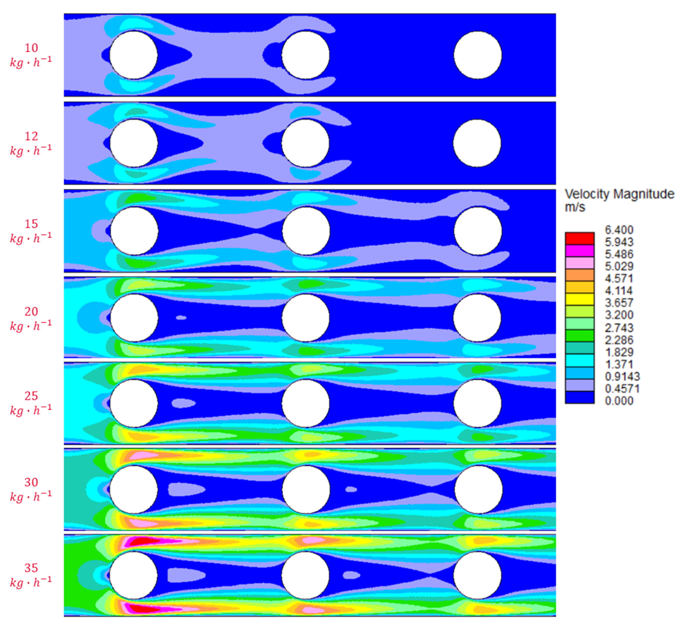
24 mm channel: 10; 12; 15; 20; 25; 30 and 35 kg∙h⁻¹, which corresponds to the vapor velocity range, in front of the first testing pipe, from 0.67 to 1.96 m∙s⁻¹.

(b)

20 mm channel: 10; 12; 15; 20; 25 and 30 kg∙h⁻¹, which corresponds to the vapor velocity range, in front of the first testing pipe, from 0.81 to 2.32 m∙s⁻¹.

On the cooling water side, its volumetric flow rate (${\dot{V}}_3$) was set, which had to be within the range of 7.5 ± 0.1 L∙min⁻¹. Throughout all the experiments, its average value was 7.51 ± 0.05 L∙min⁻¹. Thanks to this, the experiments were carried out under approximately equal conditions; the average value of the Reynolds number on the cooling water side, with all the experiments included, was 22,623 ± 3029 and the average value of the Nusselt number was 104.4 ± 6.6, without distinguishing the required temperature of the cooling water at the inlet into the exchanger. For all the required vapor mass flow rates, three temperature levels were tested of the cooling water at the inlet into the exchanger ($T_3$), in particular 30, 40 and 50 °C, with a permissible deviation of up to ±1.0 °C. The resulting average temperatures of the cooling water at the inlet into the exchanger were 30.5 ± 0.2 °C, 40.1 ± 0.2 °C and 50.0 ± 0.1 °C.

3. Results and Comparison

3.1. Results of the Experiments

The presented results were determined based on the mean value of the data set measured for each condition described in Section 2.3. The condensation heat transfer coefficient depends on the condensing power transferred in the heat exchanger. The graph in Figure 2 shows the development of the power transferred during condensation for the input cooling water temperatures of 30, 40 and 50 °C (blue, orange and red colour) and for the conditions with a regular channel (24 mm: full points and continuous curve) and with a reduced channel (20 mm: empty points and dashed curve). The graph clearly indicates that the channel width was relatively negligible, and that the deviations fell within statistical errors. The input cooling water temperature had a non-negligible effect. The lower the cooling water temperature, the higher the heat flow in the exchanger. By reducing the cooling water temperature by 20 °C, the output of the heat exchanger increased by approx. 25% on average. It is apparent from the graph that the output of the exchanger increased with the velocity of the vapor very slowly, which indicates that increasing the vapor flow rate and thus increasing the velocity of the vapor flow along the pipes had a negligible effect on the power transferred. Only when the vapor mass flow rate was reduced below 12 kg·h⁻¹ did the output of the exchanger start to decrease for lower cooling water temperatures, because almost all the vapor in the exchanger condensed and, therefore, the power transferred was a function of the vapor mass flow rate. It can be assumed, based on this trend, that the influence of the input cooling water temperature started to be negligible below a vapor flow rate of 10 kg·h⁻¹.

The power transfers in the exchanger are supplemented by the logarithmic temperature gradient values for each mode shown in Figure 3. The figure clearly shows that the logarithmic temperature gradient copies the development of the power transferred, and that the developments are almost constant in the vapor flow rate interval from 12 kg·h⁻¹ to 30 kg·h⁻¹. Below a water vapor flow rate of 12 kg·h⁻¹, and for the input cooling water temperature of 30 °C, a slight increase occurs due to a decrease in the output of the exchanger, and thus, less heating of the cooling water occurs. Above 30 kg·h⁻¹ of the water vapor, the logarithmic temperature gradient increases again. This is caused by an increase in the pressure inside the exchanger due to the mass flow rate being too high and thus the saturation vapor temperature increasing.

Based on the identification of the power transferred and the heat transfer coefficients, the condensation coefficient of heat transfer on the external side of the pipes can be derived from Equation (7). Its values are shown in Figure 4. For the particular geometry of the exchanger, it holds that with a higher vapor mass flow rate, and thus, its higher velocity, the condensation heat transfer coefficient increases. This is true up to a flow rate of 25 kg·h⁻¹, where the maximum is reached, and with a further increase in the vapor mass flow rate, it starts decreasing.

Considering this fact and taking into account the power transferred, it can be stated that the optimum water vapor flow rate for this exchanger geometry is 25 kg·h⁻¹. The graph shows that the highest values for each condition measured are reached in the mode with an input cooling water temperature of 30 °C. With the temperature increasing, the condensation heat transfer coefficient decreases. This trend applies to the presented interval of the vapor mass flow rate ranging from 12.5 kg·h⁻¹ to 35 kg·h⁻¹. Below 12.5 kg·h⁻¹ of vapor, with the input cooling water temperatures being 30 °C and 40 °C, the condensation heat transfer coefficient starts to decline rapidly; below this flow rate, it holds that with the cooling water temperature increasing, the condensation heat transfer coefficient increases. This is caused by the output of the exchanger decreasing, as shown in Figure 2. When comparing the wider and the narrower channels, one comes to the conclusion that the width of the channel plays a negligible role. Only with the vapor mass flow rate exceeding 25 kg·h⁻¹ does the condensation heat transfer coefficient reach higher values in the narrower channel than in the wider channel. The difference between heat transfer in the narrower channel and in the wider one is around 5%. Below a vapor flow rate of 25 kg·h⁻¹, the behaviour of the condensation heat transfer coefficients is very similar for both channel widths.

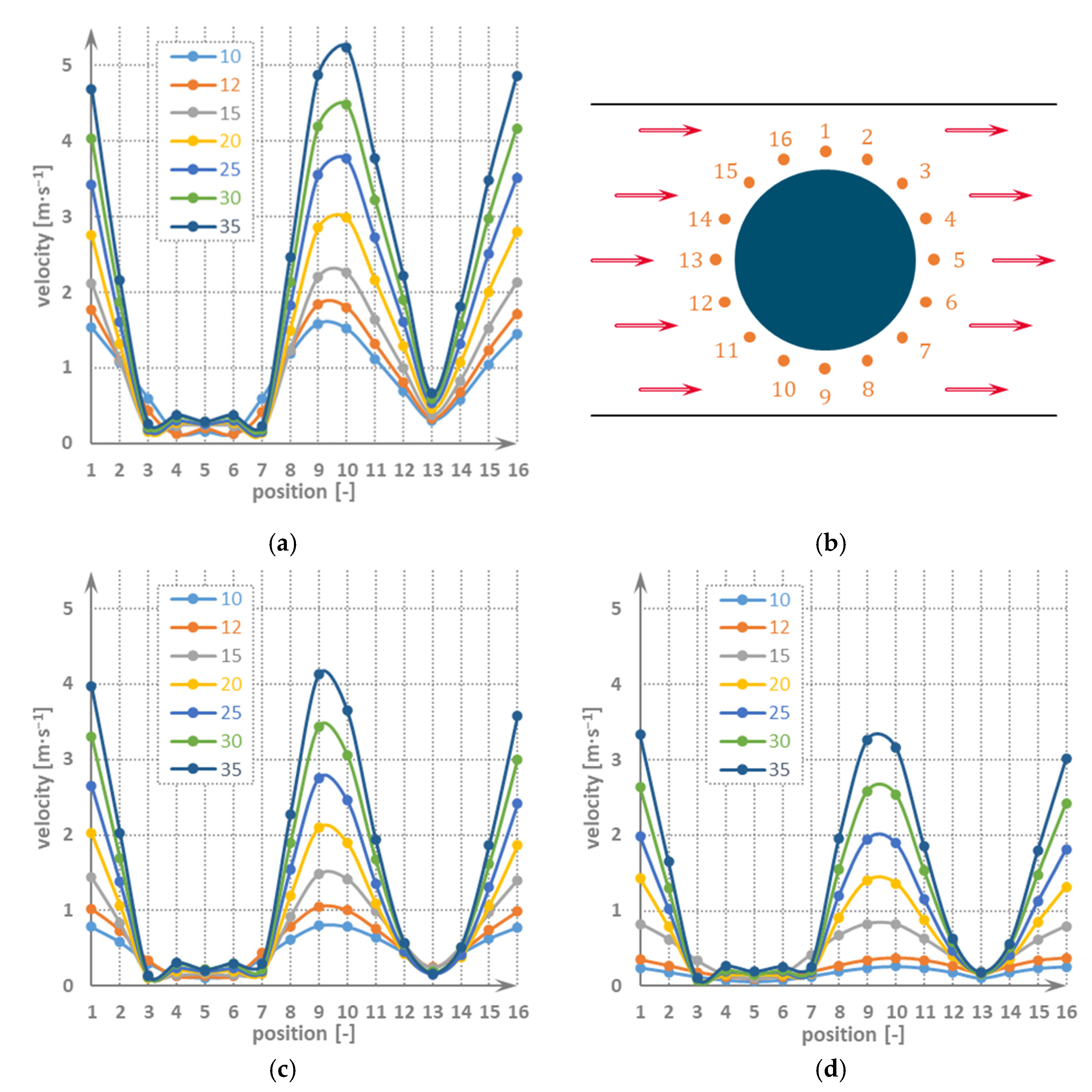
3.2. Steam Flow Identification by Computational Modeling

For a detailed identification of 3D velocity fields and pressure fields in the studied exchanger, numerical modelling was used based on the finite volume method (FEM). The geometry of the channel with a width of 24.0 mm with three vertical pipes, shown in Figure 1, was accurately transformed into a structured computational network formed by hexagonal control volumes. Smaller control volumes are used near the surface of the vertical pipes. Larger control volumes are used in the space between the pipes. This enables an accurate and rapid simulation to be generated of the flow situations around the pipes.

The Simcenter STAR-CCM+ commercial SW package was used for this purpose. Equations respecting the laws of conservation of matter, energy and momentum form the basis of the computational algorithms used. The calculation was performed for a compressible turbulent water vapor flow. The K-omega SST turbulence model was used as a suitable model to obtain a correct description of processes near solid surfaces. The static enthalpy thermal model was used in the computational solution of the energy transformation balance.

The INLET boundary condition is assigned to the surface through which the vapor enters the computational area. On this surface, an input vapor flow velocity was set ensuring the required vapor mass flow at a given temperature and pressure. The PRESSURE boundary condition was assigned to the wall of the model through which the vapor leaves the area. On this wall, a value of static pressure was determined from the experimental measurements conducted. The vapor velocity field in the studied channel was significantly affected by vapor condensation on the surface of the vertical pipes being cooled down. A detailed inclusion of the condensation process in the computational model is a task that is very difficult in terms of the solver setup and places enormous demands on the computing time. The main problem of such a solution is the vapor phase change and the subsequent flow of liquid with a free surface. In this study, a simplified approach without the phase change was applied in order to include the influence of condensation on the vapor velocity field. In the first step, the amount of condensing vapor was analytically calculated. In the second step, the computational model was set so that the same amount of vapor would be virtually “sucked out” through the walls of the heat exchanger pipes in the model. With such simplification, it is not necessary to deal with the water phase change and, at the same time, the effect of the condensation process on the vapor velocity field is taken into account.

The computational model was used for a parametric study including seven vapor mass flow rate conditions corresponding to the conducted experiments. The results of the numerical calculations are shown as velocity fields in Figure 5. All the cases shown include a non-narrowed channel with a width of 24 mm and a cooling water temperature at the inlet into the first pipe of 30 °C, on average. The experimental data in the analytical model were used to determine the amount of vapor condensing on each pipe.

Figure 6 shows the vapor flow velocities that were evaluated in detail in the distance of one tenth of the pipe diameter (i.e., 1.4 mm from the pipe wall). The development of the velocities clearly shows that the highest vapor flow velocity occurs on the first pipe, while on the other pipes, the velocity decreases. This is caused by continuous vapor condensation. The figure shows that the flow velocity is not the same along the perimeter. There are areas with a high flow velocity (sides of the pipe—points 16, 1, 10 and 9) and areas with almost zero flow (the thrust side and the rear side of the pipe—points 3 to 7). This means that the condensation flow along the pipe perimeter is not constant, and there are significant differences. Additionally, the real size of the heat exchange surface, where heat transfer occurs, will be smaller than the total area of the pipes. This phenomenon is then probably the reason why there was an optimal mass flow rate for this exchanger geometry, as mentioned in the comment on Figure 4. With a mass flow rate of 25 kg·h⁻¹, the ratio between the flow velocity and the real size of the heat exchanging surface was optimal.

Generally, the velocity of saturated vapor flowing in a channel with the mass flow rate $\dot{M_i} \left[\mathrm{kg}·{\mathrm{s}}^{-1}\right]$ on the surface $S_i \left[{\mathrm{m}}^2\right]$ can be determined as

$$w_i=\frac{{\dot{M}}_i}{ S_i·{\rho }_v} \left[\mathrm{m}·{\mathrm{s}}^{-1}\right].$$

(13)

When comparing the vapor velocity in front of the pipe from the analytical model and the average velocity determined by the velocities at the points (1–16) around the pipe based on Figure 6, the relative deviation (error) between these velocities ranges from −17% to 22%. The situation is similar when comparing the median value of the velocities at the points (1–16) and the analytically calculated value, where the deviations range from −49% to 24%. This means that there is no direct correlation between the average velocity around the pipe and the velocity in front of the pipe.

Figure 6 clearly shows the maximum velocities at points 16, 1, 10 and 9 for all three pipes. At the same time, the analytical model can be used to calculate the maximum velocity at the narrowest point around the pipe. What is unknown, however, is the amount of vapor that condenses on the front part of the pipe in front of the narrowest point. This is why a parametric study was conducted aiming to determine the real amount of vapor flowing through the narrowest point, as follows:

$${\dot{M}}_i={\dot{M}}_p-x·{\dot{M}}_k \left[\mathrm{kg}·{\mathrm{s}}^{-1}\right],$$

(14)

where ${\dot{M}}_p$ is the vapor mass flow rate in front of the pipe, ${\dot{M}}_k$ is the condensed vapor mass flow rate on the given pipe and $x$ takes into account the amount of condensed vapor in front of the narrowest point. Figure 7 shows the relative error of the maximum velocity determined from the CFD model (the average value of the points 16, 1, 10 and 9) and the maximum velocity based on Equations (13) and (14), where the error was determined as follows:

$$relative error=\frac{w_{CFD\left(16,1,10,9\right)}-w_{max\left(x·{\dot{M}}_k\right)}}{w_{CFD\left(16,1,10,9\right)}}·100 [\%].$$

(15)

Figure 7 clearly shows that the largest deviations occur at the lowest velocities for $x=0.00$, i.e., no vapor condenses in front of the narrowest point, and for $x=1.00$, i.e., all the vapor condenses in front of the narrowest point. The optimal value appears to be $x=0.33$, i.e., one third of the vapor condenses in front of the narrowest point and the average error calculated from the absolute values of the relative error is 7.4%. For $x=0.25$, the average error calculated from the absolute values reaches 9.6%, and for $x=0.50$, it is 9.1%.

3.3. Comparison with Other Studies

The following subchapter offers a comparison of the results with other studies. As was mentioned in the introduction, there are not many relevant studies on pure water vapor condensation on the external side of a vertical pipe. For comparison, relevant analytical relationships by four authors were selected as models S1, S2, S3 and S4.

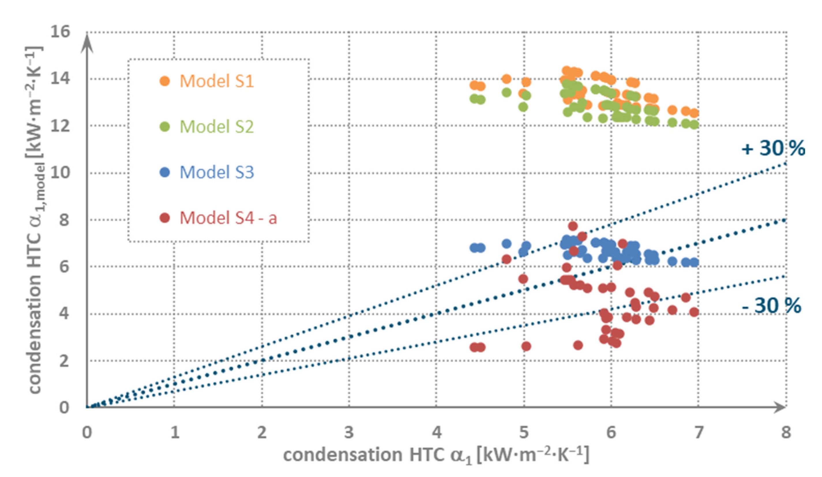
3.3.1. Model S1

In his paper from 1916 [3], Nusselt published a formula for calculating the Nusselt number. He derived the gravitational theory for laminar film. His formula is as follows:

$$N{u}_{1,S1}=0.729·{\left[\frac{g·r·d_1^3·\left({\rho }_f-{\rho }_v\right)}{{\nu }_f·{\lambda }_f\left(T_1-T_{S1}\right)}\right]}^{1/4} [-],$$

(16)

where $d \left[\mathrm{m}\right]$ is the pipe diameter and $g=9.81 \left[\mathrm{m}·{\mathrm{s}}^{-2}\right]$ is gravitational acceleration. The mean thermal conductivity of the condensate is determined in relation to the mean temperature of the condensate given by the condensation temperature, $t_1 \left[°\mathrm{C}\right]$, and by the temperature of the pipe wall, $t_{S1} \left[°\mathrm{C}\right]$, which is determined by Equation (18),

$${\lambda }_f=f\left[p_{sat}\left(t_1\right);\frac{t_1+t_{S1}}{2}\right] \left[\mathrm{W}·{\mathrm{m}}^{-1}·{\mathrm{K}}^{-1}\right],$$

(17)

with the temperature of the pipe wall, $t_{S1} \left[°\mathrm{C}\right]$, being based on the heat flow and resistance to heat conduction as:

$$T_{S1}=T_1-\frac{{\dot{Q}}_S}{\pi ·d_1·L·n·{\alpha }_1} \left[\mathrm{K}\right],$$

(18)

the density of the saturated condensate being determined as

$${\rho }_f=f\left(t_1;x=0\right) \left[\mathrm{kg}·{\mathrm{m}}^{-3}\right],$$

(19)

the density of the saturated vapor being determined as

$${\rho }_v=f\left(t_1;x=1\right) \left[\mathrm{kg}·{\mathrm{m}}^{-3}\right],$$

(20)

the condensation (vaporisation) heat of the condensate being determined as

$$r=i\left(t_1;x=1\right)-i\left(t_1;x=0\right) \left[\mathrm{J}·{\mathrm{kg}}^{-1}\right],$$

(21)

and the kinematic viscosity of the condensate being determined as a ratio of dynamic viscosity to the density determined in relation to the mean condensate temperature

$${\nu }_f=\frac{{\mu }_f}{{\rho }_f}=f\left[p_{sat}\left(t_1\right);\frac{t_1+t_{S1}}{2}\right] \left[{\mathrm{m}}^2·{\mathrm{s}}^{-1} \right].$$

(22)

The coefficient of heat transfer on the external side of the pipe can then be calculated from the Nusselt number as

$${\alpha }_{1,S1}=\frac{Nu·{\lambda }_f}{d_1} \left[\mathrm{W}·{\mathrm{m}}^{-2}·{\mathrm{K}}^{-1}\right]$$

(23)

3.3.2. Model S2

Nusselt was followed up by Rohsenow‘s publication [15], where the original Nusselt’s formula was slightly modified, as follows:

$$N{u}_{1,S2}=0.707·{\left[\frac{g·r·d_1^3·{\rho }_f}{{\nu }_f·{\lambda }_f·\left(T_1-T_{S1}\right)}\right]}^{\frac{1}{4}} [-]$$

(24)

and the coefficient of heat transfer on the external wall can be expressed from the Nusselt number using Equation (23).

3.3.3. Model S3

In his paper [14], Incropera published a formula for the direct calculation of the heat transfer coefficient, as follows:

$${\alpha }_{1,S3}=0.943·{\left[\frac{{\lambda }_f^3·\left({\rho }_{1f}-{\rho }_{1v}\right)·r·g}{{\nu }_f·\mathsf{\Delta }t·h}\right]}^{0,25} \left[\mathrm{W}·{\mathrm{m}}^{-2}·{\mathrm{K}}^{-1}\right],$$

(25)

where the characteristic dimension $h \left[m\right]$ corresponds to the height of the pipe (channel).

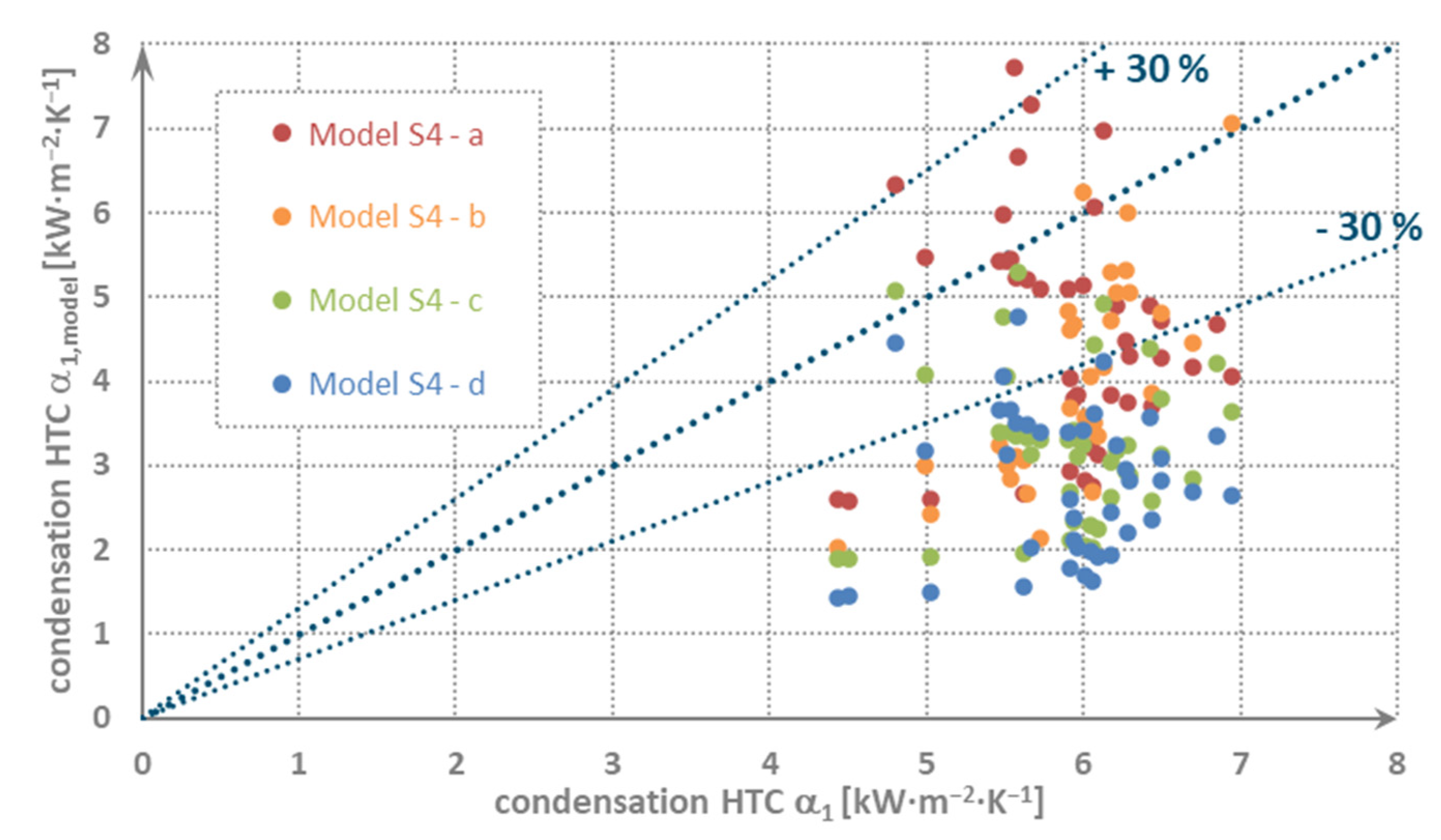
3.3.4. Model S4

The last study being compared is that by Chang [11], which analysed the steady mixed convection of a condensate film running along an isometric vertical pipe in dry saturated vapor with forced flow. In this publication, Chang proposed a formula for the Nusselt number, which uses the Reynolds, Prandtl, Grashof and Jacob numbers as follows:

$$N{u}_{1,S4}=\frac{4^{\frac{1}{4}}·{\xi }^{\frac{1}{2}}·K·{\left(1+\frac{P{r}_f}{4·K^4·{\xi }^2·Ja}\right)}^{\frac{1}{4}}}{{\left(\frac{Gr}{4}\right)}^{-\frac{1}{4}}} [-],$$

(26)

where

$$K=0.45·{\left(1.2+\frac{P{r}_f}{Ja}\right)}^{\frac{1}{3}} [-],$$

(27)

$$\xi =\frac{R{e}_{v,max}}{G{r}^{1/2}} [-],$$

(28)

$$Gr=\frac{g{d}_1^3}{{\nu }_v{}^2} [-],$$

(29)

$$Ja=\frac{c_{p,f}·\left(T_1-T_{S1}\right)}{r} [-],$$

(30)

$$R{e}_{v,max}=\frac{w_{1\max }·d_1}{{\nu }_v} [-]..$$

(31)

The Reynolds number is calculated with the maximum velocity, which is reached in the heat exchanger in question between the heat exchanger and pipe walls. The velocity is calculated as:

$$w_{1max}=\frac{S_T·w_1}{S_T-d_1} \left[\mathrm{m}·{\mathrm{s}}^{-1}\right]$$

(32)

$$S_T=\frac{d_1}{2}+\frac{b}{2} \left[\mathrm{m}\right]$$

(33)

where $b \left[\mathrm{m}\right]$ is the width of the free channel.

3.3.5. Comparing the Models with the Experimental Results

Figure 8 shows a comparison of the models with the condensation heat transfer coefficient determined in the experiments. The points of models S1 to S4 were derived based on the relevant states measured. The developments do not take into account the temperature of the cooling water entering the first pipe of the exchanger or the width of the channel, since their effects are negligible. The graph also shows the bands of error, specifically, ±30%.

Figure 8 clearly shows fairly good agreement with model S3, which is the only one that does not take into account the diameter of the pipe on which the water vapor condenses but does factor in the height of the heat exchanging surface.

Table 1. Statistical evaluation of each variant.

Model	Average Error [%]	Standard Deviation [%p]
S1	−131.3	±28.5
S2	−121.9	±27.3
S3	−14.7	±14.4
S4—a	23.4	±19.3
S4—b	34.1	±19.5
S4—c	45.3	±13.2
S4—d	53.6	±13.1

presents the basic statistical data from the comparison of the models. In particular, the average error, i.e., in the case of the best agreement with model S3, the experimental values are 14.7% lower and the average value band (standard deviation of error) is ±14.4%_p (of a percentage point).

Figure 8 shows variant ″a″ for model S4 and Table 1, and offers a comparison of the other three variants. Although model S4 takes into account the vapor flow velocity, several variants were tested. In particular,

(a)

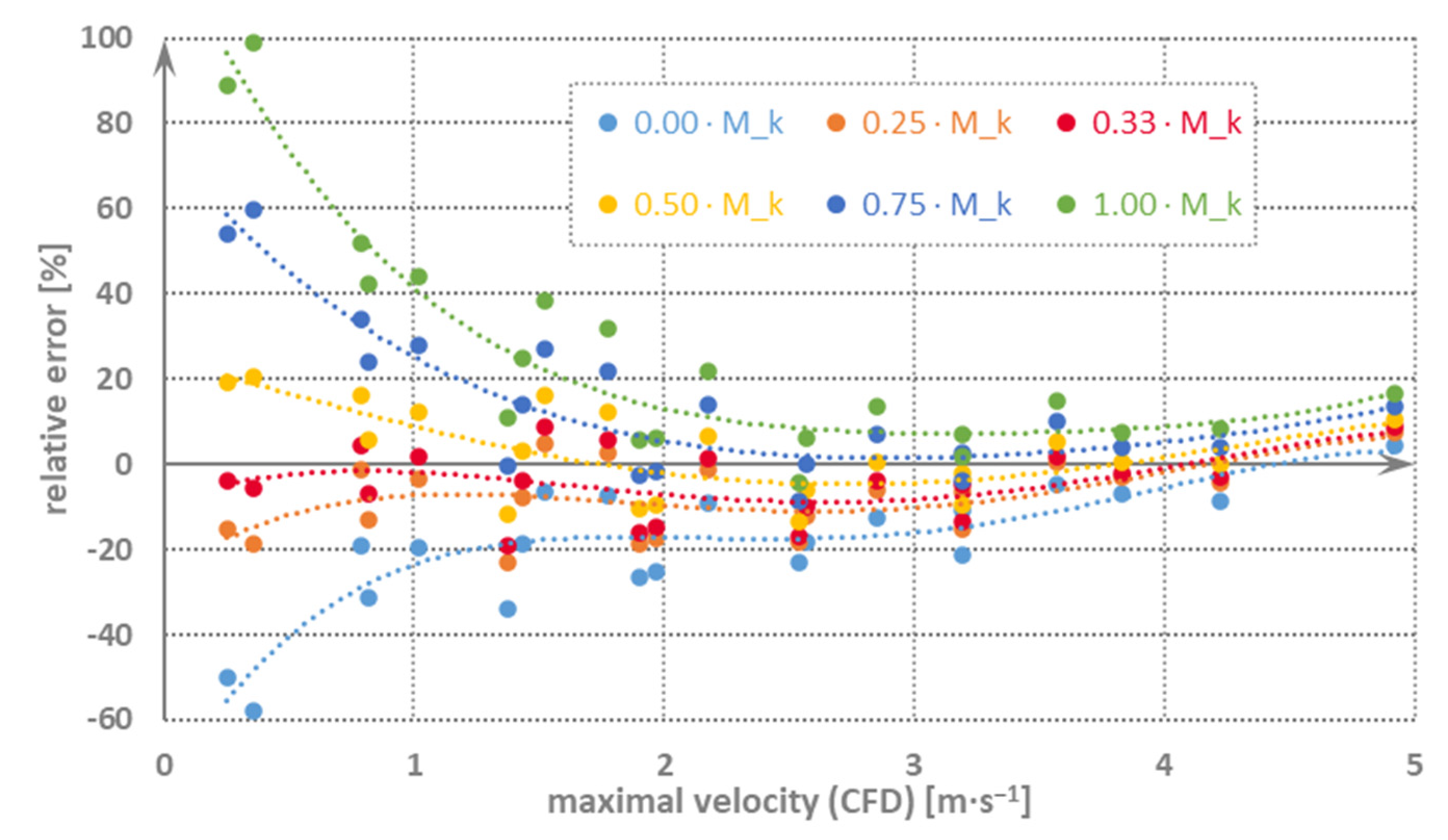
The basic variant when the authors calculate the Reynolds number from the maximum velocity; see Equation (31). The maximum velocity is determined on the basis of the pipe bundle geometry (spacing of the pipes/row), where, in our case, another adjacent pipe is the channel wall. The velocity considered in this variant is that in front of the first pipe.

(b)

Another variant is the mean value of the vapor velocity in front of all the three pipes, i.e., the average value of the vapor velocity in front of the first, second and third pipes. This value is then adjusted as in the previous variant, i.e., it is substituted into Equation (32) and then into Equation (31).

(c)

Based on Equations (13) and (14), the maximum velocity at the narrowest point around the first pipe is determined. The amount of condensed vapor in front of the narrow section is $x=0.33$. This velocity is directly substituted into the calculation of the maximum Reynolds number in Equation (31).

(d)

As in the previous variant, the maximum vapor velocity is calculated at the first, second and third pipes, and these values are used to calculate the average maximum velocity. This velocity is directly substituted into the calculation of the maximum Reynolds number in Equation (31).

The different variants of model S4 are compared in Figure 9, which clearly shows the systematic shifting of the variants in relation to each other. Based on Table 1, the most suitable way of calculating model S4 is with variant “a”, which is, nevertheless, worse than model S3.

4. Conclusions

The paper was focused on the condensation of water vapor on vertical pipes. To identify the condensation heat transfer coefficient, a series of experiments was performed in a heat exchanger with condensation on the external side of the vertical pipes. The tubes were placed in a narrow channel simulating a normal tube bundle with a free gap at the narrowest width of 3.0 or 5.0 mm between the tube and the channel wall. The steam flowed in a crosswise direction around the vertical pipe. The influence of the input parameters on the resulting heat transfer can be summarised as follows, based on the experimental results:

(a)

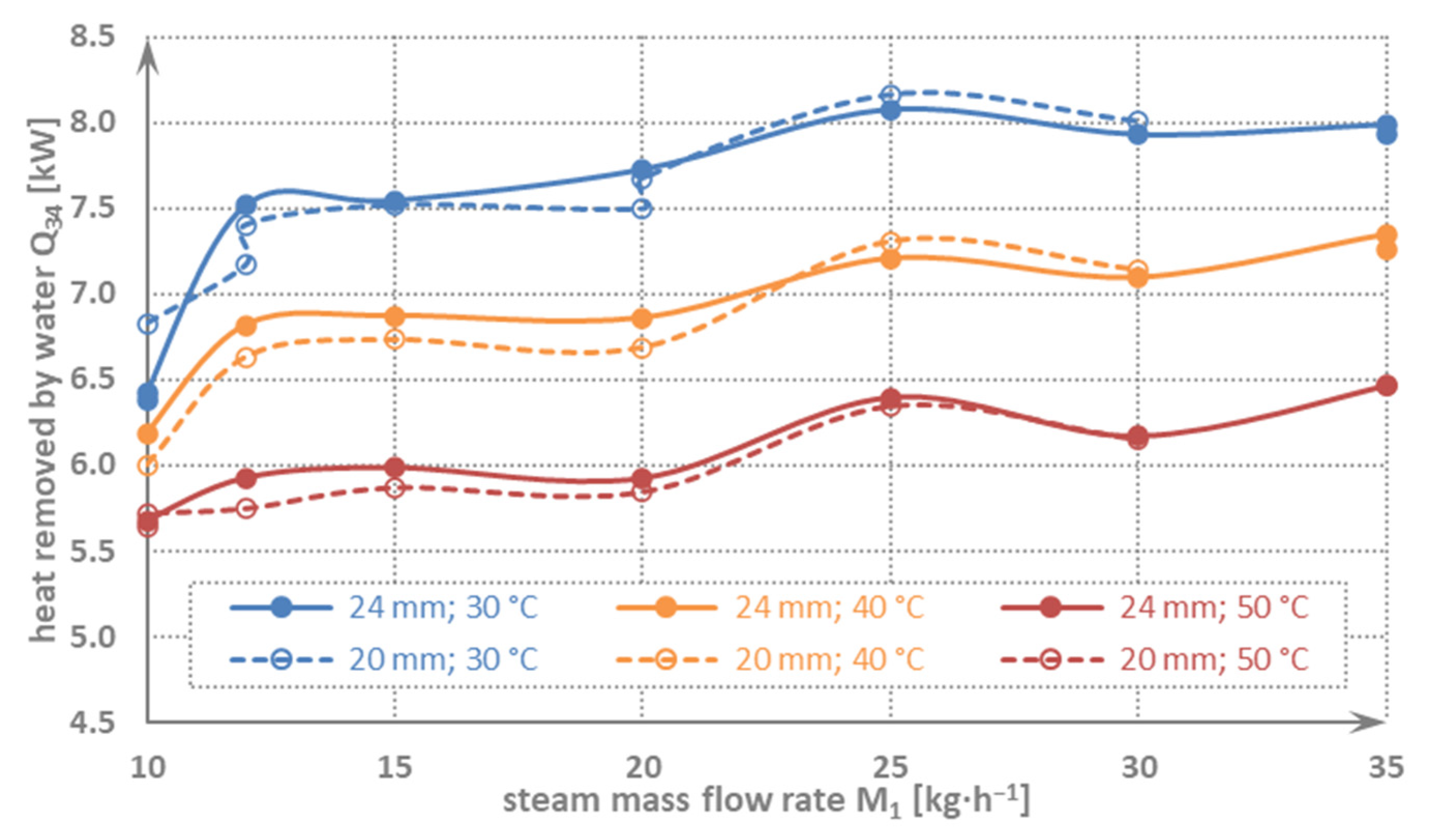
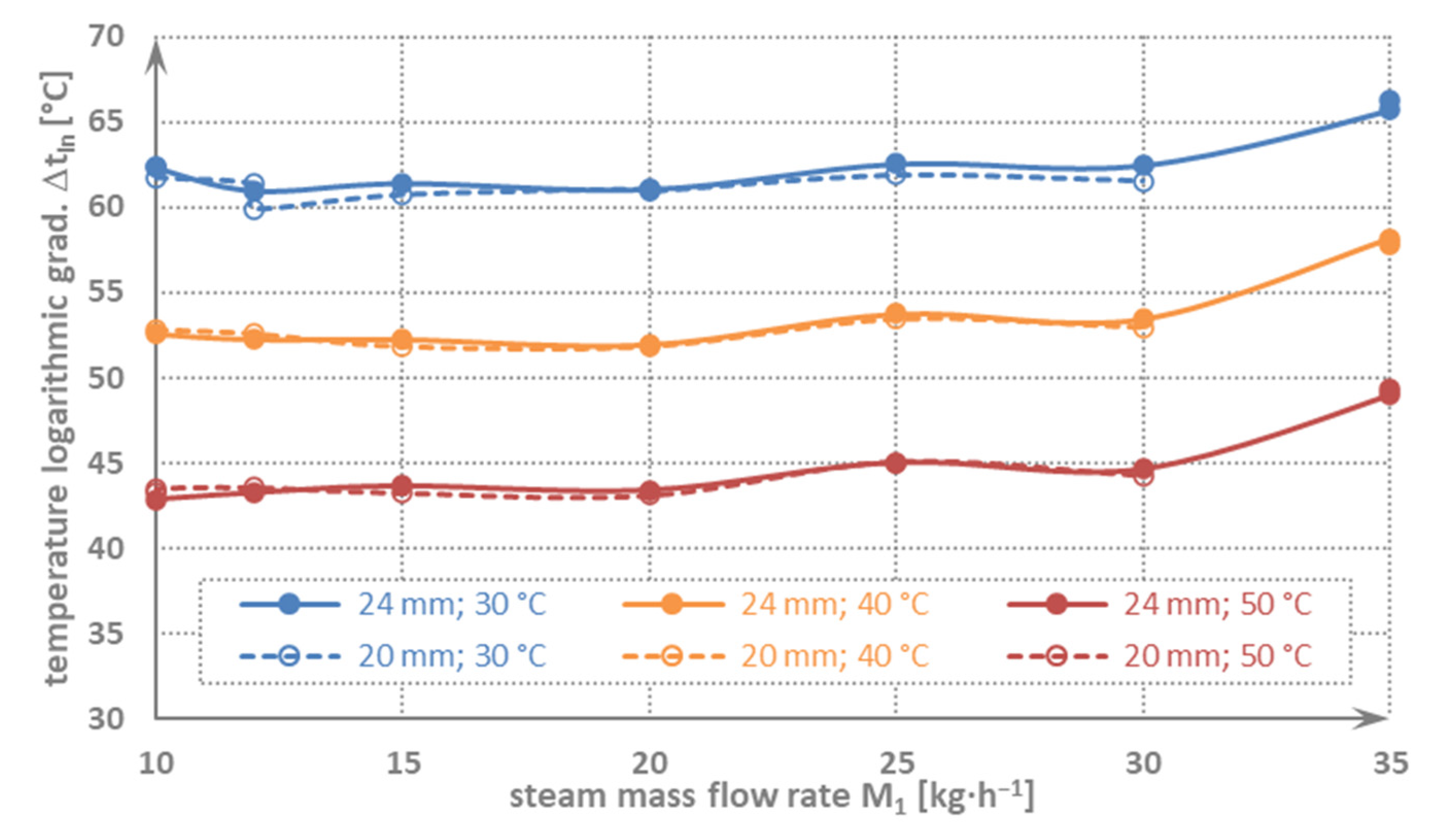
The width of the channel is negligible, and deviations fall within the statistical error margins.

(b)

The heat flow in the exchanger increases with a decreasing input temperature of the cooling water. By decreasing the temperature of the cooling water by 20 °C, the output of the exchanger increases by approx. 25%, on average.

(c)

At the moment when not all the vapor condenses in the exchanger, the influence of the vapor velocity at the inlet into the exchanger decreases.

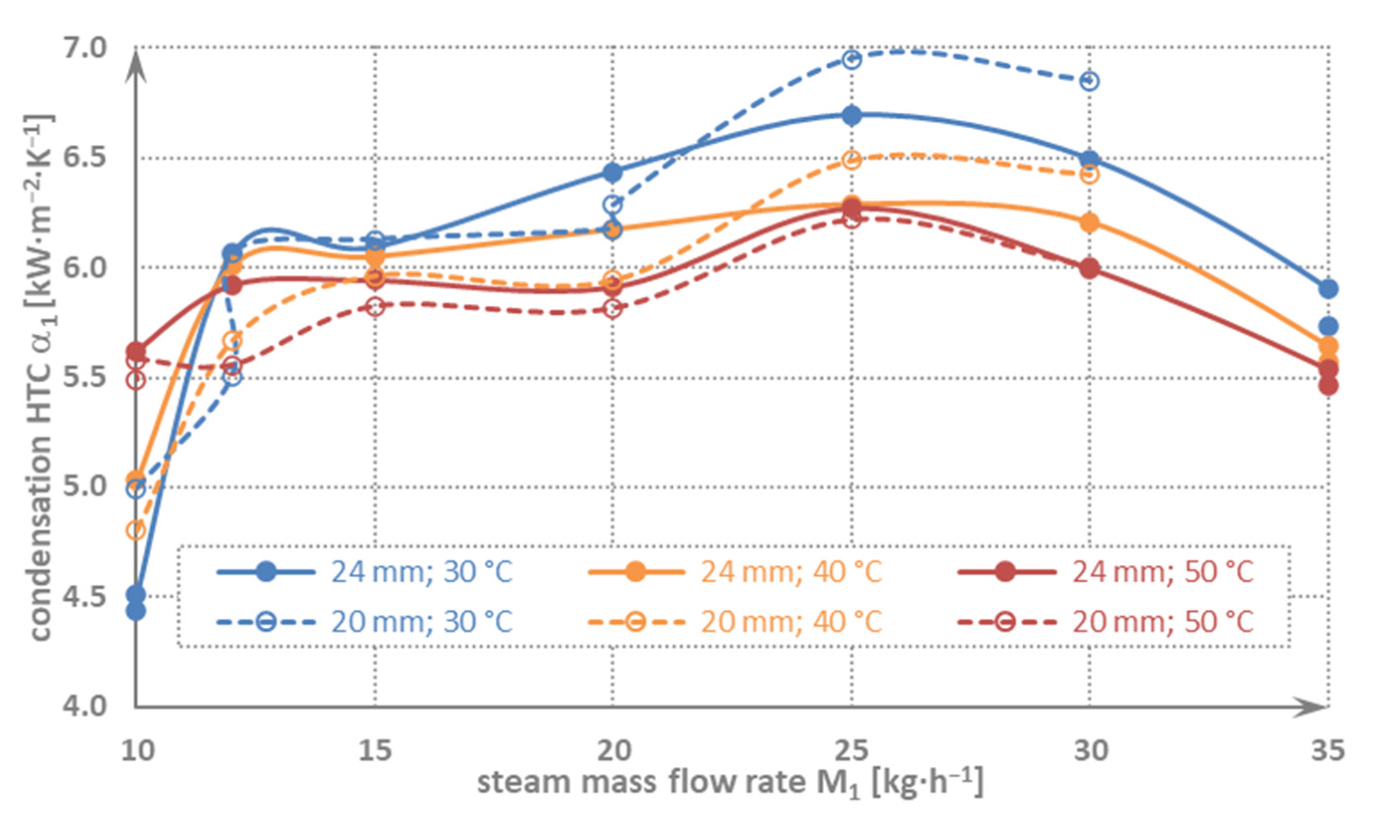
(d)

It holds for the particular exchanger geometry that with a higher vapor mass flow rate, and thus, a higher velocity, the condensation heat transfer coefficient also increases up to a flow rate of 25 kg·h⁻¹, where the maximum is reached; with a further increase in the flow rate, it starts decreasing.

The CFD simulation showed that the vapor flow velocity is not the same along the pipe perimeter, but there are areas with a high flow velocity and areas with almost zero flow (the thrust side and the rear side of the pipe). This is why the condensation flow is not constant along the pipe perimeter, and the effect of optimal operational vapor flow rate occurs here, which, for the particular geometry, corresponds to 25 kg·h⁻¹, at which the best ratio is achieved between the flow velocity and the real size of the heat exchanging surface, which is smaller than the theoretical area size given by the pipe shell.

In the final stage of the research, a comparison was made of the obtained results and those presented in studies by other authors. The studies do not directly deal with the cross flow of steam in the vicinity of a vertical pipe, but rather, with the condensation of steam on a vertical pipe with an ambiguous flow direction, i.e., in a larger space. The aim was to quantify the difference between the analytical relationships for vapor condensation on a vertical pipe and the results of an experiment with condensation of vapor on vertical pipes in a narrow channel. The best agreement between the analytical part and the experiment occurred for the formula by Incropera, who presents a direct calculation of the coefficient of stationary vapor heat transfer on the external side of a vertical pipe where the characteristic dimension is the pipe height. The average difference between the condensation heat transfer coefficient value obtained experimentally and the one determined analytically is −14.4% in favour of the analytical model. In the case of the Nusselt and Rohsenow model, which corrected Nusselt’s model, the results of the analytical models were at a similar level, but roughly twice higher than the results from the experiments. The last comparative study was by Chang. In this study, the velocity of the steam around the pipes was taken into account, but the results of the analytical model were one-third to one-half lower compared to the experimental results according to the applied steam flowing velocity. Although there was a good agreement for some conditions, it was not possible to draw a universal conclusion from them, nor to correct the semi-empirical relationships. After analysing the individual models, Incroper’s model can be recommended for this type of heat exchanger.

References

- Bhuyan, D.; Giri, A.; Lingfa, P. Entropy Analysis of Mixed Convective Condensation by Evaluating Fan Velocity With a New Approach. J. Therm. Sci. Eng. Appl. 2018, 10, 051003. [Google Scholar] [CrossRef]
- Miller, C.; Neogi, P. Interfacial Phenomena: Equilibrium and Dynamic Effects, 2nd ed.; CRC Press/Taylor & Francis: Boca Raton, FL, USA, 2008; ISBN 9781420044423. [Google Scholar]
- Nusselt, W. Die Oberflächenkondensation des Wasserdampfes. Z. Ver. Dtsch. Ing. 1916, 60, 541–546. [Google Scholar]
- Sparrow, E.; Gregg, J. A Boundary-Layer Treatment of Laminar-Film Condensation. J. Heat Transf. 1959, 81, 13–18. [Google Scholar] [CrossRef]
- Aktershev, S.; Alekseenko, S. The Stability of a Condensate Film Moving under the Effect of Gravity and Turbulent Flow of Vapor. High Temp. 2003, 41, 79–87. [Google Scholar] [CrossRef]
- Aktershev, S.; Alekseenko, S. Nonlinear waves in a falling film with phase transition. J. Phys. Conf. Ser. 2017, 899, 032001. [Google Scholar] [CrossRef] [Green Version]
- Jacobs, H. An integral treatment of combined body force and forced convection in laminar film condensation. Int. J. Heat Mass Transf. 1966, 9, 637–648. [Google Scholar] [CrossRef]
- Testu, F.; Haruo, U. Laminar filmwise condensation on a vertical surface. Int. J. Heat Mass Transf. 1972, 15, 217–233. [Google Scholar] [CrossRef]
- Winkler, C.M.; Chen, T.S.; Mi, W.J. Film condensation of saturated and superheated vapors along isothermal vertical surfaces in mixed convection. Numer. Heat Transf. Part A Appl. 1999, 36, 375–393. [Google Scholar]
- Zhao, Z.; Li, Y.; Wang, L.; Zhu, K.; Xie, F. Experimental study on film condensation of superheated vapour on a horizontal tube. Exp. Therm. Fluid Sci. 2015, 61, 153–162. [Google Scholar] [CrossRef]
- Chang, T. Mixed-convection film condensation along outside surface of vertical tube in saturated vapor with forced flow. Appl. Therm. Eng. 2008, 28, 547–555. [Google Scholar] [CrossRef]
- Tong, P.; Fan, G.; Sun, Z.; Ding, M.; Su, J. An experimental investigation of pure steam and steam–air mixtures condensation outside a vertical pin-fin tube. Exp. Therm. Fluid Sci. 2015, 69, 141–148. [Google Scholar] [CrossRef]
- Toman, F.; Kracík, P.; Pospíšil, J.; Špiláček, M. Comparison of Different Concepts of Condensation Heat Exchangers With Vertically Oriented Pipes for Effective Heat and Water Regeneration. Chem. Eng. Trans. 2019, 76, 379–384. [Google Scholar]
- Incropera, F. Fundamentals of Heat and Mass Transfer, 6th ed.; John Wiley & Sons: New York, NY, USA, 2007; ISBN 9780471457282. [Google Scholar]
- Rohsenow, W. Heat transfer and temperature distribution in laminar film condensation. Trans. Am. Soc. Mech. 1956, 78, 1645–1648. [Google Scholar] [CrossRef]