A Short-Term Photovoltaic Power Forecasting Method Combining a Deep Learning Model with Trend Feature Extraction and Feature Selection

Abstract

High precision short-term photovoltaic (PV) power prediction can reduce the damage associated with large-scale photovoltaic grid-connection to the power system. In this paper, a combination deep learning forecasting method based on variational mode decomposition (VMD), a fast correlation-based filter (FCBF) and bidirectional long short-term memory (BiLSTM) network is developed to minimize PV power forecasting error. In this model, VMD is used to extract the trend feature of PV power, then FCBF is adopted to select the optimal input-set to reduce the forecasting error caused by the redundant feature. Finally, the input-set is put into the BiLSTM network for training and testing. The performance of this model is tested by a case study using the public data-set provided by a PV station in Australia. Comparisons with common short-term PV power forecasting models are also presented. The results show that under the processing of trend feature extraction and feature selection, the proposed methodology provides a more stable and accurate forecasting effect than other forecasting models.

1. Introduction

World energy demand has increased steadily over the years. Today’s principal resources are oil and coal, but with finite supplies of fossil fuels and strong evidence of their negative environmental impact [1]. In addition to being non-renewable, fossil fuels also cause serious environmental pollution, which further leads to greenhouse gas emission, acid rain, ozone depletion and fossil fuel combustion [2]. Therefore, there is an urgent need to seek alternate sources of energy that are cleaner and more sustainable. Solar energy is a clean and renewable energy source. With the growing global demand for clean energy, photovoltaic (PV) power will play an important role. In past decades, PV power has attracted more and more attention [3,4]. PV power brings notable environmental benefits and economic results. However, PV power is indeterminate and intermittent, because the output power of a PV system depends on many random factors including global horizontal radiation, temperature, wind, and system components with their own non-linear factors, among others [5]. As a result, large scale integration of PV into the power grid brings many new risks to the operation of the existing power grid system. Increasing the precision of PV power prediction is effective in addressing these challenges.

There are various methods to predict the output of PV power. According to different prediction processes, short-term PV prediction is divided into direct-prediction and indirect-prediction [6]. Ref. [7] describes the use of Feature Attention Deep Forecasting (FADF) in a deep neural network to generate global horizontal irradiance forecasting. However, this kind of FADF based on a neural network is very sensitive to the disturbance of training data, and may reduce the robustness of FADF. Therefore, indirect-prediction is adopted in this paper. After long-term research at home and abroad, many short-term forecasting methods and algorithms have been used to predict PV power in a short time indirectly. Short-term PV power forecasting methods are divided into three types: (1) a conventional statistical model [8]; (2) an artificial intelligence model [9,10], and (3) a combination forecasting model. Much research has noted that no individual forecasting model is the best for all types of load forecasting. Therefore, it is necessary to combine different models to reduce the risk of making worse prediction.

Conventional statistical models include a time series model [11], a regression analysis model [12], grey theory [13] and fuzzy theory [14]. They mainly take historical data into account to forecast future data. These models predict PV power in future days by mining the relevance between input variables and output variables through historical data. However, these statistical models assume that the time series data are linear correlated, which does not reduce the error caused by the intermittence of PV, and lead to poor prediction results.

Artificial intelligence is developing rapidly, especially in deep learning. As deep learning can capture the variation rule of PV power and the complicated relationship between PV power and meteorological factors, numerous artificial intelligence models are applied to PV power forecasting such as artificial neural networks (ANNs) [15] and long short-term memory (LSTM) [16], among others. These models can improve the problem of poor accuracy of conventional statistical models. Currently, most deep learning models are used to predict short-term PV power combined with feature selection and data processing algorithms. In Ref. [17], the authors used a technique combining a decomposition model with a deep learning network to predict 1-h PV power output. In [18] a restricted Boltzmann machine (RBM) deep neural network was used with multi-layer perceptron (MLP) and predator-prey brainstorm optimization of evolutionary computation to obtain better predicted values. Ref. [19] proposes a new forecasting method based on a recurrent neural network (RNN) to predict PV power generation. Ref. [20] proposes a hybrid approach based on a convolutional neural network (CNN) and LSTM for PV power forecasting.

PV power and solar spectral irradiance are closely related, and solar spectral irradiance is usually affected by other meteorological factors, so the characteristics of PV power are different under different weather conditions. This means that the accuracy of PV power prediction depends not only on the historical load data, but also on weather factors [21,22]. Ref. [23] proposes a method based on a feature matrix and LSTM. A short-term PV power prediction model combined generative adversarial networks with convolutional neural networks-based weather classification is proposed in [24]. In Ref. [25], it is mentioned that the data quality of neural network training samples and the selection of numerical weather prediction (NWP) factors also have a certain impact on short-term PV power prediction. In addition, models used in Refs. [26,27,28] have a similar prediction pattern to the proposed model, using meteorological data and historical PV power for short-term PV prediction. The mean absolute percentage error (MAPE) of these models 1-day ahead of PV prediction is about 20%, while the MAPE in this paper can reach 13.84% and 5.21%.

In addition to improving the performance of the forecasting model, measures to reduce the error of short-term load forecasting may include trend feature extraction and feature selection.

Trend feature can reflect the unique power characteristics of different stations, and it is worth noting that the characteristics of PV power are mainly affected by local climate, longitude and latitude, and terrain. It not only describes the relationship between the growth and change of PV power with time, but also illustrates the short-term effects and interactions among PV power. However, many researchers only use historical load data and meteorological information to predict the PV power and cannot determine the dynamic changing process of PV, which is not conducive to improvement of short-term PV power forecasting. In Ref. [29], an improved CEEDMAN algorithm is used to extract a meaningful sub-mode in the PV power to reduce prediction error caused by noise. In addition, the input dimension of the prediction model also affects prediction accuracy. Before prediction, it is necessary to find the main factors affecting the change of PV power and remove redundant variables. In Ref. [30], the authors use a random-forest approach to calculate and rank the affecting factors and select the optimal feature-set to improve forecasting accuracy.

Based on the above analysis, a novel short-term PV power forecasting method combined BiLSTM with trend feature extraction and feature selection is proposed in this paper. According to the mathematical principle of VMD, the original PV power is decomposed into multiple intrinsic mode functions (IMFs), and then the trend feature of PV power is extracted from a series of IMFs. To further reduce the prediction error caused by high feature dimensions, the FCBF algorithm was not applied to PV prediction to extract the optimal feature-set from meteorological data, historical PV power and trend feature. In the short-term the PV power forecasting model uses the BiLSTM model and takes the input set filtered by FCBF as the input-variables to predict the PV power of a PV power station from Alice Spring in Australia. The model can fully determine the change of PV power and increase the efficiency of the prediction model. Finally, example analysis shows that compared with other prediction methods, the model has advantages in prediction effect and can significantly increase the accuracy of short-term PV power forecasting.

The main contributions of this study are as follows:

• An effective trend feature extraction method is developed to extract the trend feature of PV power;
• Trend feature, meteorological data and historical PV power data are used to select the optimal input feature by a FCBF algorithm;
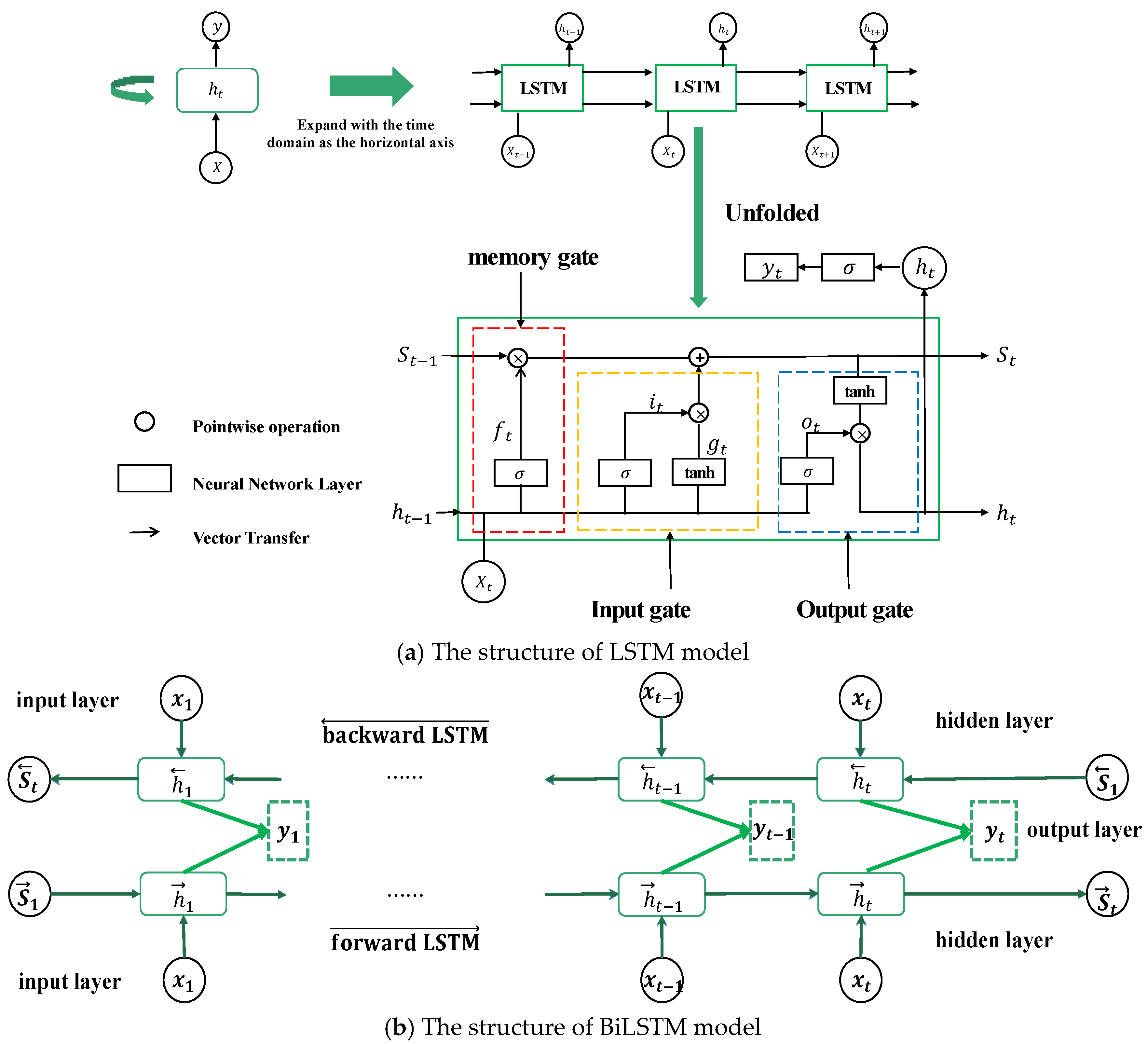
• A BiLSTM model is adopted to predict PV power with high accuracy;
• The proposed model is compared with different PV forecasting models.

The rest of this paper is organized as follows. Section 2 presents the framework of the proposed method. Section 3 describes the methodology. A case study and comparative analysis are provided and discussed in Section 4. The conclusion is given in Section 5.

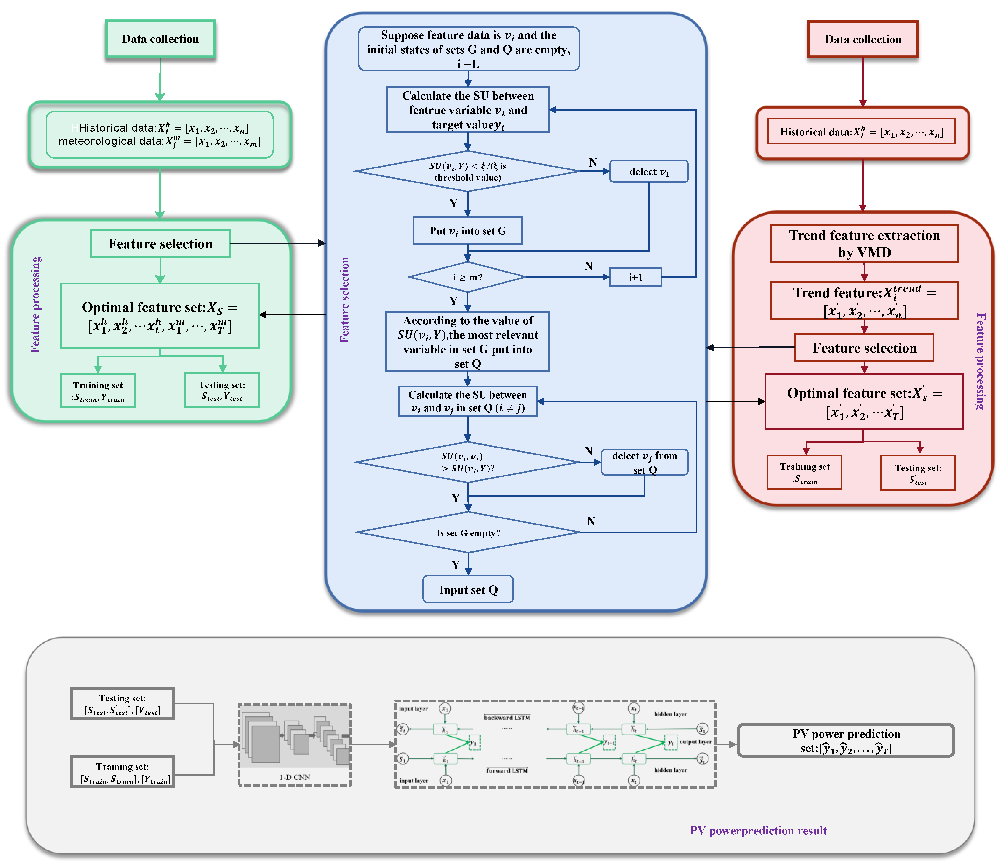
2. Framework of the Proposed Methodology

The hybrid model combined trend feature extraction and feature selection with BiLSTM for day-ahead PV power forecasting, and the proposed methodology was employed to predict PV power in Australia.

Figure 1 illustrates the general framework of the proposed methodology, and the procedures are as follows:

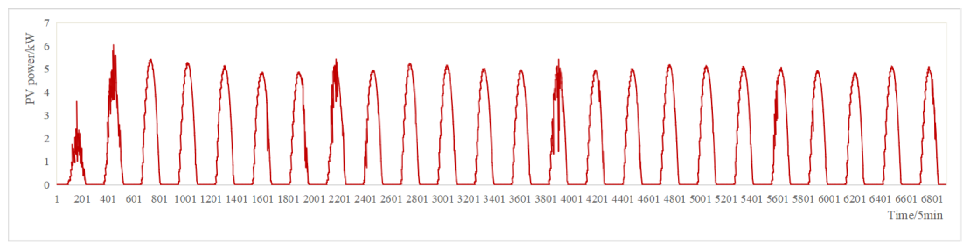
• Standard normalization and data procession of the original load data are required before performing trend feature extraction.
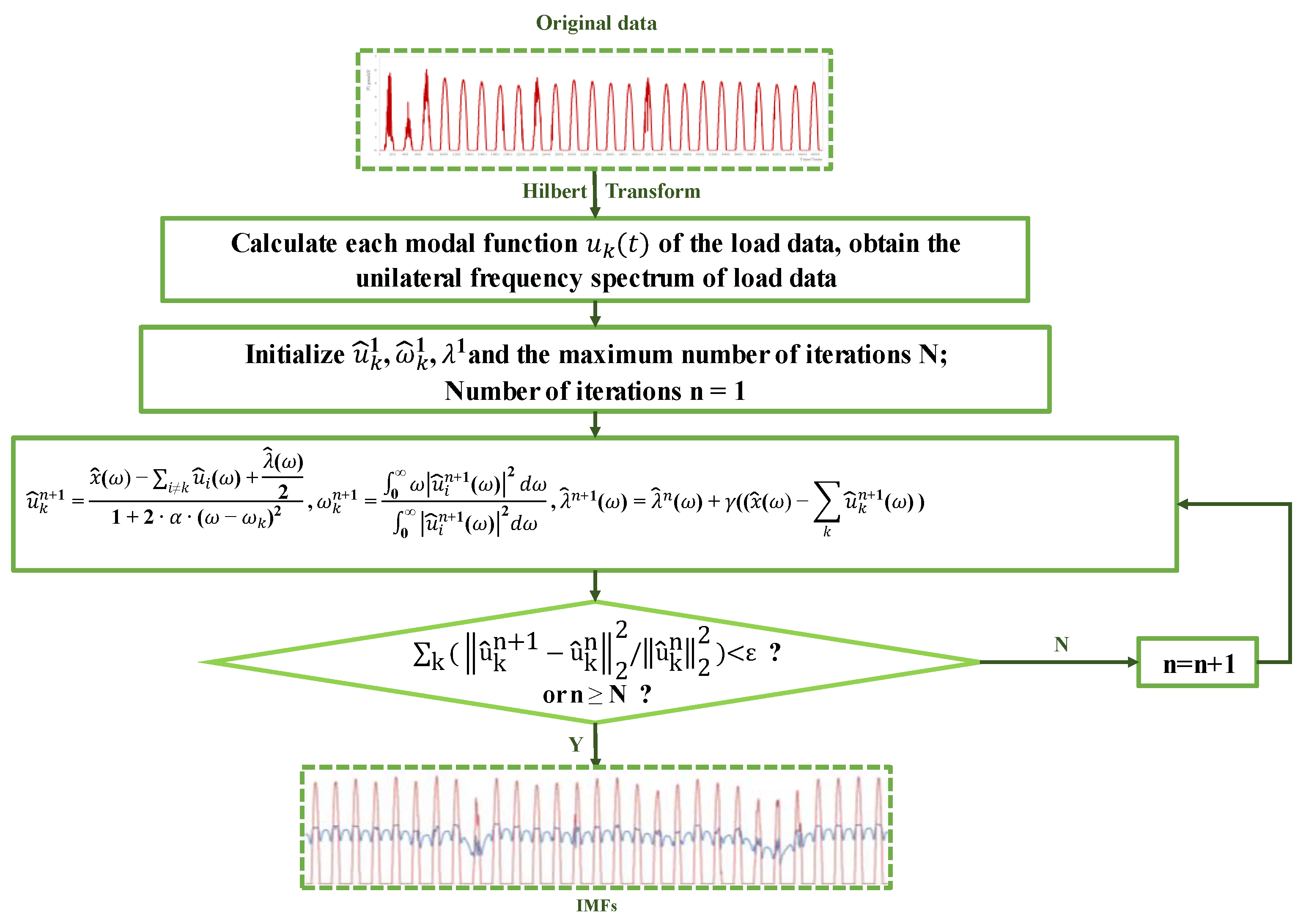
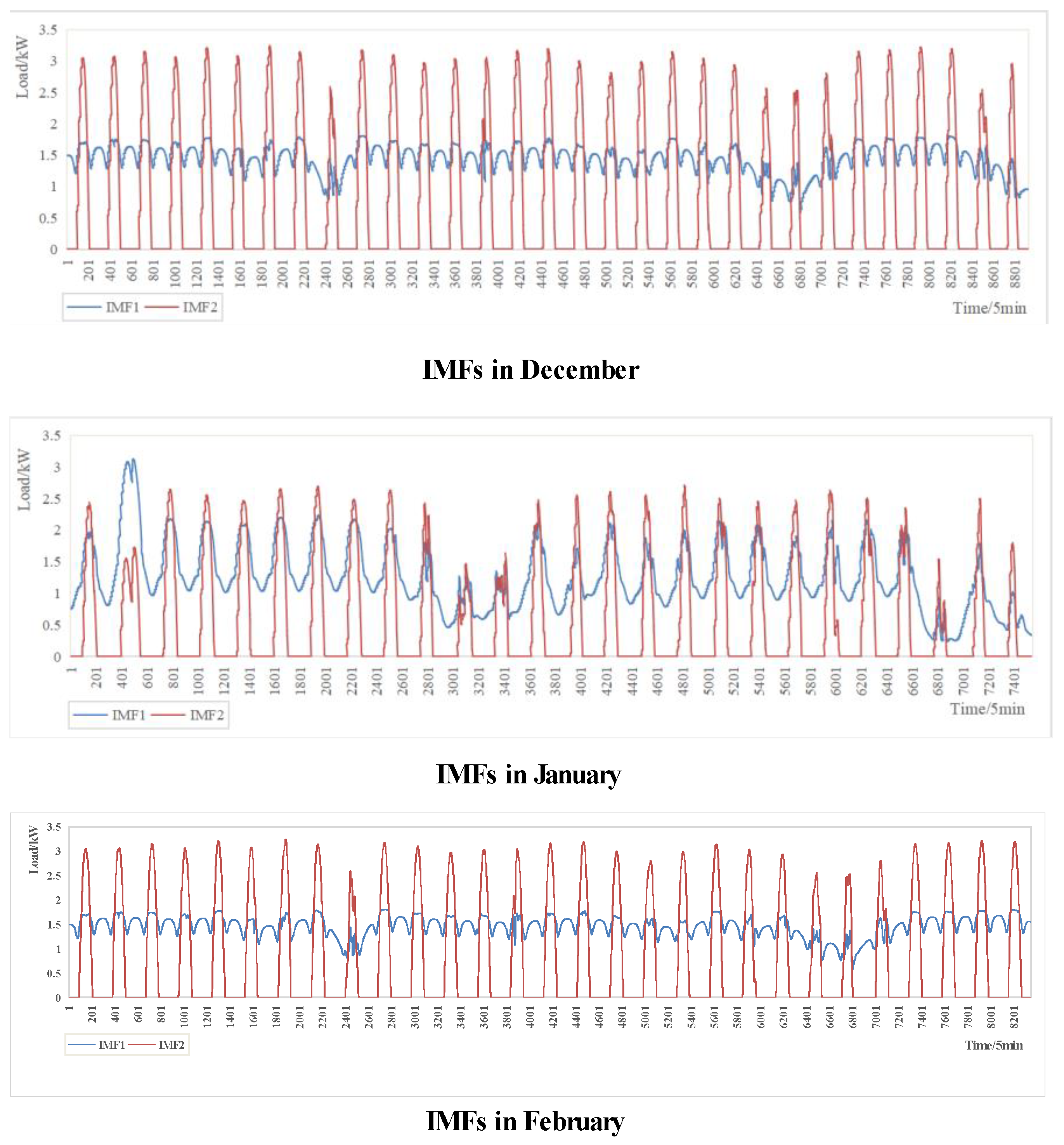
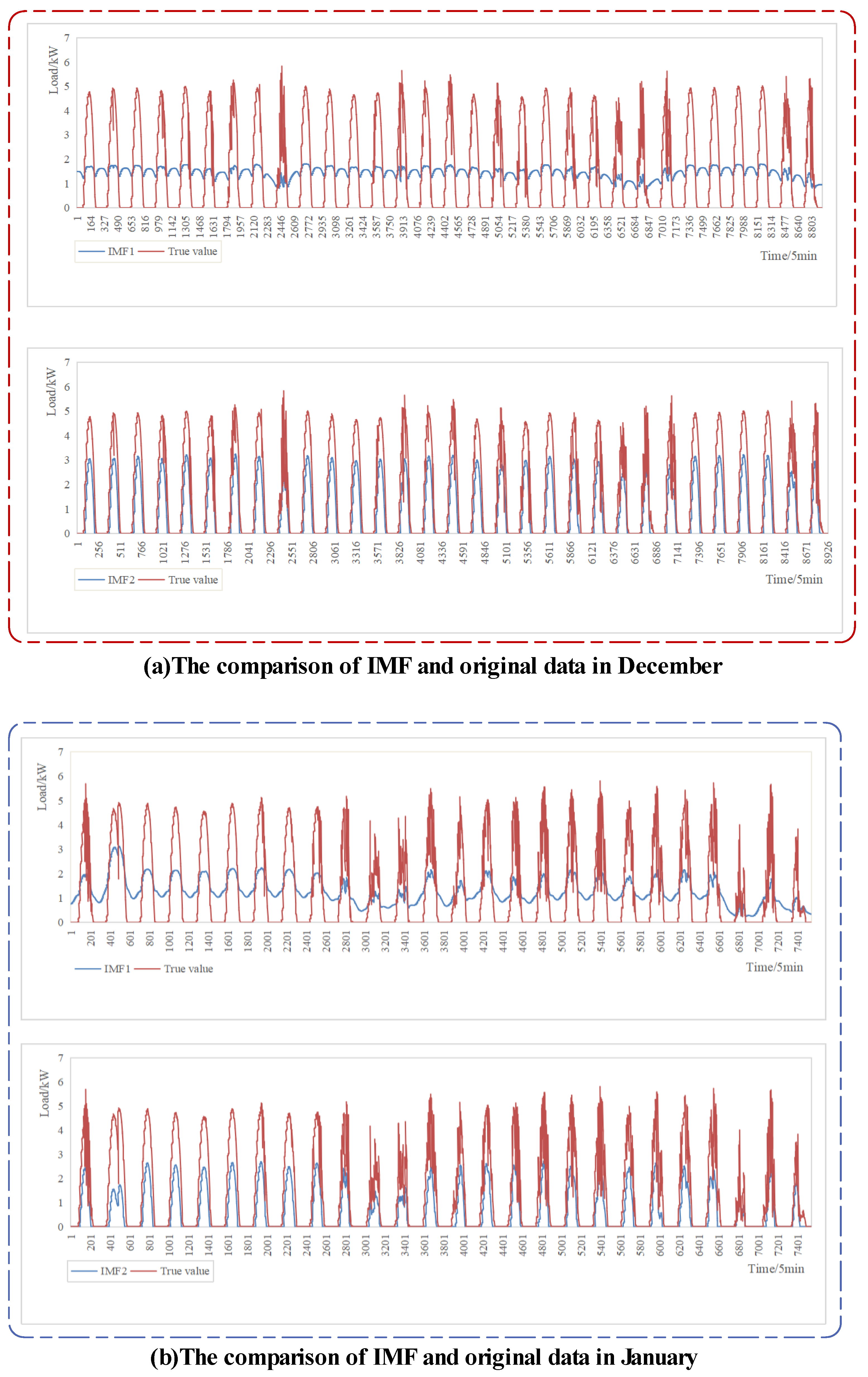
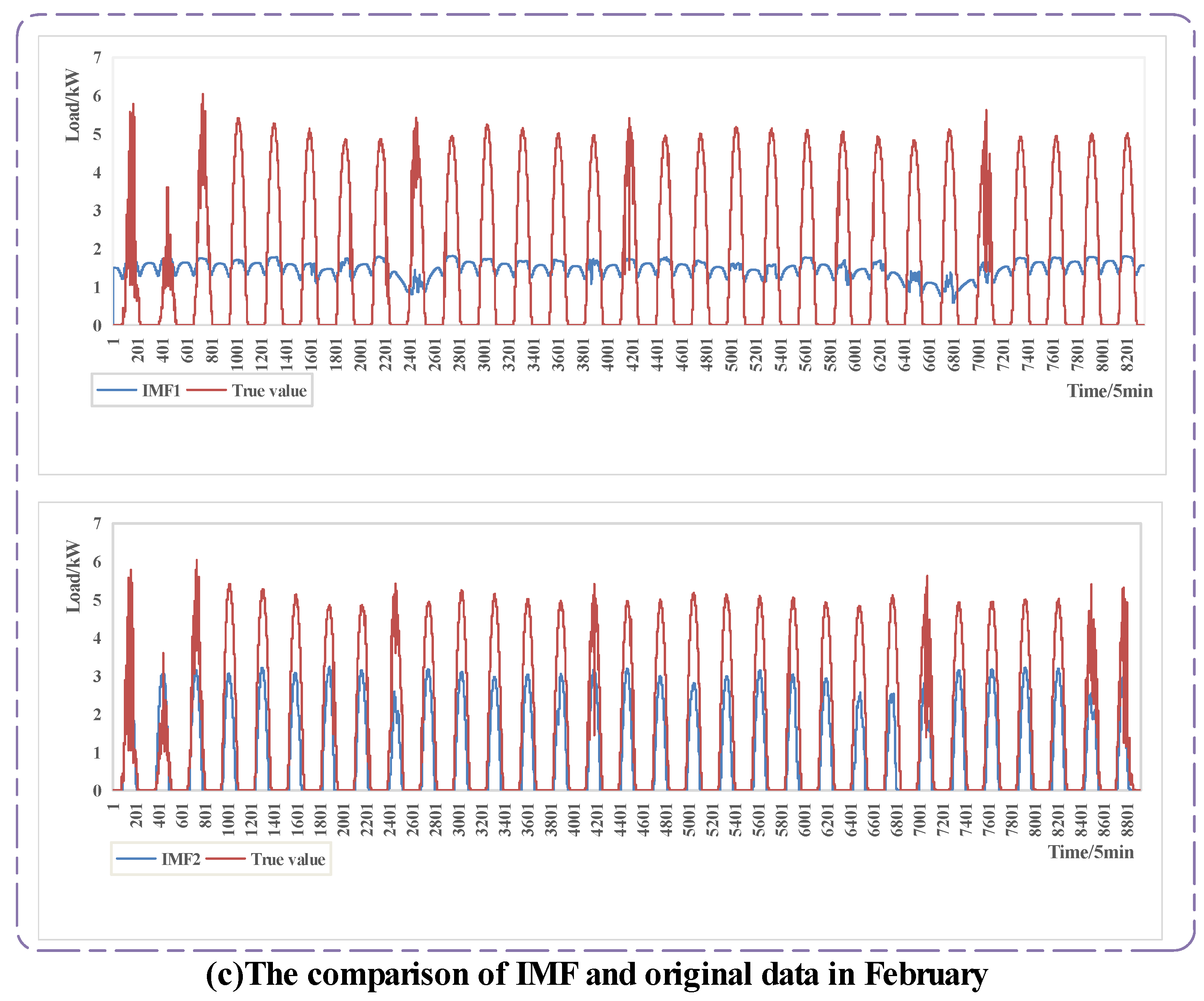
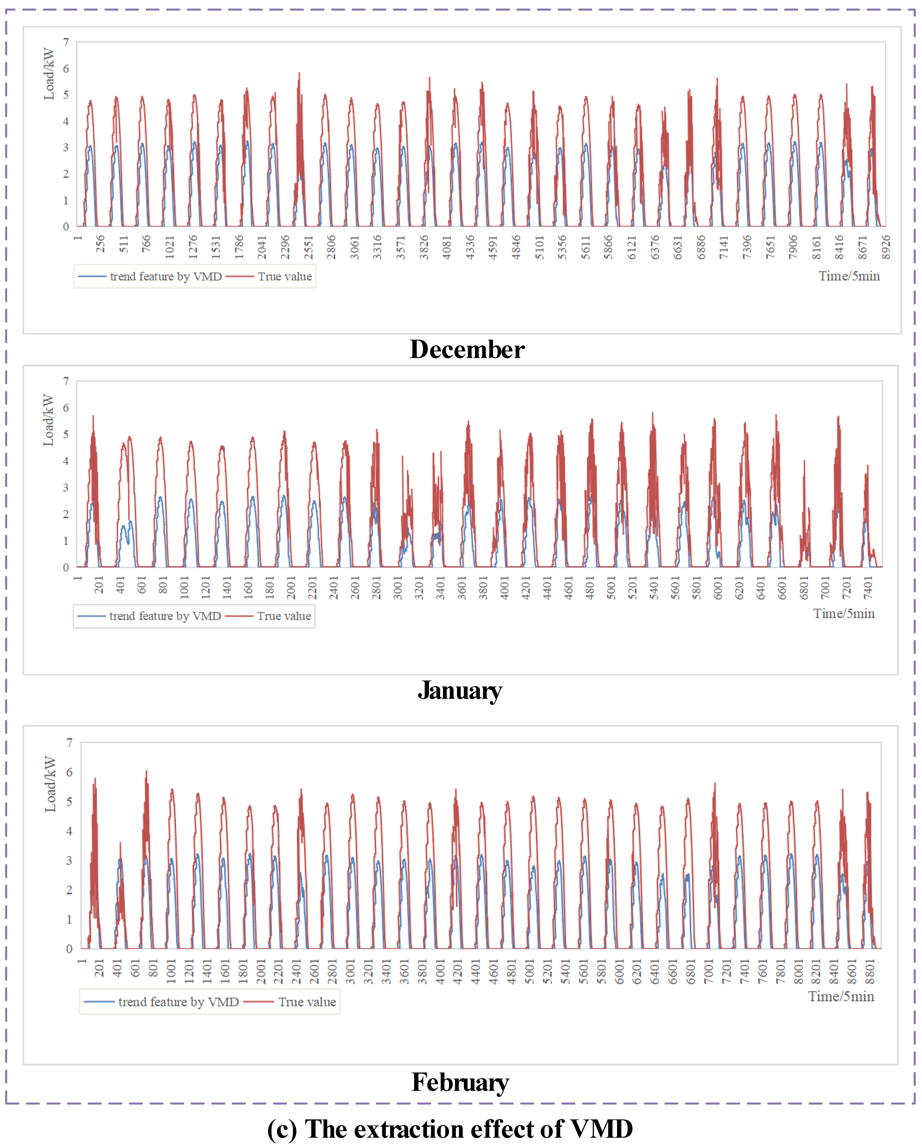
• The processed data are decomposed into multiple IMFs by VMD to extract the trend feature that can reflect the short-term effect of PV power.
• The optimal feature-sets of trend feature and the original data are selected by FCBF, and are then integrated as a new input-matrix.
• Finally, the optimal input-set is used in the standard BiLSTM model with a 1-D CNN layer to forecast the PV power.

Figure 1. Framework of proposed methodology.

Figure 1. Framework of proposed methodology.

3. Methodology

3.1. Variational Mode Decomposition (VMD)

The VMD algorithm considers that successive data are composed of sub-series with different frequencies. The essence of the VMD algorithm is to decompose the successive data into sub-modes that have different center frequencies [31]. PV power may be composed of a trend feature and noise, so the trend feature can be extracted from the PV power by using the VMD algorithm. The flow of the VMD algorithm consisted of the following steps.

Step 1: the number of modes ($K$) to be decomposed need to be preset, and then the original PV power $x(t)$ is decomposed into k modes $u_k$, ($k=1,2,...,K$). The original data of each mode is obtained by Hilbert transform. By adding an exponential term to adjust the estimated central spectrum, the spectrum of each intrinsic mode function (IMF) is modulated to the corresponding fundamental-frequency-band. The estimated bandwidth corresponding to each IMF is obtained by calculating the norm of the gradient square (L2) of the demodulated signal. The expression is as follows:

$$\begin{array}{l}\underset{\left\{u_k\right\},\left\{{\omega }_k\right\}}{\min }\left\{{\displaystyle {\sum }_k{\Vert {\partial }_t[\delta (t)+\frac{j}{\pi t}\ast u_k(t)]e^{-j{\omega }_{k}t}\Vert }_2^2}\right\}\\ s.t.{\displaystyle \sum _k{u}_k=x(t)}\end{array}$$

(1)

where K is the number of modes to be decomposed, $u_k$ is the k-th decomposed IMF of the original data, ${\omega }_k$ is the k-th center frequency, ${\partial }_t$ is the partial derivative of the function to time t, $\delta (t)$ is the Dirac distribution function, j represents an imaginary unit, and “*” represents convolution. In the constraint condition of the above Equation (1), X(t) represents the original data to be decomposed. In addition, $\left\{u_k\right\}=\{u_1,u_2,...,u_K\}$ is a collection of all modes, $\left\{{\omega }_k\right\}=\{{\omega }_1,{\omega }_2,...,{\omega }_K\}$ is a set of center frequencies of each mode, and ${\displaystyle \sum _k*}={\displaystyle \sum _{k=1}^K*}$ is the sum of modes.

Step 2: Using a quadratic penalty term and Lagrange multiplication operator, the constrained problem is transformed into an unconstrained problem. The quadratic penalty item is used to ensure that the key information of the PV data is not lost in the decomposition process. The purpose of the Lagrange multiplication operator is to force the constraints to have a certain degree of strictness.

The extended Lagrange expression is as follows:

$$L(\{u_k\},\{{\omega }_k\},\lambda )=\alpha {\displaystyle \sum _k{\Vert {\partial }_t[\delta (t)+\frac{j}{\pi t}\ast u_k(t)]e^{-j{\omega }_{k}t}\Vert }_2^2}+{\Vert x(t)-{\displaystyle \sum _k{u}_k(t)}\Vert }_2^2+\langle \lambda (t),x(t)-{\displaystyle \sum _k{u}_k(t)}\rangle$$

(2)

where $\alpha$ is the secondary penalty factor and $\lambda (t)$ is the Lagrangian multiplication operator.

An alternating direction method of multipliers (ADMM) is used to update $u_k^{n+1},{\omega }_k^{n+1}$ and ${\lambda }_k^{n+1}$ alternately, so that the minimization problem in Equation (1) is transformed into finding the Saddle point of extended Equation (2) in the iterative sub-optimization series. The calculation equation for updating $u_k^{n+1}$ can be expressed as follows:

$$u_k^{n+1}=\underset{u_k\in X}{\arg \min }\left\{\alpha {\displaystyle \sum _k{\Vert {\partial }_t[\delta (t)+\frac{j}{\pi t}\ast u_k(t)]e^{-j{\omega }_{k}t}\Vert }_2^2}+{\Vert x(t)-{\displaystyle \sum _i{u}_i(t)}+\frac{\lambda (t)}{2}\Vert }_2^2\right\}$$

(3)

where ${\omega }_k$ is equivalent to ${\omega }_k^{n+1}$, and ${\displaystyle \sum _i{u}_i^n}$ is equivalent to ${\displaystyle \sum _i{u}_i^{n+1}}$.

Step 3: By using the Parseval Fourier equidistant transform, Equation (3) is transformed from a time domain to a frequency domain, and the expression of each mode in the frequency domain is as follows:

$${\tilde{u}}_k^{n+1}=\frac{\widehat{x}(\omega )-{\displaystyle \sum _{i\ne k}{\widehat{u}}_i(\omega )+\frac{\widehat{\lambda }(\omega )}{2}}}{1+2\cdot \alpha \cdot {(\omega -{\omega }_k)}^2}$$

(4)

To obtain the updated center frequency ${\tilde{\lambda }}_k^{n+1}$ of each mode ${\omega }_k^{n+1}$, it is also necessary to transform the problem of solving the center frequency to the frequency domain to obtain the expression of update ${\omega }_k^{n+1}$. The expression is as follows:

$${\omega }_k^{n+1}=\frac{{{\displaystyle {\int }_0^{\infty }\omega \left|{\widehat{u}}_i^{n+1}(\omega )\right|}}^{2}d\omega }{{{\displaystyle {\int }_0^{\infty }\left|{\widehat{u}}_i^{n+1}(\omega )\right|}}^{2}d\omega }$$

(5)

$${\widehat{\lambda }}^{n+1}(\omega )={\widehat{\lambda }}^n(\omega )+\gamma ((\widehat{x}(\omega )-{\displaystyle \sum _k{\widehat{u}}_k^{n+1}(\omega ))}$$

(6)

In Equation (5), ${\omega }_k^{n+1}$ is the center frequency of the k-th IMF, and $u_i^{n+1}(\omega )$ is equivalent to the Wiener filter of current remaining amount $\widehat{x}(\omega )-{\displaystyle \sum _{i\ne k}{\widehat{u}}_i^{n+1}(\omega )}$. Equation (6) is used for updating the Lagrange factor ${\widehat{\lambda }}^{n+1}(\omega )$. It has the characteristics of a Wiener filter structure, which directly updates the mode in the frequency domain.

Figure 2 shows the flowchart of the VMD algorithm where $\forall \epsilon >0$.

3.2. Fast Correlation-Based Filter (FCBF)

The FCBF algorithm takes symmetrical uncertainty (SU) as the measurement index to define whether a feature is related to the target data or whether it is a redundant feature. Assuming that the target quantity is, $Y=[y_1,y_2,...,y_j]$ the historical PV power and meteorological data are $X=[x_1,x_2,...,x_i]$

$$H(X)=-{\displaystyle \sum _{i}P(x_i){\log }_{2}P(x_i)}$$

(7)

$$I(X;Y)=H(X)-H(X|Y)$$

(8)

where $H(X)$ is the information entropy of variable $X$, $H(X|Y)$ represents the conditional entropy of variables $X$ under the condition of variables $Y$, $I(X;Y)$ represents the mutual information that the information entropy of variables $X$ decreases after random variables $Y$ are observed.

$P(x_i)$ and $P(y_j)$ are the probabilities of variables $X=x_i$ and $Y=y_j$ respectively. $P(x_i|y_j)$ is the rate of variable $X=x_i$ under the condition of random variable $Y=y_j$. However, the size of $I(X;Y)$ is affected by the variables, values and units. In order to eliminate this influence, normalized mutual information $SU$ is used to represent the correlation between variables $X$ and $Y$. $SU$ is defined by Equation (9):

$$SU(X,Y)=2[I(X;Y)/(H(X)+H(Y))]$$

(9)

It can be seen from (9) that the value of $SU(X,Y)$ is between [0, 1]. The greater the value, the greater the correlation between the two random variables. When $SU(X,Y)=0$, this means that the two random variables $X$ and $Y$ are not related. On the contrary, when $SU(X,Y)=1$, this means that the random variables $X$ and $Y$ are completely correlated.

The steps of feature selection of original data using the FCBF algorithm are as follows.

• Delete the feature that is less relevant to the target variable. Take the i-th feature ($v_i$) in the original data as variable $X$ and the target variable $Y$ as category C. Calculate the $SU(v_i,Y)$ of each input feature and $Y$. If $SU(v_i,Y)<\xi$ ($\xi$ is threshold), delete the variable $v_i$, and put the retained feature variables into the set G with an empty initial state.
• Analyze redundancy between feature variables. The feature variables in set G are arranged according to the correlation degree of $SU(v_i,Y)$ from large to small. Take the feature variable $v_i$ with the largest correlation and put it into set Q with empty initial state, and then calculate the $SU(v_i,v_j)$ between the remaining characteristic variables $v_j$ in set G and $v_i$. If $SU(v_i,v_j)>SU(v_i,Y)$, remove the variable $v_j$ from set G.
• Return to step 2 and repeat the operation to finally obtain the optimized input feature set Q.

3.3. Improved BiLSTM Short-Term PV Power Forecasting Model

Long short-term memory (LSTM) greatly improves the model’s ability to store historical load data by adding storage units and gate mechanisms. The LSTM model consists of a series of identical modules [32]. LSTM is mainly composed of three gate structures, including the input gate, memory gate and output gate. The input gate is used to input the historical PV power, the memory gate is used to retain the useful information of historical data, irrelevant information is filtered, and the output gate is used to control the predicted PV power [33].

The bidirectional long short-term memory model (BiLSTM) is actually a deformation of LSTM. It is a two-direction LSTM neural network combined with an LSTM neural network that moves from the beginning, and a LSTM neural network that moves from the end of the load data to the beginning. The biggest difference between BiLSTM and LSTM is that the hidden state $H_t$ of BiLSTM at time $t$ includes the forward hidden state ${\overrightarrow{h}}_t$ and the backward hidden state ${\overleftarrow{h}}_t$. The relationships of ${\overrightarrow{h}}_t$ and ${\overleftarrow{h}}_t$ are as follows:

$${\overrightarrow{h}}_t=\overrightarrow{LSTM}(h_{t-1},x_t,c_{t-1}),t\in [1,T]$$

(10)

$${\overleftarrow{h}}_t=\overleftarrow{LSTM}(h_{t+1},x_t,c_{t+1}),t\in [T,1]$$

(11)

$$H_t=[{\overrightarrow{h}}_t,{\overleftarrow{h}}_t]$$

(12)

where $x_t$ is the input of time t, $c_{t-1}$ is the memory component of time t − 1, and $c_{t+1}$ is the memory component of time t + 1.

The structure of BiLSTM and LSTM are presented in Figure 3. The improved BiLSTM is added to a convolution (CNN) layer in the standard BiLSTM. The newly added CNN layer can select the characteristics of the input data, reduce the redundancy of the input feature to a certain extent, and improve the accuracy of short-term PV forecasting.

4. Results and Discussion

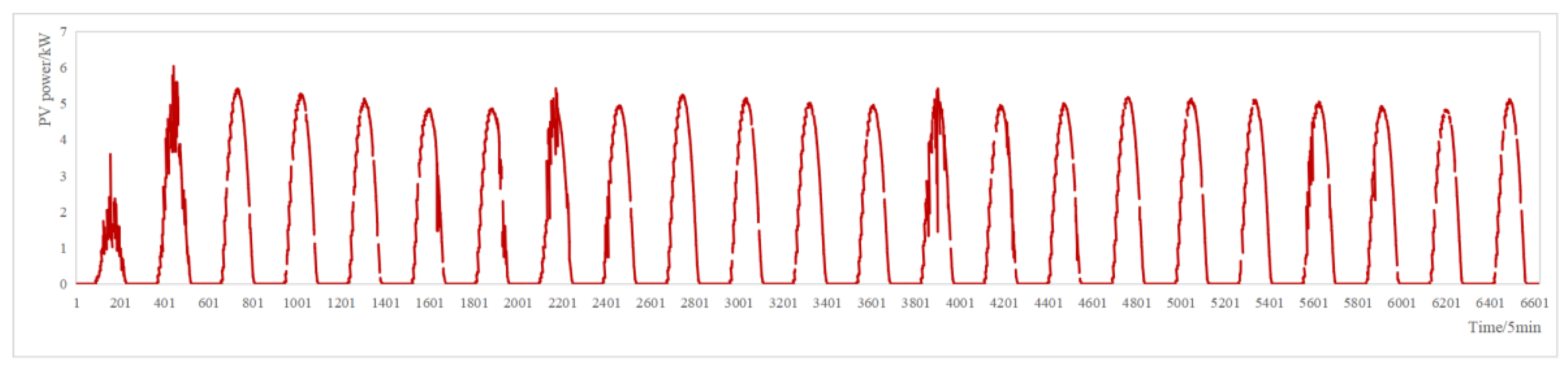
4.1. Data-Set

The DKASC Alice Springs PV system data were selected for experiments in this study [34]. There were 288 observation values every day (time interval is 5 min). The data included active power (kW), wind speed (m/s), weather temperature (${}^{°}\mathrm{C}$), weather relative humidity (%), global horizontal radiation ($w/m^2\times sr$), and diffuse horizontal radiation ($w/m^2\times sr$), among others, with 10 dimensions of data in total. The cases used in this paper can comprehensively and systematically evaluate the validity and usefulness of the proposed methodology.

PV power has a certain regularity, and the prediction model needs to learn from the historical PV power data to find its trend feature. The datasets included the real PV power from December 2021 to February 2022 and from June 2021 to August 2021. The data-set was continuous but there were some vacancy values. Before conducting experiments, the Lagrange interpolation method was used to process the original data and fill the vacancy values. The original data and processed data in February are shown in Figure 4 and Figure 5. Because of the large amount of data, the processed result only uses the data in February as an example.

Two sets of experiments were carried out to show the performance of the proposed model both in summer and winter, representing 1-day ahead and 3-day ahead short-term PV power forecasting. In 1-day ahead PV power forecasting, the training data accounted for 80% of the data-set, of which the training-set accounted for 80%, the verification-set accounted for 20%, and the rest of the data-set was the testing data; In 3-day ahead PV power forecasting, the training data accounted for 80% of the data-set, of which the training set accounted for 80%, the verification set accounted for 20%, and the rest of the data set was the testing data.

Before carrying out the experiments, original data were standardized and normalized. The equation for normalization is as follows:

$$x_g=\frac{x-x_{\min }}{x_{\max }-x_{\min }}$$

(13)

where $x$ is the original PV power data, $x_{\mathrm{m}ax}$ and $x_{\min }$ are the maximum and minimum of the data, and $x_g$ is the normalized data. From Equation (13), $x_g$ can be obtained in the interval [0, 1].

4.2. Evaluation Criteria

In order to evaluate the prediction effect of the fusion model for PV power prediction, the mean absolute error (MAE), root mean square error (RMSE) and mean absolute percentage error (MAPE) were applied as evaluation indexes, which can be described as:

$$MAE=\frac{1}{n}{\displaystyle \sum _{i=1}^n\left|{\widehat{y}}_i-y_i\right|}$$

(14)

$$RMSE=\sqrt{\frac{1}{n}{\displaystyle \sum _{i=1}^n{(y_i-{\widehat{y}}_i)}^2}}$$

(15)

$$MAPE=\frac{1}{n}{\displaystyle \sum _{t=1}^n\frac{\left|{\widehat{y}}_i-y_i\right|}{{\widehat{y}}_i}}\times 100\%$$

(16)

where, ${\widehat{y}}_i$ is the actual value of PV data, $y_i$ is the predicted value, and $n$ is the number of testing points.

4.3. Simulation Analysis

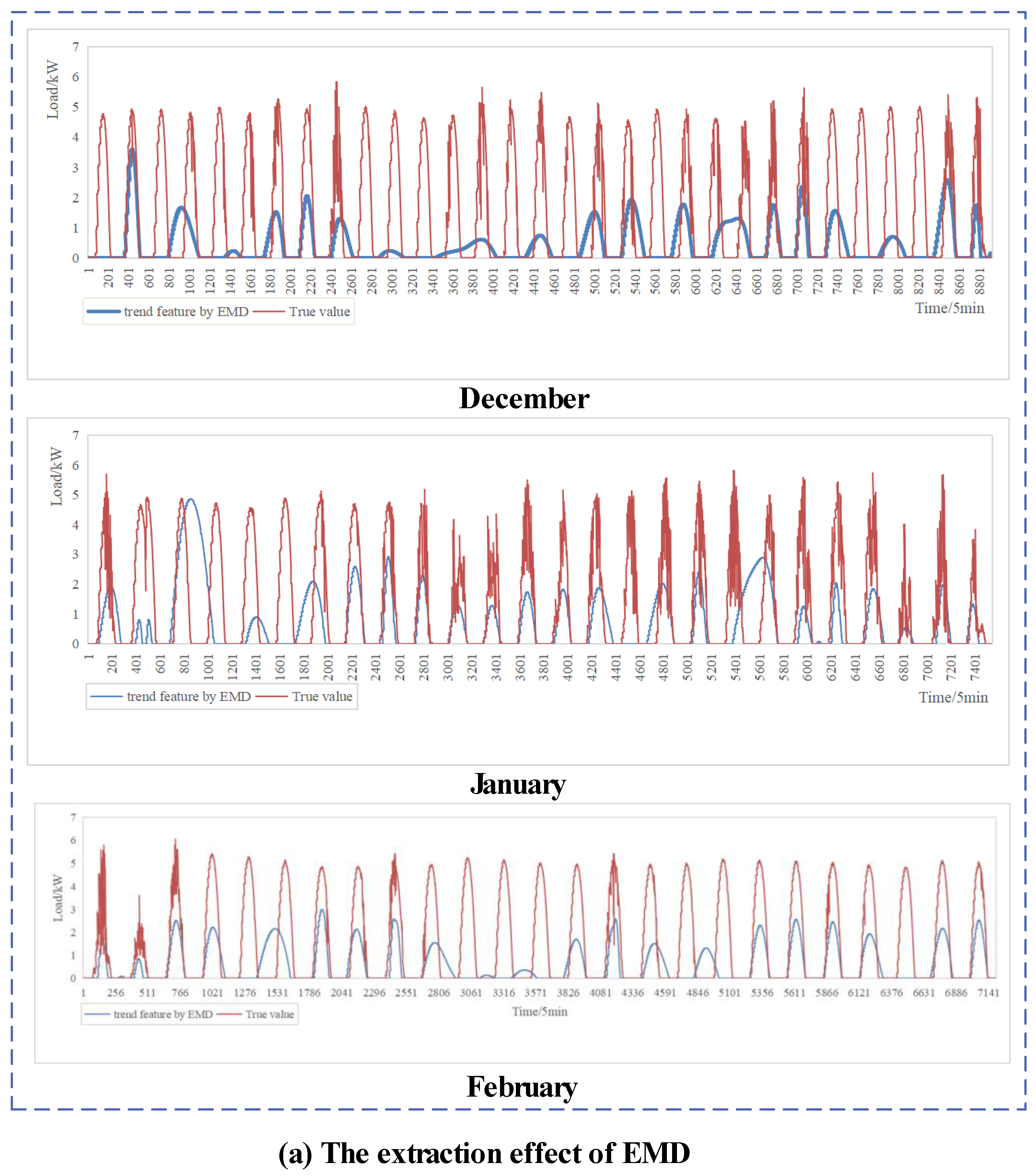
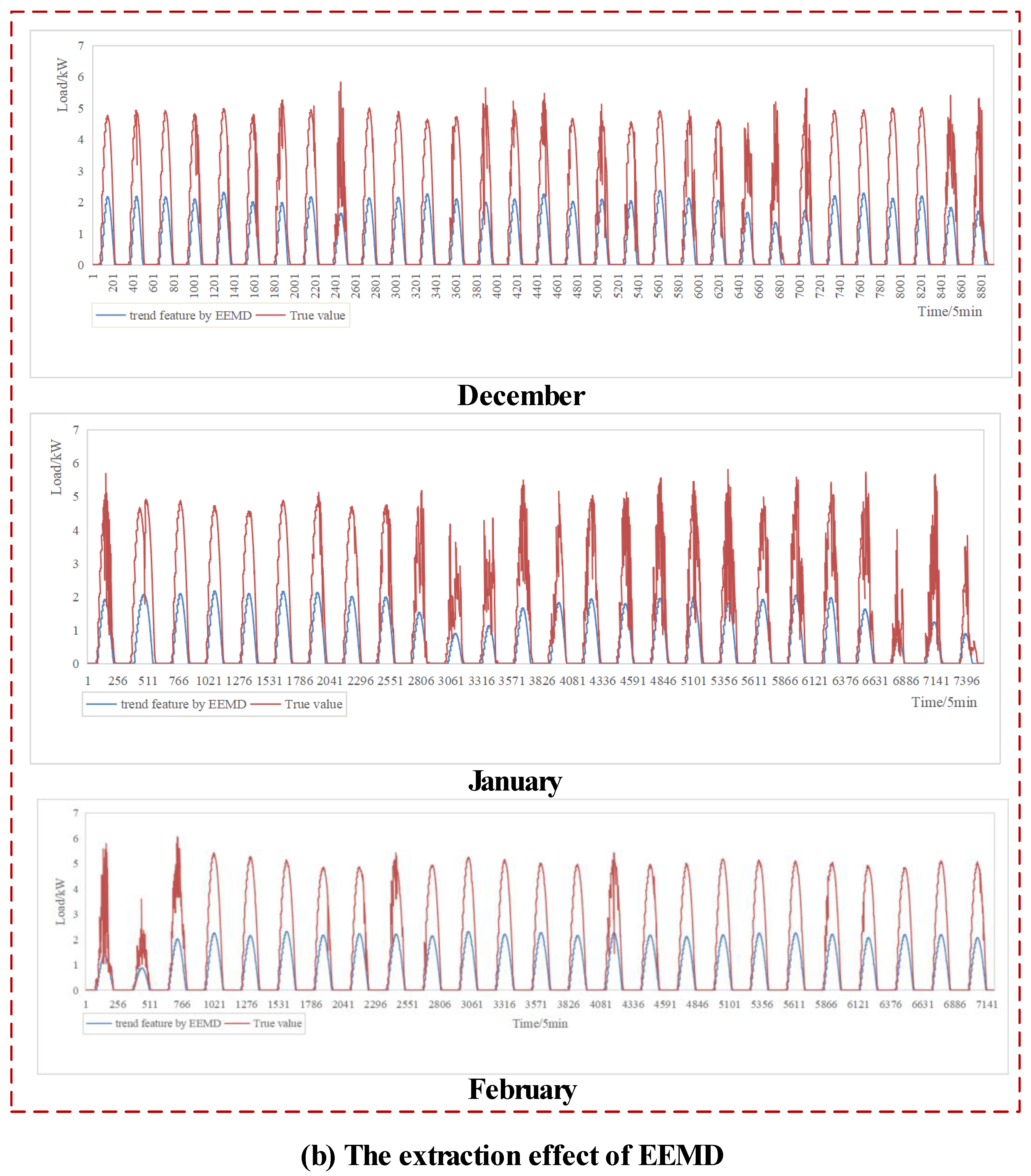
4.3.1. Comparison of Different Trend Feature Extraction Models

Different trend feature extraction models were compared taking the data-set in summer as an example for verifying the effectiveness and excellence of the variational mode decomposition (VMD). After many experiments, it was found that if the number of modes decomposed by VMD was too large, the essential information of intrinsic mode functions (IMFs) was lost, which was manifested in the trend feature that did not fit the change of the original load data. When the number of decomposition modes was 2, the trend feature extraction performance of VMD model was best. It can be concluded that VMD can accurately separate noise and trend variables without losing significant information of photovoltaic (PV) power. The original data with a wide time range included three months of PV power. In order to more intuitively reveal the extraction effect of the trend feature, Figure 6, Figure 7 and Figure 8 shows the original data in three groups. The actual extraction process was carried out with continuous original data. Since the research direction of this paper was short-term PV power forecasting (time interval of 5 min), the trend feature should be extracted from recent PV power. After many experiments, the trend feature selected from the PV power in the same season was found to be most suitable. All IMFs of original data were decomposed by VMD and their comparison with original data are shown in Figure 6 and Figure 7. From Figure 6, in addition to the IMF, which reflects the trend of PV power, there is also certain high-frequency IMF in the original data. IMF1 may be generated by the equipment measuring PV power during the collection process, which affects the performance of the prediction model. From the comparison between each IMF and the original data in Figure 7, it can be seen that IMF1 has almost no relationship with the change of the original data. Only IMF2 is closest to the pattern of the original data. Therefore, IMF2 was selected as the trend feature.

The VMD model was compared with more common trend extraction algorithms (such as empirical mode decomposition (EMD), and ensemble empirical mode decomposition (EEMD)). These models took the real PV power of a PV power station in Australia as the input, and checked the trend feature extraction effect of each model by observing the fit between the trend feature and true data. Symmetrical uncertainty (SU) was also used to measure the correlation between the trend feature and true values. The comparison results between trend variables extracted by each model and the original data are shown in Figure 8. The operation time and SU of each model are given in

Table 1. SU and operation time of different trend feature extraction algorithms.

Algorithm	SU	Operation Time(s)
EMD	0.71	180 s
EEMD	0.72	30 s
VMD	0.73	6 s

.

From Figure 8 and Table 1, the trend feature extracted by VMD better fit the PV power, the operation speed of VMD was the fastest, and it had the best correlation between the extracted trend feature and the original data. The trend extraction effect of EEMD was good, and almost consistent with the change of PV power. However, the fitting degree of the trend feature extracted by EEMD in amplitude was not as good as that of VMD. The VMD model used in this paper fitted the load change of the original data both in amplitude and tendency.

4.3.2. Selection of the Models’ Input-Set

During the experiments, this study took 17 dimensions of features which included various meteorological information, historical photovoltaic (PV) power, and trend features. The target value was the PV power on the prediction day, and the fast correlation-based filter (FCBF) algorithm was used to find the most appropriate input-set for all short-term PV power forecasting models. Based on experience summary and driven by prediction error, the optimal input-set selected by the FCBF algorithm is shown in

Table 2. Feature selection results.

Number	Input Variable
0	d-1 PV Power
1	Weather Relative Humidity
2	Global Horizontal Radiation
3	Weather Daily Rainfall
4	Radiation Global Tilted
5	Trend feature

d-1 is the day before the target day d.

.

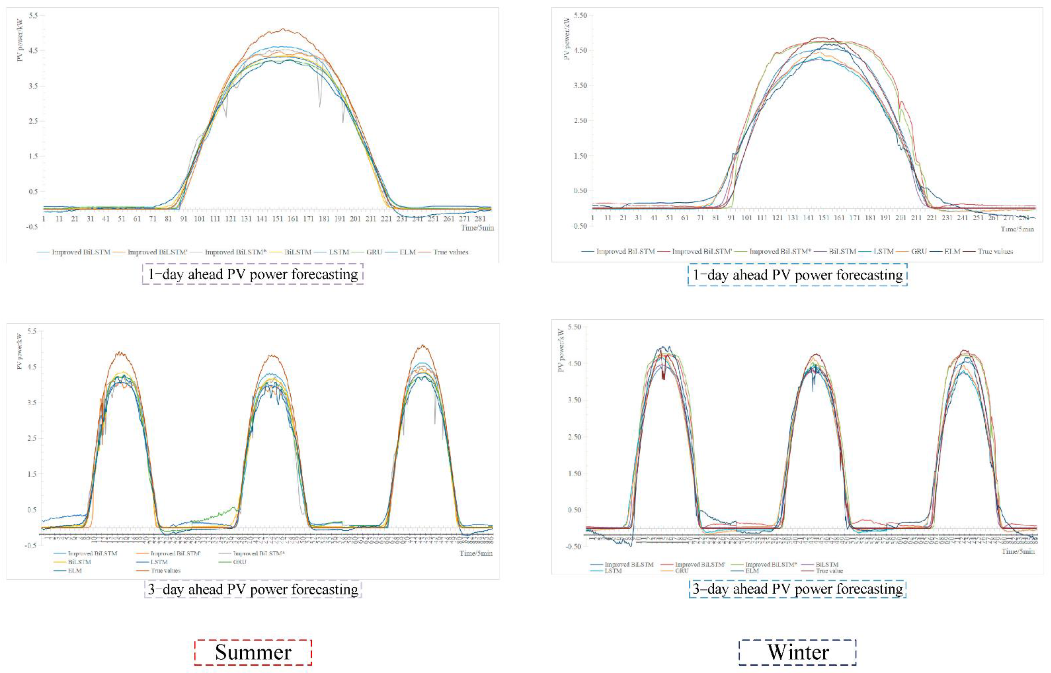
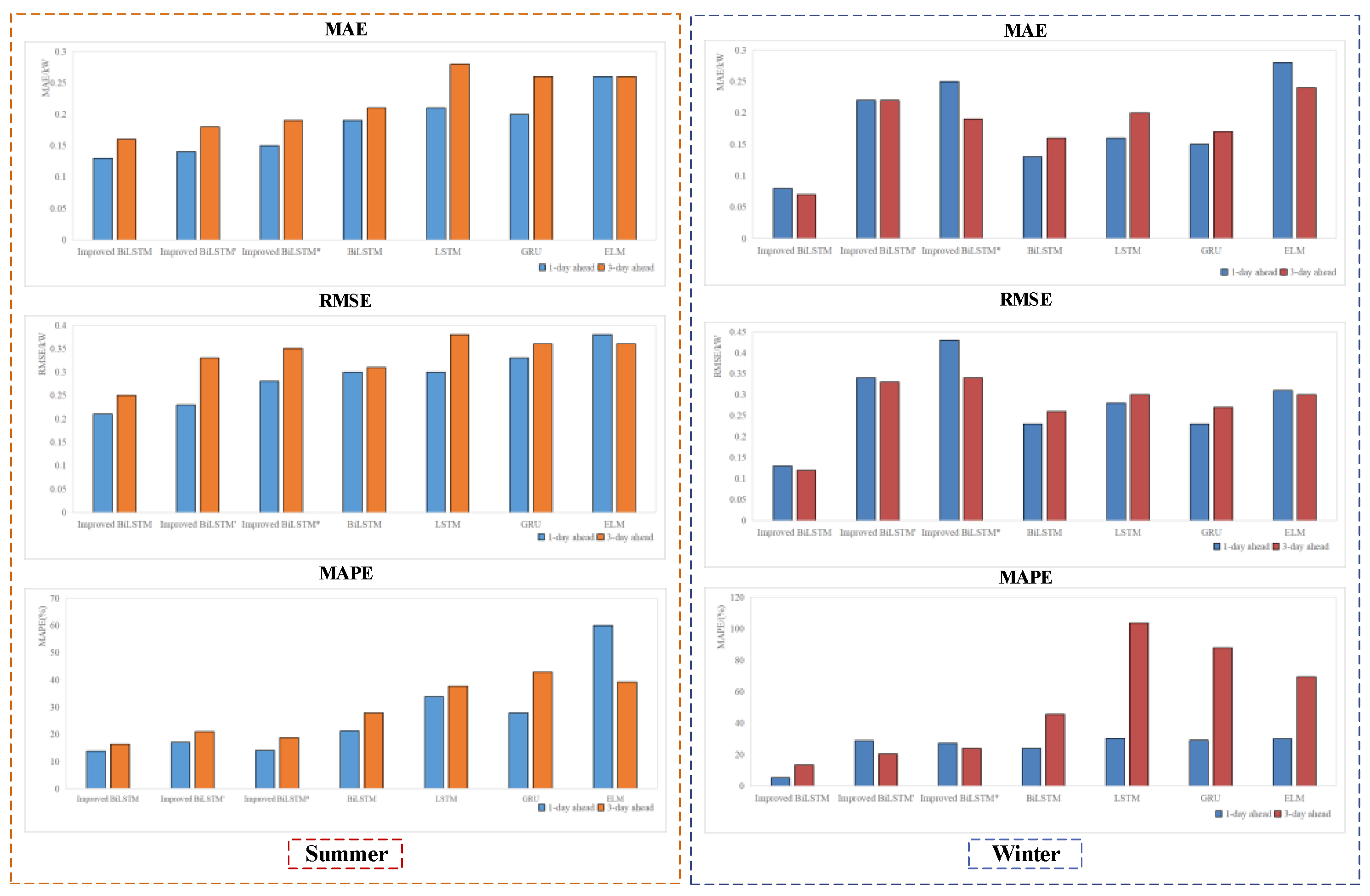
4.3.3. Comparison and Analysis of Prediction Results

Different short-term photovoltaic (PV) power forecasting models were introduced to predict PV power in different horizons. The results of the improved bidirectional long short-term memory (BiLSTM) model and extreme learning machine (ELM), BiLSTM, long short-term memory (LSTM) and gate recurrent unit (GRU) models were compared with 1-day ahead and 3-day ahead horizon for short-term PV power prediction. All experiments were repeated more than 10 times, and results averaged in multiple repeated runs.

The historical data of PV power between June 2021 and August 2021 (Winter), and between December 2021 and February 2022 (Summer), were used to predict PV daily power 1-day ahead (288 points in total) and 3-days ahead (288 $\times$ 3 points in total), respectively. Short-term PV power prediction results of different models are shown in Figure 9. According to the evaluation measures of mean absolute error (MAE), root mean square error (RMSE) and mean absolute percentage error (MAPE), short-term PV power prediction results of different forecasting models are reported in

Table 3. The MAE and RMSE of different forecasting models in Summer.

Model	MAE (kW)		RMSE (kW)		MAPE (%)
	1-Day Ahead	3-Day Ahead	1-Day Ahead	3-Day Ahead	1-Day Ahead	3-Day Ahead
Improved BiLSTM	0.13	0.16	0.21	0.25	13.84	16.33
Improved BiLSTM ’	0.14	0.18	0.23	0.33	17.08	21.00
Improved BiLSTM *	0.15	0.19	0.28	0.35	14.07	18.69
BiLSTM	0.19	0.21	0.30	0.31	21.17	27.82
LSTM	0.21	0.28	0.30	0.38	33.84	37.71
GRU	0.20	0.26	0.33	0.36	27.82	42.8
ELM	0.26	0.26	0.38	0.36	59.9	39.24

and

Table 4. MAE and RMSE of different forecasting models in Winter.

Model	MAE (kW)		RMSE (kW)		MAPE (%)
	1-Day Ahead	3-Day Ahead	1-Day Ahead	3-Day Ahead	1-Day Ahead	3-Day Ahead
Improved BiLSTM	0.08	0.07	0.13	0.12	5.21	13.28
Improved BiLSTM ’	0.22	0.22	0.34	0.33	28.9	20.26
Improved BiLSTM *	0.25	0.19	0.43	0.34	27.26	23.89
BiLSTM	0.13	0.16	0.23	0.26	24.00	45.48
LSTM	0.16	0.20	0.28	0.30	30.36	103.55
GRU	0.15	0.17	0.23	0.27	29.10	87.73

In Figure 9 and Figure 10 and Table 3 and Table 4, the PV power forecasting model with ’ indicates that there is no trend feature added to the input-set of the model. The model with * indicates that this PV forecasting model does not undergo feature selection.

and in Figure 10. From the experimental results, the 1-day ahead and 3-day ahead prediction results both in summer and winter of the proposed methodology were the closest to the true values, and the prediction performance of this model was the best of the five models. The comprehensive error index analysis results in Table 3 and Table 4 and in Figure 10 show that the MAE, RMSE and MAPE of the improved BiLSTM model are the lowest, indicating that the prediction performance of this model was the best among the five load forecasting models. In summer, if the trend feature extraction was added to the forecasting model, for 1-day ahead forecasting, MAE, RMSE and MAPE of the model was reduced 7.69, 13.0 and 19.0% respectively. For 3-day ahead PV power forecasting, the MAE, RMSE and MAPE of the model were reduced 11.1, 24.2 and 22.23%, respectively. If feature selection was added to the model, for 1-day ahead forecasting, the MAE, RMSE and MAPE of the model were decreased by 13.3, 28.6 and 1.63%, respectively, while for 3-day ahead forecasting, the MAE, RMSE and MAPE of the model were reduced by 15.8, 28.6 and 25.95%, respectively. In winter, the prediction effect of this model was more effective, and the MAPE of 1-day ahead prediction could reach 5.21%. The prediction precision in winter was better than that in summer, which may be because the change of weather in winter is less intense than that in summer, and the feature of PV power is more stable, which lead to higher accuracy.

From the Figure 9, the error between the predicted value and the true value is large in the high radiation situations. It may be affected by the feature of radiation-diffusion-limited, which tends to be stable at the peak of PV power, resulting in the predicted values being lower than the true values.

The experiments were conducted using a personal computer with a Python 3.9, 64-bit operating system, 16.00 GB of RAM, and Intel(R) Core(TM) i7-10510U CPU @ 1.80GHz 2.30 GHz. The performance of the improved BiLSTM model based on trend feature extraction and FCBF feature selection was improved, mainly as reflected in the MAE, RMSE and MAPE of forecasting results of the model in summer and winter. Even if the improved BiLSTM model did not carry out feature selection and trend feature extraction, its prediction error was still the lowest among all models in summer, indicating that the model was superior and has prospects in short-term PV power prediction. When feature selection was added to the model, the accuracy of both 1-day ahead prediction and 3-day ahead prediction was further improved which shows that feature selection cannot be ignored before prediction. In the experiment concerning the model’s trend feature input, the addition of the trend feature had a great effect on improvement of 3-day ahead prediction results. The trend feature provides the current effects of PV power change in the region, reducing the influence of outliers on the prediction model, improving the performance of the prediction model and improving the accuracy of load forecasting effectively. In general, the trend feature can account for the timing characteristics among PV power, and plays a great role in multi-day ahead PV power forecasting.

5. Conclusions

This article proposes an improved bidirectional long short-term memory (BiLSTM) model combined with trend feature extraction and feature selection for accurate short-term photovoltaic (PV) power forecasting. First, the original PV data is disintegrated to extract the trend feature of the PV power according to the principle of variable mode decomposition (VMD). Second, the optimal feature set is selected from trend feature, historical PV data and meteorological factors by a fast correlation-based filter (FCBF) algorithm, to lay a foundation for accurate short-term PV power prediction. Finally, the optimal feature set is applied to the improved BiLSTM model for training and testing. The proposed method was compared with the commonly used short-term forecasting models, such as BiLSTM, LSTM, GRU and ELM.

As illustrated in the simulation results in Table 1, Table 2, Table 3 and Table 4 and Figure 6, Figure 7, Figure 8, Figure 9 and Figure 10, the main conclusions are as:

• The collection process of PV power is complex, and the problem of outliers cannot be avoided. Therefore, the extraction of the trend feature with the VMD algorithm can reduce the prediction error caused by outliers and help the prediction model to fully learn the long-term time characteristics and short-term effects on PV power in this region.
• Reducing the error caused by high dimension of input variables using the FCBF algorithm to extract the optimal input feature set of the prediction model is conducive to improving the performance and efficiency of the prediction model.
• Compared with the commonly used short-term PV power forecasting model, the improved BiLSTM forecasting model can selectively combine historical information and trend information for PV power forecasting because of its unique structure.

In summary, this study starts from the time characteristics of PV data and considers the influence of relevant characteristics on the prediction results. Trend feature extraction and feature selection can provide high-quality load data for follow-up training of the prediction model, preventing the prediction model from learning from outliers and improving the prediction accuracy. With its special structure, the BiLSTM model can better extract long-term information in PV power. The performance of the proposed forecasting methodology is relatively stable and can provide an important reference for power grid planning, and power grid stable operation, and can assist technicians to reasonably arrange a dispatching plan of the power grid.

There are still many aspects that require further research.

(1)

Symmetrical loss function is used in this model, and the influence of asymmetric loss function on the prediction effect of the model is not considered. Next, we will conduct in-depth research in this direction.

(2)

An FCBF algorithm is used to extract the best feature set of PV prediction. In the FCBF algorithm, it is necessary to set the threshold of symmetrical uncertainty (SU) to extract features. A trial-and-error method was used to select the appropriate threshold in this paper. Next, we will try to use an optimization algorithm combined with the FCBF algorithm to select the optimal feature-set effectively.

References

1. Wu, X.; Lai, C.S.; Bai, C.; Lai, L.L.; Zhang, Q.; Liu, B. Optimal Kernel ELM and Variational Mode Decomposition for Probabilistic PV Power Prediction. Energies 2020, 13, 3592. [Google Scholar] [CrossRef]
2. Huang, C.-J.; Kuo, P.-H. Multiple-Input Deep Convolutional Neural Network Model for Short-Term Photovoltaic Power Forecasting. IEEE Access 2019, 7, 74822–74834. [Google Scholar] [CrossRef]
3. Lai, C.S.; Jia, Y.; Lai, L.L.; Xu, Z.; McCulloch, M.D.; Wong, K.P. A Comprehensive Review on Large-scale Photovoltaic System with Applications of Electrical Energy Storage. Renew. Sustain. Energy Rev. 2017, 78, 439–451. [Google Scholar] [CrossRef]
4. Kim, G.G.; Choi, J.H.; Park, S.Y.; Bhang, B.G.; Nam, W.J.; Cha, H.L.; Park, N.; Ahn, H.-K. Prediction Model for PV Performance with Correlation Analysis of Environmental Variables. IEEE J. Photovolt. 2019, 9, 832–841. [Google Scholar] [CrossRef]
5. Xie, C.; Wang, D.; Lai, C.S.; Wu, R.; Wu, X.; Lai, L.L. Optimal sizing of battery energy storage system in smart microgrid considering virtual energy storage system and high photovoltaic penetration. J. Clean. Prod. 2021, 281, 125308. [Google Scholar] [CrossRef]
6. Liu, C.; Li, M.; Yu, Y.; Wu, Z.; Gong, H.; Cheng, F. A Review of Multitemporal and Multispatial Scales Photovoltaic Forecasting Methods. IEEE Access 2022, 10, 35073–35093. [Google Scholar] [CrossRef]
7. Lai, C.S.; Zhong, C.; Pan, K.; Ng, W.W.Y.; Lai, L.L. A deep learning based hybrid method for hourly solar radiation forecasting. Expert Syst. Appl. 2021, 177, 114941. [Google Scholar] [CrossRef]
8. Xiao, B.; Zhang, S.; Chen, S.; Mo, S.; Wang, T.; Ouyang, Z. A Statistical Photovoltaic Power Forecast Model (SPF) based on Historical Power and Weather Data. In Proceedings of the 2021 IEEE 48th Photovoltaic Specialists Conference (PVSC), Fort Lauderdale, FL, USA, 20–25 June 2021; pp. 26–28. [Google Scholar] [CrossRef]
9. Huang, C.; Wang, L.; Lai, L.L. Data-Driven Short-Term Solar Irradiance Forecasting Based on Information of Neighboring Sites. IEEE Trans. Ind. Electron. 2019, 66, 9918–9927. [Google Scholar] [CrossRef]
10. Pan, K.; Zhen, Z.; Lai, C.S.; Xie, C.; Wang, D.; Zhao, Z.; Wu, X.; Tong, N.; Lai, L.L.; Hatziargyriou, N.D. A Novel Data-Driven Method for Behind-the-Meter Solar Generation Disaggregation with Cross-Iteration Refinement. IEEE Trans. Smart Grid 2022, 1. [Google Scholar] [CrossRef]
11. Li, Y.; Su, Y.; Shu, L. An ARMAX Model for Forecasting the Power Output of a Grid Connected Photovoltaic System. Renew. Energy 2014, 66, 78–89. [Google Scholar] [CrossRef]
12. Persson, C.; Bacher, P.; Shiga, T.; Madsen, H. Multi-site Solar Power Forecasting using Gradient boosted Regression Trees. Sol. Energy 2017, 150, 423–436. [Google Scholar] [CrossRef]
13. Li, Y.; Wang, Z.; Niu, J. Forecast of Power Generation for Grid-connected Photovoltaic System based on Grey Theory and Verification Model. In Proceedings of the 2013 Fourth International Conference on Intelligent Control and Information Processing (ICICIP), Beijing, China, 9–11 June 2013; pp. 129–133. [Google Scholar] [CrossRef]
14. Yazdanbaksh, O.; Krahn, A.; Dick, S. Predicting Solar Power Output using Complex Fuzzy Logic. In Proceedings of the 2013 Joint IFSA World Congress and NAFIPS Annual Meeting (IFSA/NAFIPS), Edmonton, AB, Canada, 24–28 June 2013; pp. 1243–1248. [Google Scholar] [CrossRef]
15. Ding, M.; Wang, L.; Bi, R. An ANN-based Approach for Forecasting the Power Output of Photovoltaic System. Procedia Environ. Sci. 2011, 11, 1308–1315. [Google Scholar] [CrossRef] [Green Version]
16. Kim, D.; Kwon, D.; Park, L.; Kim, J.; Cho, S. Multiscale LSTM-Based Deep Learning for Very-Short-Term Photovoltaic Power Generation Forecasting in Smart City Energy Management. IEEE Syst. J. 2020, 15, 346–354. [Google Scholar] [CrossRef]
17. Kartini, U.T.; Choiroh, U.N. Very Short Term Photovoltaic Power Generation Station Forecasting Based On Meteorology Using Hybrid model Decomposition-Deep Neural Network. In Proceedings of the 2021 Fourth International Conference on Vocational Education and Electrical Engineering (ICVEE), Surabaya, Indonesia, 2–3 October 2021; pp. 1–3. [Google Scholar] [CrossRef]
18. Ogawa, S.; Mori, H. Application of Evolutionary Deep Neural Network to Photovoltaic Generation Forecasting. In Proceedings of the 2019 IEEE International Symposium on Circuits and Systems (ISCAS), Sapporo, Japan, 26–29 May 2019; pp. 1–4. [Google Scholar] [CrossRef]
19. Li, G.; Wang, H.; Zhang, S.; Xin, J.; Liu, H. Recurrent Neural Networks Based Photovoltaic Power Forecasting Approach. Energies 2019, 12, 2538. [Google Scholar] [CrossRef] [Green Version]
20. Li, G.; Xie, S.; Wang, B.; Xin, J.; Li, Y.; Du, S. Photovoltaic Power Forecasting With a Hybrid Deep Learning Approach. IEEE Access 2020, 8, 175871–175880. [Google Scholar] [CrossRef]
21. De Guia, J.D.; Concepcion, R.S.; Calinao, H.A.; Alejandrino, J.; Dadios, E.P.; Sybingco, E. Using Stacked Long Short Term Memory with Principal Component Analysis for Short Term Prediction of Solar Irradiance based on Weather Patterns. In Proceedings of the 2020 IEEE Region 10 Conference (TENCON), Osaka, Japan, 16–19 November 2020; pp. 946–951. [Google Scholar] [CrossRef]
22. Zhang, X.; Fang, F.; Liu, J. Weather-Classification-MARS-Based Photovoltaic Power Forecasting for Energy Imbalance Market. IEEE Trans. Ind. Electron. 2019, 66, 8692–8702. [Google Scholar] [CrossRef]
23. Zheng, R.; Li, G.; Wang, K.; Han, B.; Chen, Z.; Li, M. Short-term Photovoltaic Power Prediction Based on Daily Feature Matrix and Deep Neural Network. In Proceedings of the 2021 6th Asia Conference on Power and Electrical Engineering (ACPEE), Chongqing, China, 8–11 April 2021; pp. 290–294. [Google Scholar] [CrossRef]
24. Wang, F.; Zhang, Z.; Liu, C.; Yu, Y.; Pang, S.; Duić, N.; Shafie-khah, M.; Catalão, J.P.S. Generative Adversarial Networks and Convolutional Neural Networks based Weather Classification Model for Day ahead Short-term Photovoltaic Power Forecasting. Energy Convers. Manag. 2019, 181, 443–462. [Google Scholar] [CrossRef]
25. Jamal, T.; Carter, C.; Schmidt, T.; Shafiullah, G.M.; Calais, M.; Urmee, T. An Energy Flow Simulation Tool for Incorporating Short-term PV Forecasting in a Diesel-PV-battery Off-grid Power Supply System. Appl. Energy 2019, 254, 113718. [Google Scholar] [CrossRef] [Green Version]
26. Hossain, M.S.; Mahmood, H. Short-Term Photovoltaic Power Forecasting Using an LSTM Neural Network and Synthetic Weather Forecast. IEEE Access 2020, 8, 172524–172533. [Google Scholar] [CrossRef]
27. Zhou, H.; Zhang, Y.; Yang, L.; Liu, Q.; Yan, K.; Du, Y. Short-Term Photovoltaic Power Forecasting Based on Long Short Term Memory Neural Network and Attention Mechanism. IEEE Access 2019, 7, 78063–78074. [Google Scholar] [CrossRef]
28. Agga, A.; Abbou, A.; Labbadi, M.; Houm, Y.E. Short-term self consumption PV plant power production forecasts based on hybrid CNN-LSTM, ConvLSTM models. Renew. Energy 2021, 177, 101–112. [Google Scholar] [CrossRef]
29. Wang, L.; Liu, Y.; Li, T.; Xie, X.; Chang, C. The Short-Term Forecasting of Asymmetry Photovoltaic Power Based on the Feature Extraction of PV Power and SVM Algorithm. Symmetry 2020, 12, 1777. [Google Scholar] [CrossRef]
30. Niu, D.; Wang, K.; Sun, L.; Wu, J.; Xu, X. Short-term Photovoltaic Power Generation Forecasting Based on Random Forest Feature Selection and CEEMD: A Case Study. Appl. Soft Comput. 2020, 93, 106389. [Google Scholar] [CrossRef]
31. Wang, C.; Huang, S.; Wang, S.; Ma, Y.; Ma, J.; Ding, J. Short Term Load Forecasting Based on VMD-DNN. In Proceedings of the 2019 IEEE 8th International Conference on Advanced Power System Automation and Protection (APAP), Xi’an, China, 21–24 October 2019; pp. 1045–1048. [Google Scholar] [CrossRef]
32. Tao, C.; Lu, J.; Lang, J.; Peng, X.; Cheng, K.; Duan, S. Short-Term Forecasting of Photovoltaic Power Generation Based on Feature Selection and Bias Compensation–LSTM Network. Energies 2021, 14, 3086. [Google Scholar] [CrossRef]
33. Wang, K.; Qi, X.; Liu, H. Photovoltaic Power Forecasting Based LSTM-Convolutional Network. Energy 2019, 189, 116225. [Google Scholar] [CrossRef]
34. DKASC. Alice Springs. Available online: http://dkasolarcentre.com.au/download?location=alice-springs (accessed on 11 June 2022).
Figure 2. Flowchart of the VMD algorithm.
Energies 15 05410 g002
Figure 3. Structure of LSTM and BiLSTM.
Energies 15 05410 g003
Figure 4. Original data in February.
Energies 15 05410 g004
Figure 5. Processed data in February.
Energies 15 05410 g005
Figure 6. IMFs of original data decomposed by VMD.
Energies 15 05410 g006
Figure 7. Comparison of IMFs and original data.
Energies 15 05410 g007aEnergies 15 05410 g007b
Figure 8. Comparison between the trend feature of different models and the original data.
Energies 15 05410 g008aEnergies 15 05410 g008bEnergies 15 05410 g008c
Figure 9. Comparison of short-term PV power forecasting results in summer and winter.
Energies 15 05410 g009
Figure 10. Error evaluation indexes of different prediction models in summer and winter.
Energies 15 05410 g010