Article

Short-Term Load Forecasting with a Novel Wavelet-Based Ensemble Method

School of Electrical Engineering, Vellore Institute of Technology, Vellore 632014, Tamilnadu, India
*
Author to whom correspondence should be addressed.
Energies 2022, 15(14), 5299; https://doi.org/10.3390/en15145299
Submission received: 16 June 2022 / Revised: 7 July 2022 / Accepted: 7 July 2022 / Published: 21 July 2022
(This article belongs to the Special Issue Control and Optimization of Electrical Power and Energy Systems)

Abstract

:
“Short-term load forecasting (STLF)” is increasingly significant because of the extensive use of distributed energy resources, the incorporation of intermitted RES, and the implementation of DSM. This paper provides a novel ensemble forecasting model with wavelet transform for the STLF depending on the decomposition principle of load profiles. The model can effectively capture the portion of daily load profiles caused by seasonal variations. The results indicate that it is possible to improve STLF accuracy with the proposed method. The proposed approach is tested with the data taken from Ontario’s electricity market in Canada. The results show that the proposed technique performs well in-terms of prediction when compared to existing traditional and cutting-edge methods. The performance of the model was validated with different datasets. Moreover, this approach can provide accurate load forecasting using ensemble models. Therefore, utilities and smart grid operators can use this approach as an additional decision-making tool to improve their real-time decisions.

1. Introduction

Load forecasting (LF), which is related to estimating future load demand, is extremely important in the operations and planning of a power system. This also has a significant impact on the energy market analysis and financial distribution (i.e., economical way), security assessment, and many other sectors in the power industry [1]. From this perspective, STLF is employed in this paper to enhance power system dependability and energy efficiency. Because STLF commonly estimates timelines ranging from 1 h to 1 week, it is able to regulate the operational/ maintenance cost of the power system.
So far, several strategies and models for STLF have been suggested. In recent times “the statistical and artificial intelligence (AI)” methods have been classified as significant categories of STLF approaches [2,3,4]. Some of the statistical methods have shown exceptional accuracy for linear systems, such as time-series-based estimation [5,6], regression-analysis-based methods [7,8], stochastic-based approaches [9,10], and exponential smoothing [11]. However, these methods are not suitable for estimating loads that are highly complex and nonlinear in nature [12]. In contrast, the AI methods have been used to handle the nonlinear LF with ANN (“either supervised or unsupervised”) [13,14], fuzzy model [15], SVM [16,17], and clustering data model [18,19,20]. Nevertheless, the irregularity in power load is exceedingly multidimensional because of consumer’s power consumption behavior, special occasions, and meteorological variations, thus, limiting the precision of LF [21,22].
To enhance LF progress even more, “wavelet transform (WT)”-based ensemble approaches and ANN were developed [16,17,18,19]. In these studies, various WT-levels are accomplished, and multiple techniques are used for training the ANN. The trial-and-error method was employed in this scenario to determine the superior level of the WT, and the enhanced bee colony optimization has been applied to enhance its learning precision [19]. WT-based hybrid technique was proposed for 24 h ahead of LF, wherein the adaptive PSA was employed for training the ANN [23].
The WT was utilized efficiently for STLF by dividing the load data into subcomponents [24,25,26]. In addition, it plays an important role in the model-based progression. Hence, a novel ensemble scheme suitable for creating a collection of individual predictors using wavelet transformation is proposed in this paper. It has been observed that the type of mother wavelet and the level of decomposition are the two key wavelet factors required in this transition. The mother wavelet type and decomposition levels are used in the proposed method to attain diverse amalgamations of individual predictors. The primary reason behind this is that different wavelet configurations promote diversity of network composition and thus provide various features for ELM-based forecasters.
While developing the STLF model, determining the appropriate input variable from the raw dataset can significantly affect the growth and performance. In general, too many input parameters provide greater considerable discretion, but when implemented, these many input parameters can lead to drawbacks [27]. The reason being that certain parameters are improper or inessential for the system, confusing the learning process and leading to incorrect outputs.
The simple averaging technique is extensively used in ensemble forecasting to combine individual forecasts to generate an ensemble forecast [10,12,13], which assumes that each individual has the same contribution. In practical applications, however, some individual projections in the ensemble are more accurate than others. To handle this type of issue in the prediction and to increase STLF accuracy, a novel WT-based ensemble approach is suggested in this paper.
The novelty of this paper is to enhance the prediction performance of the ensemble model and reduce the problem of overtraining by choosing appropriate wavelet parameters. Furthermore, the model performance is evaluated and validated with the datasets IESO, ISO-NE, and ENTSO-E, respectively. The suggested techniques greatly improved forecast accuracy (i.e., lower MAPE) for both seasonal months and day loads, respectively.
The following are the prominent feature of LF identified from the suggested strategy:
(1).
Mitigation of inconsistency
(2).
Reduction in overtraining
(3).
Improvement of predictive performance
(4).
Selecting the appropriate wavelet parameters [21,22,23]
(5).
Resolving the bias issues of fixed wavelet parameters
(6).
Using individual reference indicators associated with imperfect wavelet parameters to improve predictive accuracy.
The suggested technique has been tested using real-world data from the IESO-Canada (Independent Electricity System Operator) electric utility and comparing the performance of the model with ENTSO-E (European Network of Transmission System Operators for Electricity) and ISO-NE (Independent System Operator New England) datasets. The remaining part of the paper is organized into various sections as follows: Section 2 explains the principles and technical details of the suggested approach. Section 3 describes the input, training, and testing datasets. Section 4 provides the experimental results and comparability with other methodologies. Finally, Section 5 concludes the paper.

2. Methodology

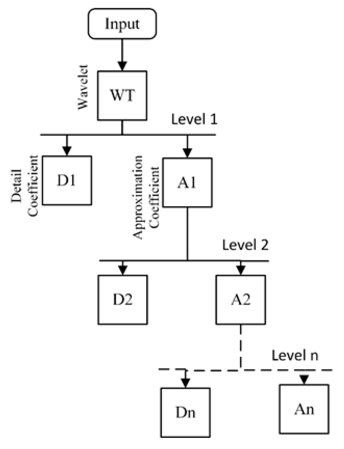
2.1. Wavelet Transform

The electric power load series has some consistent features such as variations in trends, level and slope, and seasonality. These features are often the most important and critical factors that cause load signal instability.
Hence, it is vital to delve extensively into the load series in order to get greater precision. It has been observed that the load series always has diverse frequency components, which are extremely difficult to manage. Wavelets are used to overcome the problem of instability because they produce better compact projections of the signal over time and frequency domains [8]. Furthermore, the wavelet decomposition may be utilized to illustrate primary load pattern characteristics, which are important for greater accurate forecasting. The WT was successfully used for STLF by subdividing the load data into a set of sub-components [22,23,24]. Meanwhile, it can also play a very great role in the prediction process.
In this study, the WT is utilized to classify the load sequence into a combination of multiple sub-components with discrete frequencies [28]. The basic principle of the WT-based decomposition procedure, as shown in Figure 1. The “high-frequency” components giving precise features and abnormal related data about the load demand [29]. Furthermore, these sub-components perform better than the actual load sequence and, as a result, could be approximated rather precisely [30].
According to the literature survey, the WT is classified into two types: “(1) continuous wavelet transform (CWT) and (2) discrete wavelet transform (DWT)”. However, since the CWT examines the mother functions continually and generates a large quantity of data, it is complicated and time consuming to conduct. On the other hand, DWT computes parameters in discrete values, which is substantially faster. As a result, we utilized a DWT in this investigation. Furthermore, wavelet analysis, in general, involves two fundamental functions: the mother wavelet and the scaling functions. The mathematical representation of DWT with the input signal x(t) and mother wavelet function ψ   ( t ) can be expressed by [31]:
D W T   ( m s c ,   k s h ) =   1 a s c . t T x ( t ) . ψ   ( t )
where, m s c ,   k s h are the scale and shift parameters, respectively.
(i)
Scale parameter (   a s c )
  a s c = a 0 m s c  
where, a0 is constant
(ii)
Mother function ( ψ   ( t )   )
ψ   ( t ) = ψ ( k s h b s h a s h )  
where,
(iii)
Shifting parameter ( b s h )
  b s h = n . b 0 . a 0 m s c  
where, n is discrete-time index and b0 is the constant
(iv)
Scaling function ( φ ( m s c , k s h ) ( t ) )
φ ( m s c , k s h ) ( t ) = 2 m s c 2   φ ( 2 m s c ,   t n )  
The detailed ( D m , k c ) and approximation ( A m , k c ) coefficients are
D m , k c = t T x ( t ) .   ψ m , k ( t )  
  A m , k c = t T x ( t ) .   φ m , k ( t )  
The approximation ( A I c ) and detailed ( D J c )   of the signals at the particular scales I and J are calculated by
  A I c = k =   A m , k c   .   φ m , k ( t )  
  D J c = t =   D m , k c   .   ψ m , k ( t )  
As result, the load series ( x ( t ) ) can be represented with mother wavelet   ( ψ ( t ) ) , and its accompanying scaling function ( φ m , k ( t ) ) is expressed as follows:
x ( t ) =   t T A I c ( t ) .   φ m s c , k s h ( t ) +   t T k = D J c . ψ m , k ( t )  
An intuitive sample of two-level decomposition for the load series given by
x ( t ) = A L 1 ( t ) + D L 1 ( t ) = A 21 ( t ) + D 21 ( t ) + D L 1 ( t )      
The load series x ( t ) is decomposed into a set of sub-components:   A L 2 ,   D L 2 ,   a n d   D L 1 . The approximation component A L 2 reflects the general trend and presents a smooth form of x ( t ) . The details terms D 21 ( t )   a n d   D L 1 ( t ) describe the high-frequency components in   x ( t ) .

2.2. Wavelet-Based Ensemble Approach

The mother wavelet and the number of decomposition levels are two critical factors required in the WT. Currently, there is no specific best methodology for selecting such specifications [32]. Numerous studies have been conducted on different wavelet coefficients and appropriate settings have been identified based on the results.
Unfortunately, there are at least three difficulties with this sort of selection approach:
  • Normally, it would take an excessively long amount of time to test a variety of wavelet specifications.
  • The load series may not always be accurately represented by the fixed specification [29].
  • Third, a given set of wavelet coefficients cannot always provide the best predicting outcomes in all perspectives.
To address the aforementioned issues, a wavelet-based ensemble approach is proposed in this paper (as shown in Figure 2). The wavelet transform is used to construct an ensemble of predictors, with each predictor having a distinct combination of mother wavelets and several decomposition levels. A schematic diagram of this type of predictor is shown in Figure 2a,b.
In Figure 2a, the process of estimating the load is as follows: First, the input dataset is divided into two parts, which are time and load. The load is divided into weekday and weekend loads. Then, the load-dependent input is assigned to a particular WT and the resulting output and time-dependent inputs are distributed to another WT to estimate the load. This process continues until the desired best results are achieved by changing the decomposition levels and appropriate parameters in WT.
Similarly, the ensemble forecasting model was constructed by using the model shown in Figure 2b. Here, the models are connected sequentially, one by one, to form a novel WT-based ensemble for predicting the load values. By changing the decomposition levels and appropriate parameters in WT, the desired results can be achieved. The remaining technical details regarding the wavelets and specific parameters used in this study are mentioned clearly as follows:
The wavelet family of “Daubechies (db)” has been frequently utilized to analyze load data in STLF [33,34,35]. Furthermore, it has been observed that “Coiflets (coif)” can also provide a good representation in the results, even though they are rarely used in the literature. Moreover, the mother wavelet order is usually between 2 and 5, and the decomposition levels are less than 4. As a result, eight wavelet functions (“db2-db5 and coif2-coif5”) are employed in this work, with the level of decomposition ranging from 1 to 3. Therefore, the proposed ensemble scheme comprises 24 different wavelet parameter combinations in total.
The mother wavelets of db and coif with particular family numbers are shown in Figure 3. It has been observed that wavelet function changes only in a short period of time. Because the wavelet functions have varied forms, their associated sub-components will behave differently as well. For example, a load signal is divided into three levels that would use the wavelet techniques described above. The resultant approximation aspects are depicted in Figure 4, where Figure 4a corresponds to db and Figure 4b belongs to coif wavelets, respectively.
Furthermore, the wavelet-based ensemble approach will generate distinct input parameters for each forecaster, which could also increase the ensemble’s diversity. Each forecast is updated based on the factors that differ from those used in other factors. As a result, each forecast in the ensemble would contain some unique information regarding the input. The ensemble technique can increase prediction capabilities by utilizing the relevant supplementary information. Furthermore, the ensemble technique will help to select appropriate wavelet parameters and decrease the biases caused by arbitrary wavelet parameters. The results demonstrate that upgrading the model structure and using the ensemble technique may significantly improve forecasting performance.

3. Description of the Input Data

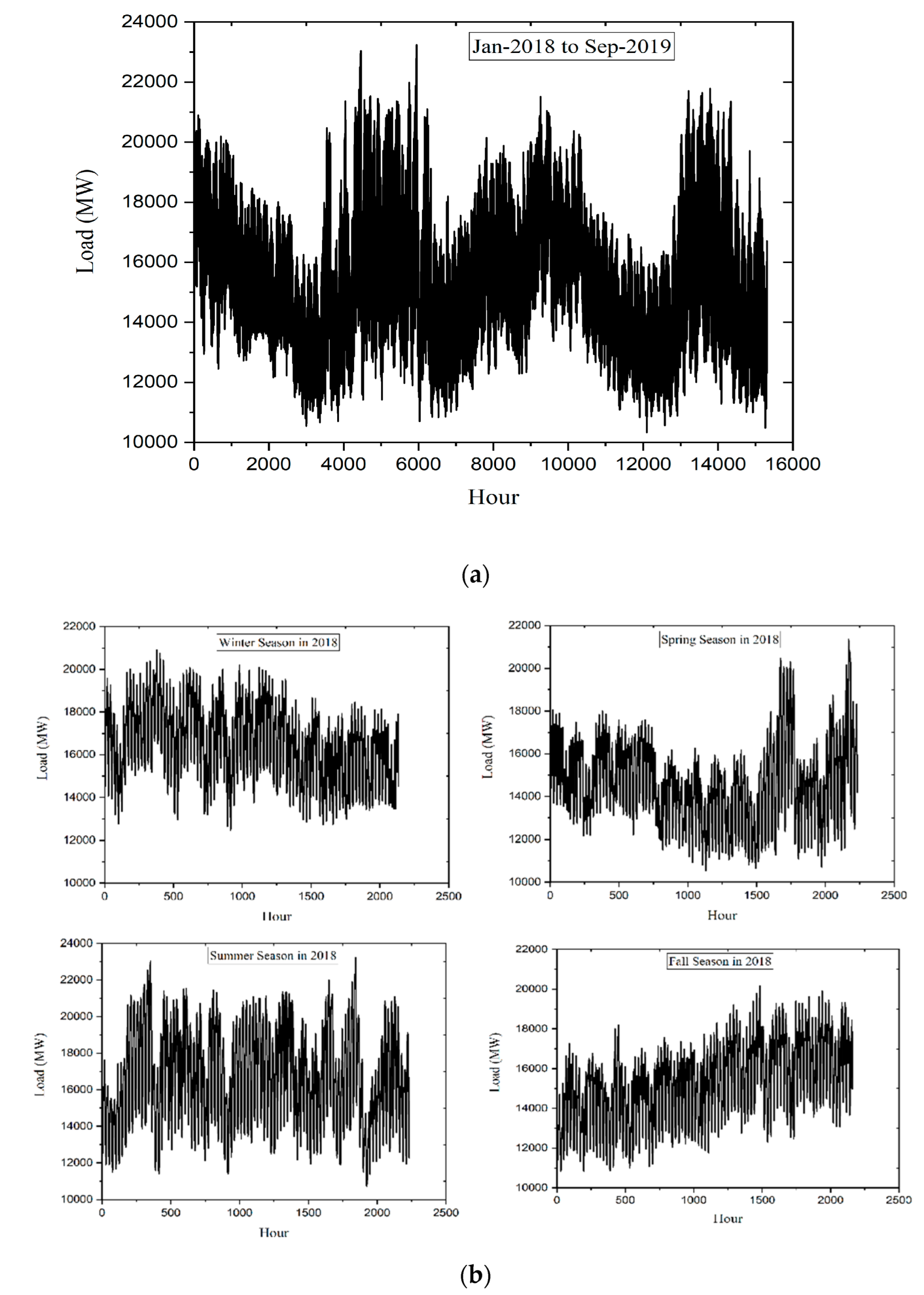
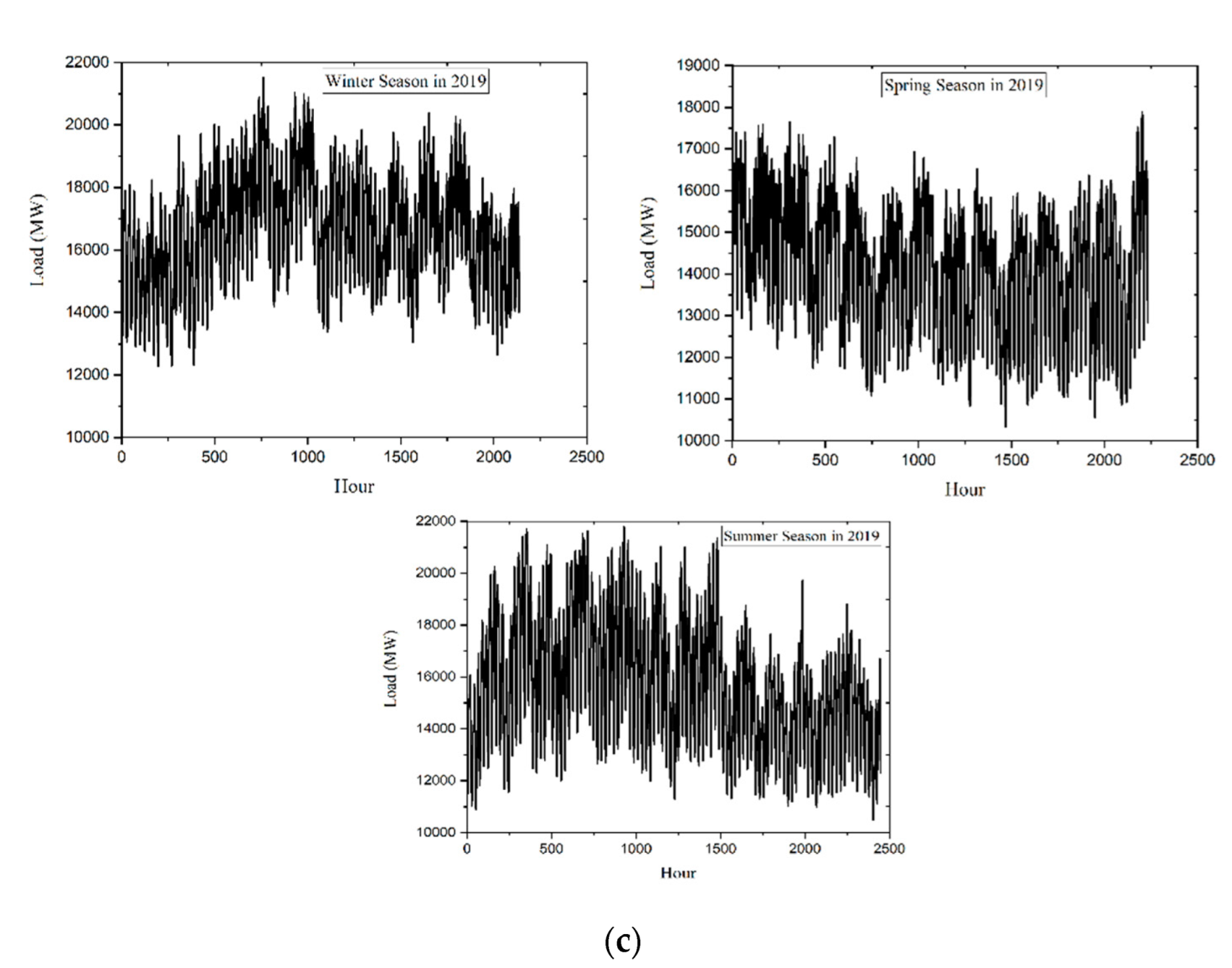
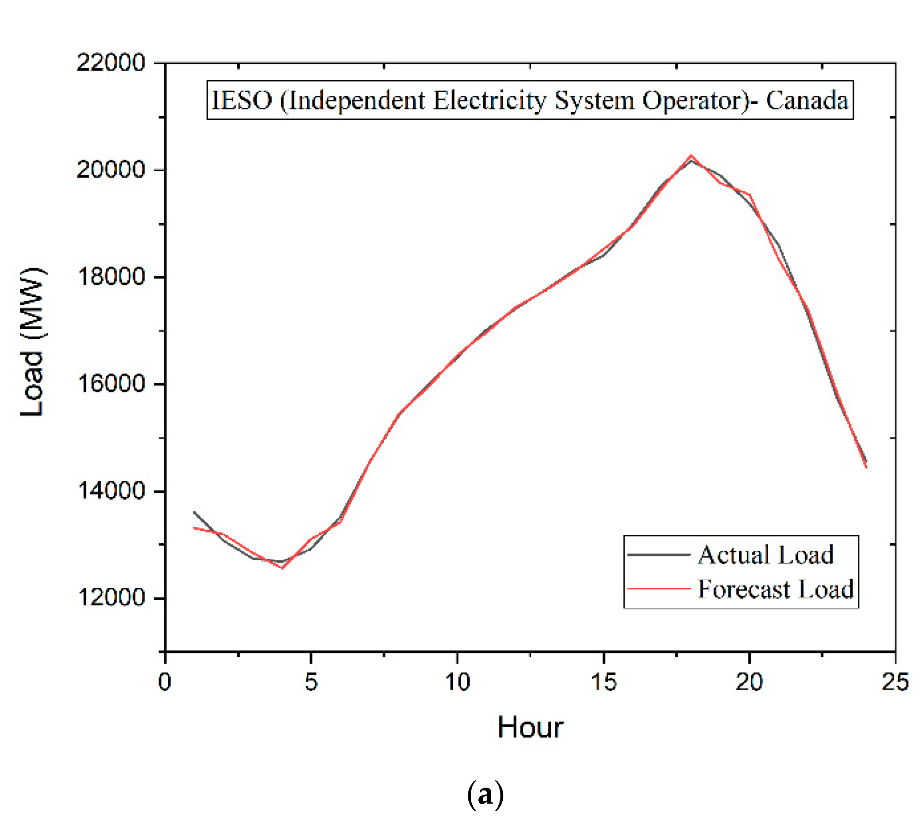
3.1. About the Input Data

In this paper, we have taken the input dataset from the “Ontario (IESO-Canada)” [28], as shown in Figure 5, However, we considered the hourly load series from 1 January 2017 to 30 September 2019 for analysis purposes, as shown in Figure 5a. In addition, the seasonal loads for the years 2018 and 2019 are shown in Figure 5b,c, respectively. The load data shows some non-stationary features, including trends, scale, slope, and seasonality. Hence, the principle aspect of this paper is to forecast the electricity load for the year 2019 by seasonal month and day, considering the daily load demand from the previous year (i.e., 2018). For this purpose, the training and test set data are required to make the model work effectively. Therefore, the different forms of datasets and how they are used in the forecasting process are shown in Table 1, in which the test dataset was considered for model evaluation. This component is useful to see how well the model works in practical applications. Therefore, the last two months in the dataset were selected as the test set required to test the model [20].
Another important thig to note is that factors affecting the load profile, such as temperature, humidity, price, etc., were not considered in this research work, because the “ISEO-Canada” database contains load values that are recorded based on the geographical and seasonal weather conditions. In addition, many studies have demonstrated appropriate correlational solutions for selecting input features. They concluded that power consumption depends on seasonal weather conditions, relative time, and geographical location [35,36,37,38,39,40,41,42]. Therefore, only power load values are considered here based on seasonality with respect to time.

3.2. Statistical Summary Analysis of Input Data

The hourly power consumption data from 1 January 2018 to 30 September 2019, from the Ontario grid, are taken as the input data, in which there are approximately 15,312 values in the total input data at a rate of 24 values per day, for each day of each month. A summary of input data per hour is as follows: The total load value was 23,895,0219 MW, the average value was 1,560,583 MW, and the minimum and maximum values were 10,328 MW and 23,240 MW, respectively; in addition, the total data range value was 12,912 MW. Similarly, Table 2 shows the complete summary analysis of the training and testing set data, respectively.
The table contains the following information. For the summer period, the load distribution value was 1,447,989,720 MW, which is 61% of the overall input. This means that electricity consumption was very high in this season. This may be due to rising temperatures caused by changes in the climate. Similarly, the load value during the fall season was 137,436,546 MW, which is 56% of the total load. This means that power consumption was very low due to the declining temperatures in this season.
However, when it comes to average values, the load value (15,769.39189 MW) during the spring season had a higher value than the total load average value (15,605.42183 MW). In addition, the fall season had the lowest average value (15,465.8903 MW). When it comes to minimum and maximum load values, the winter, spring, summer, and fall seasons had the same values. Furthermore, the maximum value is recorded during the fall season (21,791 MW). The winter and spring seasons had a unique range value (12,699 MW). Moreover, the summer and fall seasons had values of 12,912 MW and 11,463 MW, respectively. Similarly, during the fall season, the highest load value was recorded (22,143,585 MW), which is 93% of the total load. In addition, summer had the lowest value (20,585,179 MW), which is 86% of the total load.
From the above discussion, we can conclude that the electricity consumption mostly depends on seasonal weather conditions. Hence, only previous load values with time factors are considered in this paper.

4. Results and Discussion
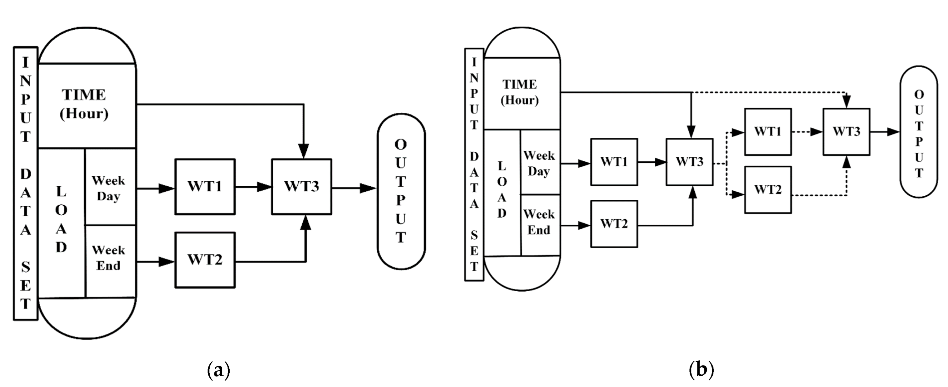
The forecasting of load with limited historical data may provide insufficient information. Therefore, several comprehensive methods have been proposed in the past to overcome this problem. In this order, an ensemble approach has been developed in this paper to improve LF performance further. The suggested model has been validated using a real-world electrical dataset, and its performance has been compared with other state-of-the-art methods using three error metrics, which are: “mean absolute percentage error (MAPE), mean absolute error (MAE), and root mean square error (RMSE)”. They are defined as follows:
M A P E = 1 n   i = 1 n | L a c t u a l L f o r e c a s t e d ^ L a c t u a l | 100  
M A E = 1 n   i = 1 n | L a c t u a l L f o r e c a s t e d ^ |  
R M S E = 1 n i = 1 n ( L a c t u a l L f o r e c a s t e d ^ ) 2      
Here, n represents the total no of input values, L a c t u a l   denotes the real or actual load, and L f o r e c a t e d ^   denotes the predicted load value.
This research was carried out by setting up the model proposed in this paper based on the MATLAB software on a personal Acer laptop, which has Intel (R), i5, 2.60, 4 GHz, 4 GB RAM and a 64-bit processor. The results and performance details of the model in various case studies are as follows:
(1).
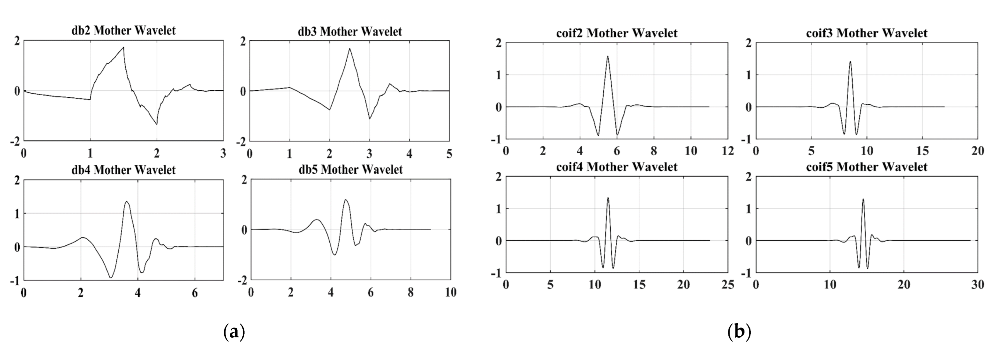
Model-1 (M1): db wavelets were used in three blocks. The arrangement of this model is shown in Figure 2a.
(2).
Model-2 (M2): In this case, the model M1 blocks were replaced with coif wavelets.
(3).
Model-3 (M3): The proposed model was tested in 4 optimum ways from all the possible combinations with db and coif, resulting in the appropriate model (M3).
(4).
Model-4 (M4): Based on Model M3, we developed an ensemble wavelet-based model, as shown in Figure 2b.
The results achieved by providing the appropriate input data to the above models in various case studies are described in the next section.

4.1. Case Studies Analysis

The model proposed in this paper was tested in four different cases, and these models have shown interesting results in each case. These are as follows:
Case (I): In this case, the db wavelet was used in the model M1 to estimate the load. The detailed results are given in Table 3 and Table 4. Table 3 contains load estimation error values for different seasons by either weekday or weekend, while Table 4 shows errors for different seasons by month.
From the results obtained by this model, it was observed that the winter weekend had the lowest MAPE (1.353%) and the spring weekend had the lowest MAE (174 MW). Similarly, when it comes to high values, the spring and summer weekends had a MAPE of 1.9111% and MAE of 669 MW. Furthermore, with respect to the monthly (Table 4) forecast errors during different seasons, the minimum MAPE value in the winter was 1.4758%, and MAE was 80 MW in the fall season. On the other hand, in terms of higher values, the fall season had a MAPE value of 1.7375%, and in the winter season, MAE was 94 MW.
From the above results, the proposed model works well in terms of load estimation. Furthermore, these results show a reduction in the error when compared to WT-based ANN [28].
Case (II): In this case, the coif wavelet was used to estimate the load with the model M2. The results obtained when testing the model through input data can be seen in Table 3 and Table 4. From the results, it was observed that the spring weekend had the lowest MAPE (1.2445%) value, while the winter weekday had the lowest MAE (171 MW). Similarly, when it comes to high values, the fall weekday had a MAPE of 1.9801% and the summer weekday had a MAE of 506 MW. Furthermore, when it comes to the seasonal (Table 4) forecast errors during different seasons, the minimum MAPE value in the winter was 1.2162%, and MAE was 51 MW in the fall season. On the other hand, in terms of higher values, the MAPE value was 1.9320% during the fall season and MAE was 70 MW in the winter season.
Case (III): As mentioned previously, the M3 model is a combination of two wavelets (i.e., db and coif). The proposed model showed expected results when validated with a training and testing set, with an input dataset. These results are shown in Table 3 and Table 4. The details of the estimated results of electricity consumption with the M3 model are as follows: It was observed that the fall weekday had the lowest MAPE (1.1153%) value, while the winter weekend had the lowest MAE (132 MW). Similarly, when it comes to high values, the summer weekend had a MAPE of 1.8321% and the summer weekday had a MAE of 488 MW. Furthermore, in terms of the month-wise (Table 4) forecast errors during the different seasons, the minimum MAPE value in the fall season was 1.3552%, and MAE was 72 MW. On the other hand, in terms of higher values, the MAPE value was 1.7150% and MAE was 107 MW during the summer season. When comparing the findings of the proposed model with the WT-based ANN approach, these results seem promising.
Case (IV): The order in which the models are constructed was one after the other, to form a wavelet-based ensemble model, as shown in Figure 2b. For this purpose, the structure of the M3 model which used the same as the optimum model 3. In this research, we have considered it as a proposed model (M4). The forecasted results are listed in the tables. From the results obtained by this model, it was observed that the spring weekday had the lowest MAPE (0.1521%) value, while the winter weekend had the lowest MAE (91 MW). Similarly, when it comes to high values, the spring weekend had a MAPE of 0.5183% and the fall weekday had a MAE of 424 MW. Furthermore, when it comes to the monthly (Table 4) forecast errors during different seasons, the minimum MAPE value in the summer was 0.5914%, and MAE was 51 MW in the fall season. On the other hand, in terms of higher values, the MAPE value was 0.6777% and MAE was 62 MW during the spring season. It is clear that these results are more accurate than other WT-based ANN methods.
The summary of the results of this proposed model is as follows:
  • The errors in the results when estimating all-season loads using the model M1 are as follows: First, the summer season weekday (1.1576%) had the lowest error. Second, there was an error of 1.1353% and 1.4758% during the winter weekends and seasons, respectively.
  • When estimating all-season loads with the help of model M2, the spring season had error values of 1.2445% and 1.3641%, respectively. However, in winter, the error value was 1.2163%.
  • The model M3 had an error value of 1.1153% and 1.2379%, respectively, during the summer season weekdays, and 1.3532% during the months of fall.
  • Based on the productivity results of the suggested model (M4), the spring weekday had an error of 0.1521%, and the weekend had an error of 0.2482%.

4.2. Validation of the Proposed Model with Various Datasets
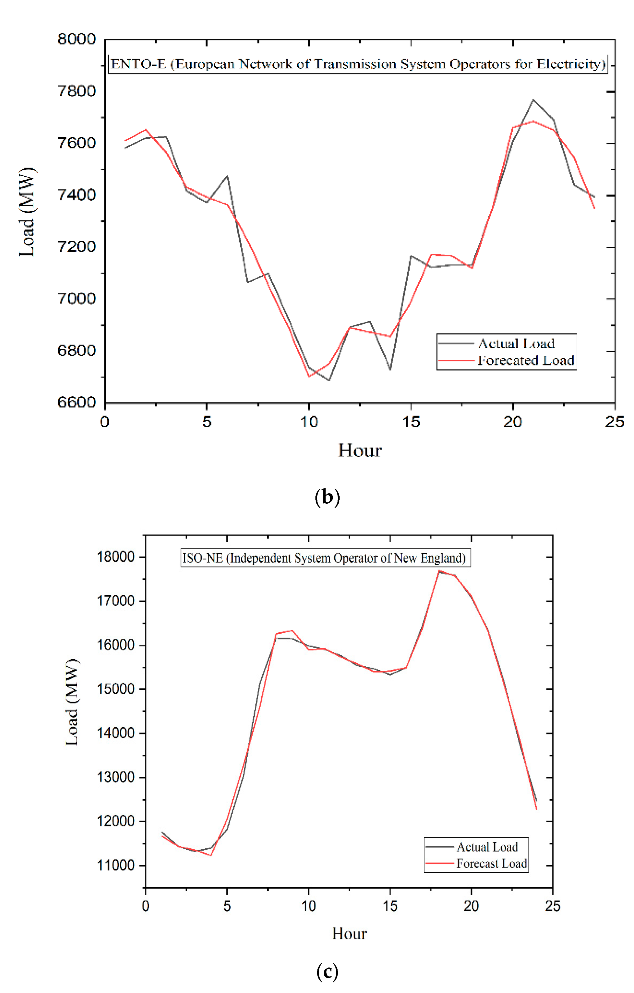
This section describes the performance and validation details of the proposed model based on errors such as MAPE, MAE, and RMSE, with the public datasets, IESO-Canada, ISO-NE, and ENTSO-E, were taken as the input to the proposed model. In addition, the comparative analysis of the model with different models are presented and the results are as follows:

4.2.1. IESO-Canada

In this analysis, IESO-Canada data from 2014–15 were used as the input for the proposed model. Based on this data, the load was estimated for the month and day of the year 2016. The forecasted results of the proposed model in terms of MAPE are given in Table 5. Furthermore, the proposed model appears to have a better forecast performance than another existing model. The average accuracy of the proposed model for the monthly forecasted load is 98.56%, while the model in [28] is 98.34%. Therefore, our model works 22% more effectively than other models and exhibits accuracy. However, when it comes to the weekend vs. weekday values, the accuracy of the model is 99.02%, and the other model is 98.82%. This means that the performance of the suggested model is 20% more effective. Hence, the proposed model appears to have a better forecast performance than another model.

4.2.2. ENTSO-E

The performance of the proposed model in this analysis was tested with the ENTO-E dataset. According to the authors in [43], the same data segmentation (such as “training and testing”) was considered for this validation. The model results are compared with the models proposed in [43,44,45], respectively. Finally, the forecasted load values of the model, with help from all three errors, are listed in Table 6.
From the literature [43], it is understood that the error value (% MAPE) for the ENTSO European grid is more because the model cannot understand data that have a slightly different distribution with training and testing. The model undergoing testing was also highly affected by the quality of the ENTSO-European dataset.
Furthermore, the proposed model appears to have a better forecast performance than another existing model. The accuracy of the proposed model in forecasting load is 98.03%, while the model in [44] is 97.55%. Therefore, the suggested model works 48% more effectively than the other model and exhibits accuracy. However, when it comes to [45], the accuracy of the model is 97.78%. This means that the performance of the suggested model is 25% more effective than the rest. Similarly, the accuracy of the model in [43] is 97.76%. Therefore, the proposed model works 27% more effectively than the other model. Finally, when it comes to [43], the accuracy of the model is 97.98%. This means that the performance of the suggested model is 5% more effective than the rest. When it comes to the values of the other errors (MAE and RMSE), the performance of the proposed model has improved as expected. Hence, the proposed model appears to have a better forecast performance than other models.

4.2.3. ISO-NE

Here, the input data from 1 March 2003 to 31 December 2014 were taken from the ISO-NE database to test the generalization capability of the proposed model in two ways [46]. However, estimating the daily loads for 2006 on the dataset was considered the first test case. Subsequent examination of model capability on the 2010 and 2011 data is considered a second case. The load forecasted details regarding test cases and comparative analysis with respective models are as follows:

Test Case 1

In this test case, the proposed model performance was validated or examined to predict the load in 2006. The period of data from 1 June 2003 to 31 December 2005 was utilized for the model. The results are compared with the models proposed in [33,36,37,38], respectively. The forecasted results, in the form of error matrices, are tabulated in Table 7.
The proposed model with the lowest total MAPE can be seen in the table. While this is the case, the WT-ELM-MABC [47] and ResNetPulse [46] models also show good results. The accuracy of the proposed model in terms of the forecasted load is 98.76%, while the model in [31] is 98.27% accurate. Therefore, our model works 49% more effectively than the other model and exhibits accuracy. However, when it comes to [21], the accuracy of the model is 98.511%, meaning that the performance of the suggested model is 25% more effective than the rest. Similarly, the model in [47] is 98.52%. Therefore, the proposed model works 24% more effectively than the other model. Finally, when it comes to [46], the accuracy of the model is 98.55%, meaning that the performance of the suggested model is 20% more effective than the rest. Therefore, when testing the proposed model with different datasets, it becomes clear that it has the expected results and normalization capability.

Test Case 2

In this case, the proposed model capability was investigated by estimating the load for the years 2010 and 2011, respectively. The data were used to train the model from 1 January 2004 to 31 December 2009. The performance of the suggested model comparative results with other models are tabulated in Table 8. Results show that the proposed model outperforms the prevailing models concerning the total MAPE for the two years, and an enhancement of 25% and 41% is attained for the years 2010 and 2011, respectively.
Therefore, the proposed model shows excellent performance when compared with other models. This suggests that the proposed model works well for the respective datasets. In addition, this wavelet-based ensemble model provides insight into sequence data. The ensemble structure facilitates model self-correction by associating the output of the first model with recent or short-sequence data. In addition, it can be understood that the proposed method is performing better than other reference models. Therefore, the %MAPE of the proposed method is displayed in the last row of Table 7 and Table 8 by comparing with other existing models available in the literature. In addition, Figure 6 illustrates the 24-h load estimation results of the proposed model for the various public datasets.

5. Conclusions

This paper proposes a unique ensemble of the wavelet-based model to improve STLF accuracy. An ensemble of db and coif wavelets is used to develop the model. This STLF technique is evaluated with data from the Ontario, Canada, power market, and errors such as MAPE, MAE and RMSE are calculated. According to the observations, the proposed technique has the lowest prediction error (MAPE) on weekdays and weekends, at 0.96% and 1.01%, respectively. Furthermore, the performance of the model is validated with the datasets available in the literature. From the results, the proposed model for forecasting will give minimal error. The comparison results (including forecast curve, prediction error, and accuracy) demonstrate that the proposed approach has great potential to forecast real-time electricity demand. Further this novel method may be extended for generation dispatch and price forecasting in the micro grid/smart grid environment.

Author Contributions

Conceptualization, V.Y.K. and B.S.; methodology, V.Y.K.; software, V.Y.K.; validation, V.Y.K., B.S.; formal analysis, B.S.; investigation, V.Y.K. and B.S.; resources, V.Y.K. and B.S.; data curation, V.Y.K.; writing—original draft preparation, V.Y.K.; writing—review and editing, B.S.; visualization, V.Y.K.; supervision, B.S.; project administration, B.S.; funding acquisition, Not applicable. All authors have read and agreed to the published version of the manuscript.

Funding

This research received no external funding.

Institutional Review Board Statement

Not applicable.

Informed Consent Statement

Not applicable.

Data Availability Statement

Not applicable.

Conflicts of Interest

The authors declare no conflict of interest.

References

  1. Young, P.C. Book Review: Comparative Models for Electrical Load Forecasting. IEE Proc. D Control Theory Appl. 1986, 133, 143. [Google Scholar] [CrossRef]
  2. Raza, M.Q.; Khosravi, A. A Review on Artificial Intelligence Based Load Demand Forecasting Techniques for Smart Grid and Buildings. Renew. Sustain. Energy Rev. 2015, 50, 1352–1372. [Google Scholar] [CrossRef]
  3. Cheepati, K.R.; Nageswara Prasad, T. Performance Comparison of Short Term Load Forecasting Techniques. Int. J. Grid Distrib. Comput. 2016, 9, 287–302. [Google Scholar] [CrossRef]
  4. Kondaiah, V.Y.; Saravanan, B.; Sanjeevikumar, P.; Khan, B. Review on Short-term Load Forecasting Models for Micro-grid Application. J. Eng. 2022, 2022, 665–689. [Google Scholar] [CrossRef]
  5. Paparoditis, E.; Sapatinas, T. Short-Term Load Forecasting: The Similar Shape Functional Time-Series Predictor. IEEE Trans. Power Syst. 2013, 28, 3818–3825. [Google Scholar] [CrossRef] [Green Version]
  6. Dodamani, S.N.; Shetty, V.J.; Magadum, R.B. Short Term Load Forecast Based on Time Series Analysis: A Case Study. In Proceedings of the IEEE International Conference on Technological Advancements in Power and Energy, TAP Energy, Kollam, India, 24–26 June 2015. [Google Scholar]
  7. Haq, M.R.; Ni, Z. A New Hybrid Model for Short-Term Electricity Load Forecasting. IEEE Access 2019, 7, 125413–125423. [Google Scholar] [CrossRef]
  8. Dhaval, B.; Deshpande, A. Short-Term Load Forecasting with Using Multiple Linear Regression. Int. J. Electr. Comput. Eng. 2020, 10, 3911–3917. [Google Scholar] [CrossRef]
  9. Li, C.; Chiang, T.W. Complex Neurofuzzy ARIMA Forecasting—A New Approach Using Complex Fuzzy Sets. IEEE Trans. Fuzzy Syst. 2013, 21, 567–584. [Google Scholar] [CrossRef]
  10. Lopez, J.C.; Rider, M.J.; Wu, Q. Parsimonious Short-Term Load Forecasting for Optimal Operation Planning of Electrical Distribution Systems. IEEE Trans. Power Syst. 2019, 34, 1427–1437. [Google Scholar] [CrossRef] [Green Version]
  11. Zheng, J.; Huang, M. Traffic Flow Forecast through Time Series Analysis Based on Deep Learning. IEEE Access 2020, 8, 82562–82570. [Google Scholar] [CrossRef]
  12. Rocha, L.G.; Goias, E.D.; Alcala, S.G.S.; Garces Negrete, L.P. Short-Term Electric Load Forecasting Using Neural Networks: A Comparative Study. In Proceedings of the 2020 IEEE PES Transmission and Distribution Conference and Exhibition—Latin America, Montevideo, Uruguay, 28 September–2 October 2020. [Google Scholar]
  13. Dagdougui, H.; Bagheri, F.; Le, H.; Dessaint, L. Neural Network Model for Short-Term and Very-Short-Term Load Forecasting in District Buildings. Energy Build. 2019, 203, 109408. [Google Scholar] [CrossRef]
  14. Drgoňa, J.; Arroyo, J.; Cupeiro Figueroa, I.; Blum, D.; Arendt, K.; Kim, D.; Ollé, E.P.; Oravec, J.; Wetter, M.; Vrabie, D.L.; et al. All You Need to Know about Model Predictive Control for Buildings. Annu. Rev. Control 2020, 50, 190–232. [Google Scholar] [CrossRef]
  15. Khosravi, A.; Nahavandi, S. Load Forecasting Using Interval Type-2 Fuzzy Logic Systems: Optimal Type Reduction. IEEE Trans. Ind. Inform. 2014, 10, 1055–1063. [Google Scholar] [CrossRef]
  16. Wu, J.; Cui, Z.; Chen, Y.; Kong, D.; Wang, Y.G. A New Hybrid Model to Predict the Electrical Load in Five States of Australia. Energy 2019, 166, 598–609. [Google Scholar] [CrossRef]
  17. Cecati, C.; Kolbusz, J.; Rózycki, P.; Siano, P.; Wilamowski, B.M. A Novel RBF Training Algorithm for Short-Term Electric Load Forecasting and Comparative Studies. IEEE Trans. Ind. Electron. 2015, 62, 6519–6529. [Google Scholar] [CrossRef]
  18. Kalakova, A.; Kumar Nunna, H.S.V.S.; Jamwal, P.K.; Doolla, S. A Novel Genetic Algorithm Based Dynamic Economic Dispatch with Short-Term Load Forecasting. IEEE Trans. Ind. Appl. 2021, 57, 2972–2982. [Google Scholar] [CrossRef]
  19. Liao, Z.; Pan, H.; Fan, X.; Zhang, Y.; Kuang, L. Multiple Wavelet Convolutional Neural Network for Short-Term Load Forecasting. IEEE Internet Things J. 2021, 8, 9730–9739. [Google Scholar] [CrossRef]
  20. Liu, Y.; Dutta, S.; Kong, A.W.K.; Yeo, C.K. An Image Inpainting Approach to Short-Term Load Forecasting. IEEE Trans. Power Syst. 2022, in press. [Google Scholar] [CrossRef]
  21. Li, S.; Goel, L.; Wang, P. An Ensemble Approach for Short-Term Load Forecasting by Extreme Learning Machine. Appl. Energy 2016, 170, 22–29. [Google Scholar] [CrossRef]
  22. Li, Y.; Zhang, H.; Liang, X.; Huang, B. Event-Triggered-Based Distributed Cooperative Energy Management for Multienergy Systems. IEEE Trans. Ind. Inform. 2019, 15, 2008–2022. [Google Scholar] [CrossRef]
  23. Liu, Z.; Li, W.; Sun, W. A Novel Method of Short-Term Load Forecasting Based on Multiwavelet Transform and Multiple Neural Networks. Neural Comput. Appl. 2013, 22, 271–277. [Google Scholar] [CrossRef]
  24. Tayab, U.B.; Zia, A.; Yang, F.; Lu, J.; Kashif, M. Short-Term Load Forecasting for Microgrid Energy Management System Using Hybrid HHO-FNN Model with Best-Basis Stationary Wavelet Packet Transform. Energy 2020, 203, 117857. [Google Scholar] [CrossRef]
  25. Moradzadeh, A.; Zakeri, S.; Shoaran, M.; Mohammadi-Ivatloo, B.; Mohammadi, F. Short-Term Load Forecasting of Microgrid via Hybrid Support Vector Regression and Long Short-Term Memory Algorithms. Sustainability 2020, 12, 7076. [Google Scholar] [CrossRef]
  26. Aly, H.H.H. A Proposed Intelligent Short-Term Load Forecasting Hybrid Models of ANN, WNN and KF Based on Clustering Techniques for Smart Grid. Electr. Power Syst. Res. 2020, 182, 106191. [Google Scholar] [CrossRef]
  27. Li, H.; Phung, D. An Introduction to Variable and Feature Selection. J. Mach. Learn. Res. 2014, 3, 1157–1182. [Google Scholar]
  28. Daubechies, I. Ten Lectures on Wavelets. Math. Comput. 1993, 61, 941–942. [Google Scholar] [CrossRef]
  29. Anbazhagan, S.; Vaidehi, K. Short-Term Load Forecasting Using Wavelet De-Noising Signal Processing Techniques. In Data Engineering and Communication Technology; Advances in Intelligent Systems and Computing; Springer: Singapore, 2020. [Google Scholar]
  30. Bento, P.M.R.; Pombo, J.A.N.; Calado, M.R.A.; Mariano, S.J.P.S. Optimization of Neural Network with Wavelet Transform and Improved Data Selection Using Bat Algorithm for Short-Term Load Forecasting. Neurocomputing 2019, 358, 53–71. [Google Scholar] [CrossRef]
  31. El-Hendawi, M.; Wang, Z. An Ensemble Method of Full Wavelet Packet Transform and Neural Network for Short Term Electrical Load Forecasting. Electr. Power Syst. Res. 2020, 182, 106265. [Google Scholar] [CrossRef]
  32. Li, S.; Wang, P.; Goel, L. A Novel Wavelet-Based Ensemble Method for Short-Term Load Forecasting with Hybrid Neural Networks and Feature Selection. IEEE Trans. Power Syst. 2016, 31, 1788–1798. [Google Scholar] [CrossRef]
  33. Bessec, M.; Fouquau, J. Short-Run Electricity Load Forecasting with Combinations of Stationary Wavelet Transforms. Eur. J. Oper. Res. 2018, 264, 149–164. [Google Scholar] [CrossRef]
  34. Chen, Y.; Luh, P.B.; Guan, C.; Zhao, Y.; Michel, L.D.; Coolbeth, M.A.; Friedland, P.B.; Rourke, S.J. Short-Term Load Forecasting: Similar Day-Based Wavelet Neural Networks. IEEE Trans. Power Syst. 2010, 25, 322–330. [Google Scholar] [CrossRef]
  35. Ofori-Ntow, E., Jr.; Ziggah, Y.Y.; Relvas, S. Hybrid Ensemble Intelligent Model Based on Wavelet Transform, Swarm Intelligence and Artificial Neural Network for Electricity Demand Forecasting. Sustain. Cities Soc. 2021, 66, 102679. [Google Scholar] [CrossRef]
  36. Zhang, G.; Guo, J. A Novel Method for Hourly Electricity Demand Forecasting. IEEE Trans. Power Syst. 2020, 35, 1351–1363. [Google Scholar] [CrossRef]
  37. Suryanarayana, G.; Lago, J.; Geysen, D.; Aleksiejuk, P.; Johansson, C. Thermal Load Forecasting in District Heating Networks Using Deep Learning and Advanced Feature Selection Methods. Energy 2018, 157, 141–149. [Google Scholar] [CrossRef]
  38. Dai, Y.; Zhao, P. A Hybrid Load Forecasting Model Based on Support Vector Machine with Intelligent Methods for Feature Selection and Parameter Optimization. Appl. Energy 2020, 279, 115332. [Google Scholar] [CrossRef]
  39. Rafati, A.; Joorabian, M.; Mashhour, E. An Efficient Hour-Ahead Electrical Load Forecasting Method Based on Innovative Features. Energy 2020, 201, 117511. [Google Scholar] [CrossRef]
  40. Valente, J.M.; Maldonado, S. SVR-FFS: A Novel Forward Feature Selection Approach for High-Frequency Time Series Forecasting Using Support Vector Regression. Expert Syst. Appl. 2020, 160, 113729. [Google Scholar] [CrossRef]
  41. Lahouar, A.; Ben Hadj Slama, J. Day-Ahead Load Forecast Using Random Forest and Expert Input Selection. Energy Convers. Manag. 2015, 103, 1040–1051. [Google Scholar] [CrossRef]
  42. Pramono, S.H.; Rohmatillah, M.; Maulana, E.; Hasanah, R.N.; Hario, F. Deep Learning-Based Short-Term Load Forecasting for Supporting Demand Response Program in Hybrid Energy System. Energies 2019, 12, 3359. [Google Scholar] [CrossRef] [Green Version]
  43. Tian, C.; Ma, J.; Zhang, C.; Zhan, P. A Deep Neural Network Model for Short-Term Load Forecast Based on Long Short-Term Memory Network and Convolutional Neural Network. Energies 2018, 11, 3493. [Google Scholar] [CrossRef] [Green Version]
  44. Kong, W.; Dong, Z.Y.; Jia, Y.; Hill, D.J.; Xu, Y.; Zhang, Y. Short-Term Residential Load Forecasting Based on LSTM Recurrent Neural Network. IEEE Trans. Smart Grid 2019, 10, 841–851. [Google Scholar] [CrossRef]
  45. Chen, K.; Chen, K.; Wang, Q.; He, Z.; Hu, J.; He, J. Short-Term Load Forecasting with Deep Residual Networks. IEEE Trans. Smart Grid 2019, 10, 3943–3952. [Google Scholar] [CrossRef] [Green Version]
  46. Li, S.; Wang, P.; Goel, L. Short-Term Load Forecasting by Wavelet Transform and Evolutionary Extreme Learning Machine. Electr. Power Syst. Res. 2015, 122, 96–103. [Google Scholar] [CrossRef]
  47. Yu, H.; Reiner, P.D.; Xie, T.; Bartczak, T.; Wilamowski, B.M. An Incremental Design of Radial Basis Function Networks. IEEE Trans. Neural Netw. Learn. Syst. 2014, 25, 1793–1803. [Google Scholar] [CrossRef] [PubMed]
Figure 1. Level-wise decomposition with wavelet transform.
Energies 15 05299 g001
Figure 2. Proposed wavelet-based ensemble model: (a) Proposed wavelet diagram for Model 1, 2, and 3; (b) Proposed wavelet diagram for model 4 (M4).
Energies 15 05299 g002
Figure 3. Mother wavelets at different levels: (a) Four mother wavelets of db family; (b) Four mother wavelets of coif family.
Energies 15 05299 g003
Figure 4. Wavelet approximation coefficients at different levels: (a) db family approximation coefficients; (b) coif family approximation coefficients.
Energies 15 05299 g004
Figure 5. Input load series from 1 January 2018 to 30 September 2019 (IESO-Canada) (a) Input load data from IESO-Canada database; (b) Seasonal input data during the year 2018; (c) Seasonal input data during the year 2019.
Energies 15 05299 g005aEnergies 15 05299 g005b
Figure 6. Forecast results of proposed model with three datasets: (a) IESO-Canada-Dataset; (b) ENTO-European-Dataset; (c) ISO-NE-Dataset.
Energies 15 05299 g006aEnergies 15 05299 g006b
Table 1. Different forms of the input dataset.
Input DataSeasonOutput
(To Forecast Month)
Training SetTesting Set
(Last Two Months from Input Data)
IESO Dataset
1 January 2017
To
30 September 2019
WinterJanuary 2019January 17 to October 18November 18 to December 18
SpringApril 2019April 17 to January 19February 19 to March 19
SummerJuly 2019July 17 to April 19May 19 to June 19
FallOctober 2019October 17 to July 19August 19 to September 19
Table 2. Statistical summary analysis of training and testing datasets.
Statistical Summary Analysis
SeasonTraining Set
Mean (MW)Minimum (MW)Maximum (MW)Range (MW)Sum (MW)Count (Hour)
Winter15,689.1034210,54123,24012,699137,436,5468760
Spring15,769.3918910,54123,24012,699138,139,8738760
Summer15,610.7299610,32823,24012,912147,989,7209480
Fall15,465.8903010,32821,79111,463135,481,1998760
Testing Set
Winter15,881.2711,76520,152838723,250,1781464
Spring16,207.9312,21020,500829022,950,4221416
Summer14,060.9110,32820,248992020,585,1791464
Fall15,125.4010,47721,35410,87722,143,5851464
Table 3. Weekday and weekend seasonal forecasted results.
ModelDayWinter SeasonSpring SeasonSummer SeasonFall Season
MAPE (%)MAE (MW)RMSE (MW)MAPE (%)MAE (MW)RMSE (MW)MAPE (%)MAE (MW)RMSE (MW)MAPE (%)MAE (MW)RMSE (MW)
M1Weekday1.34052473531.65862002861.15766699141.6022486660
Weekend1.13532924181.91111742481.45615327271.2843603823
M2Weekday1.69521712371.24452673231.53135066251.9801343483
Weekend1.52111902641.36412432941.90074075031.6412413583
M3Weekday1.47671562181.65861391821.38694885401.1153482672
Weekend1.55611321831.72451341761.83213704081.2379435605
M4Weekday0.18711111290.15211131220.34323423800.4274424551
Weekend0.4274911090.5183931020.24823213530.2503404521
Table 4. Seasonal forecasted results.
ModelWinter SeasonSpring SeasonSummer SeasonFall Season
MAPE (%)MAE (MW)RMSE (MW)MAPE (%)MAE (MW)RMSE (MW)MAPE (%)MAE (MW)RMSE (MW)MAPE (%)MAE (MW)RMSE (MW)
M11.4758943211.5697883011.6137862941.737580608
M21.2163703311.3086652461.9320562081.621151590
M31.5328722101.3831792191.71501071871.353280553
M40.6145551300.6704621690.5914511390.677760427
Table 5. MAPEs of the proposed model with the IESO-Canada dataset.
MAPE (%) of the Proposed Method with IESO-Dataset
MonthWT based NN [28]Proposed Model
January1.5041.354
February1.6181.266
March1.8881.339
April1.7631.634
May1.4061.354
June1.9611.799
July1.6381.323
August1.6271.512
September1.5081.236
October1.4341.273
November1.7571.554
December2.0241.692
Day(s)
Weekday1.030.96
Weekend1.331.01
Table 6. MAPEs of the proposed model with the ENSTO-E dataset.
ModelMAPE (%)MAE (MW)RMSE (MW)
CNN-LSTM [44]2.45171.71240.57
RNN-LSTM [45]2.22155.83222.44
Waavenet [43]2.24157.28217.98
CNN-LSTM [43]2.02142.23203.23
Proposed1.97127.18188.48
Table 7. MAPEs of the proposed model with the ISO-NE dataset in Test Case 1.
ModelMAPE (%)
SIWNN [34]1.73
WT-ELM-PLSR [21]1.489
WT-ELM-MABC [47]1.48
ResNetPluse [46]1.447
Proposed1.242
Table 8. MAPEs of the proposed model with the ISO-NE dataset in Test Case 2.
ModelMAPE (%)
20102011
RBFN-ErrCorr orginal [44] 1.802.02
RBFN-ErrCorr modified [17]1.751.98
WT-ELM-PLSR [21]1.501.80
ResNetPluse [46]1.501.64
Proposed1.391.45
Publisher’s Note: MDPI stays neutral with regard to jurisdictional claims in published maps and institutional affiliations.

