
Optimizing the Design of a Biomass-to-Biofuel Supply Chain Network Using a Decentralized Processing Approach


Abstract
:1. Introduction
2. Literature Review
3. Methodology
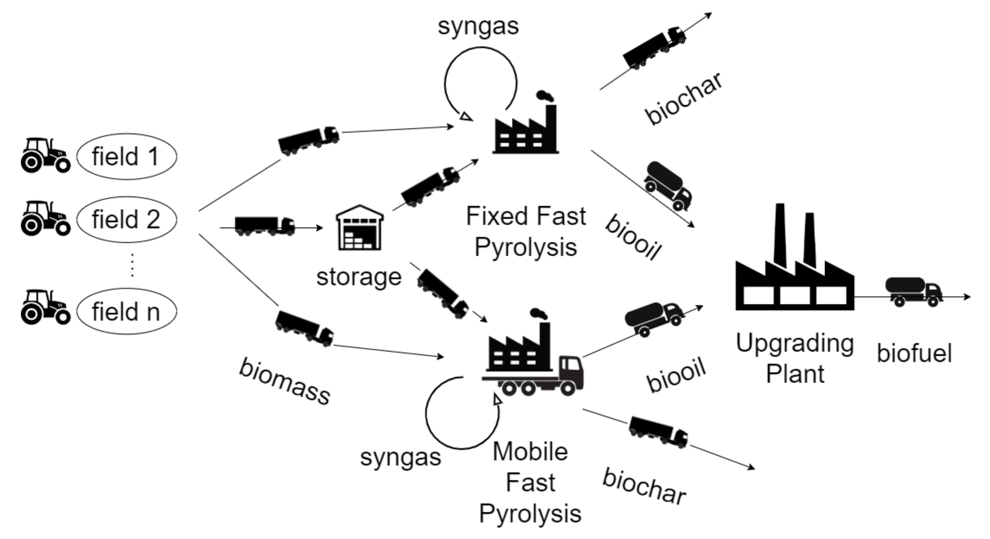
3.1. Conceptual Model Design
- Biomass flows from fields to MFP and FFP units.
- Biomass flow from fields to storage sites.
- Biomass flows from storage to MFP and FFP units.
- Bio-oil flow from FFP to FU unit.
- Bio-oil flow from MFP to FU unit.
- Biochar outputs from FFP and MFP units.
- Syngas outputs from FFP and MFP units (used internally in the fast pyrolysis process to supplement the required process heat).
- Biofuel output from FU unit.
- Biomass fields, where biomass can be planted, harvested and collected.
- Intermediate storage facilities, where biomass can be stored for later usage.
- FFP facilities of varying capacity, where biomass can be converted to bio-oil, biochar and pyrolysis gas.
- MFP facilities having the relocation capability, where biomass can be converted to bio-oil, biochar and pyrolysis gas.
- FU facilities of varying capacity, where the bio-oil from the fast pyrolysis conversion process is transformed to biofuel (end product).
- coordinates of all sites and nodes for the calculation of the intra-node distances
- annual biomass growth curve profile
- selling price of biochar and biofuel
- cost of biomass harvesting/purchasing
- cost of biomass pretreating/drying before the fast pyrolysis processes
- conversion factors from biomass to bio-oil and biochar, and from bio-oil to biofuel
- technical minimum and maximum for the facilities’ capacity
- capital and operating costs of facilities
- insurance and maintenance costs of facilities
- biomass storage cost
- cost of transporting biomass with trailer trucks and bio-oil with tanker trucks
- (a)
- the harvesting schedule for biomass at each field,
- (b)
- the number, capacity and location of the FFP and FU facilities and their processing schedule,
- (c)
- the total number of MFP facilities and their routing schedule,
- (d)
- the monthly material flows throughout the supply chain and
- (e)
- the storage capacity and inventory levels on a monthly basis
3.2. Model Formulation
3.2.1. Philosophy and Description
3.2.2. Objective Function
- annualized investment costs of facilities (AIC),
- transportation costs for biomass and bio-oil (TC),
- processing costs for conversion in fast pyrolysis and in upgrading facilities (CC),
- inventory handling cost in storage facilities (SC),
- maintenance and insurance costs of the various facilities (MIC),
- biomass harvesting/purchasing cost (BC).
- the biomass from the fields to the FFP facilities Equation (18)
- the biomass from the fields to the MFP facilities Equation (19)
- the biomass from the fields to the storage facilities Equation (20)
- the biomass from the storage facilities to the FFP facilities Equation (21)
- the biomass from the storage facilities to the MFP facilities Equation (22)
- the bio-oil from the FFP to the FU facilities Equation (23)
- the bio-oil from the MFP to the FU facilities Equation (24)
- the total relocation cost of the MFP facilities Equation (25)
3.2.3. Constraints and Equations
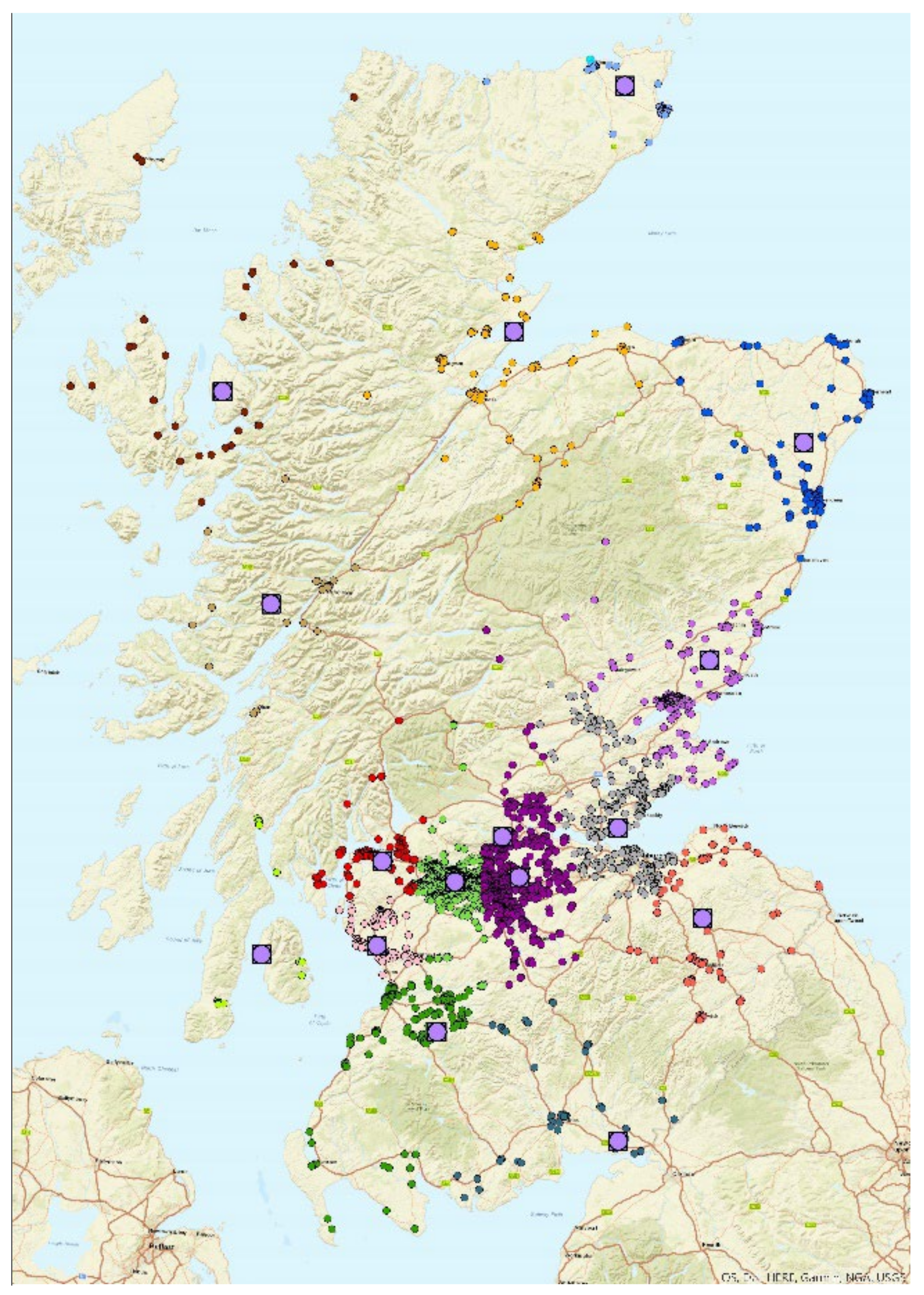
3.3. Case Study
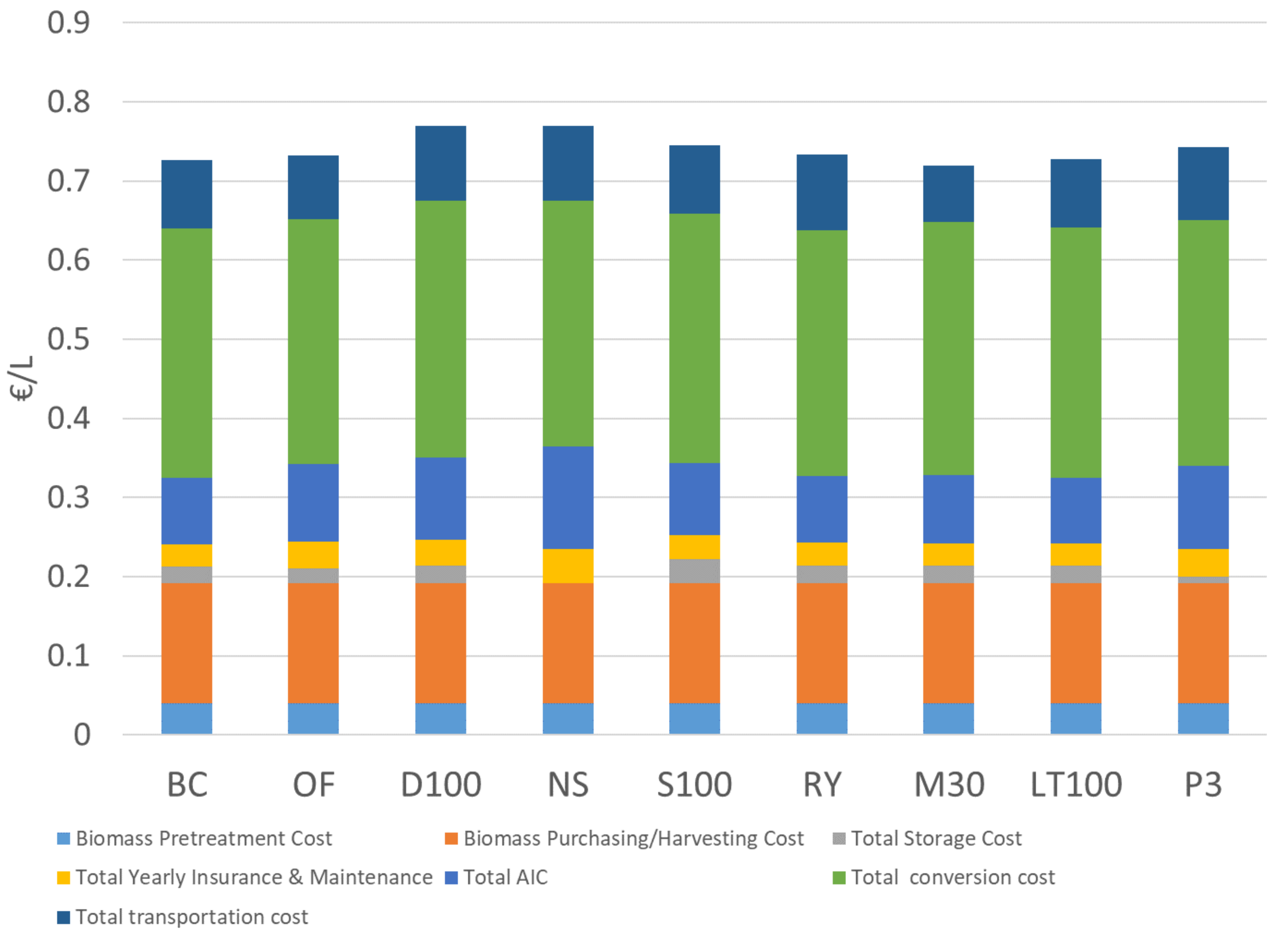
4. Results
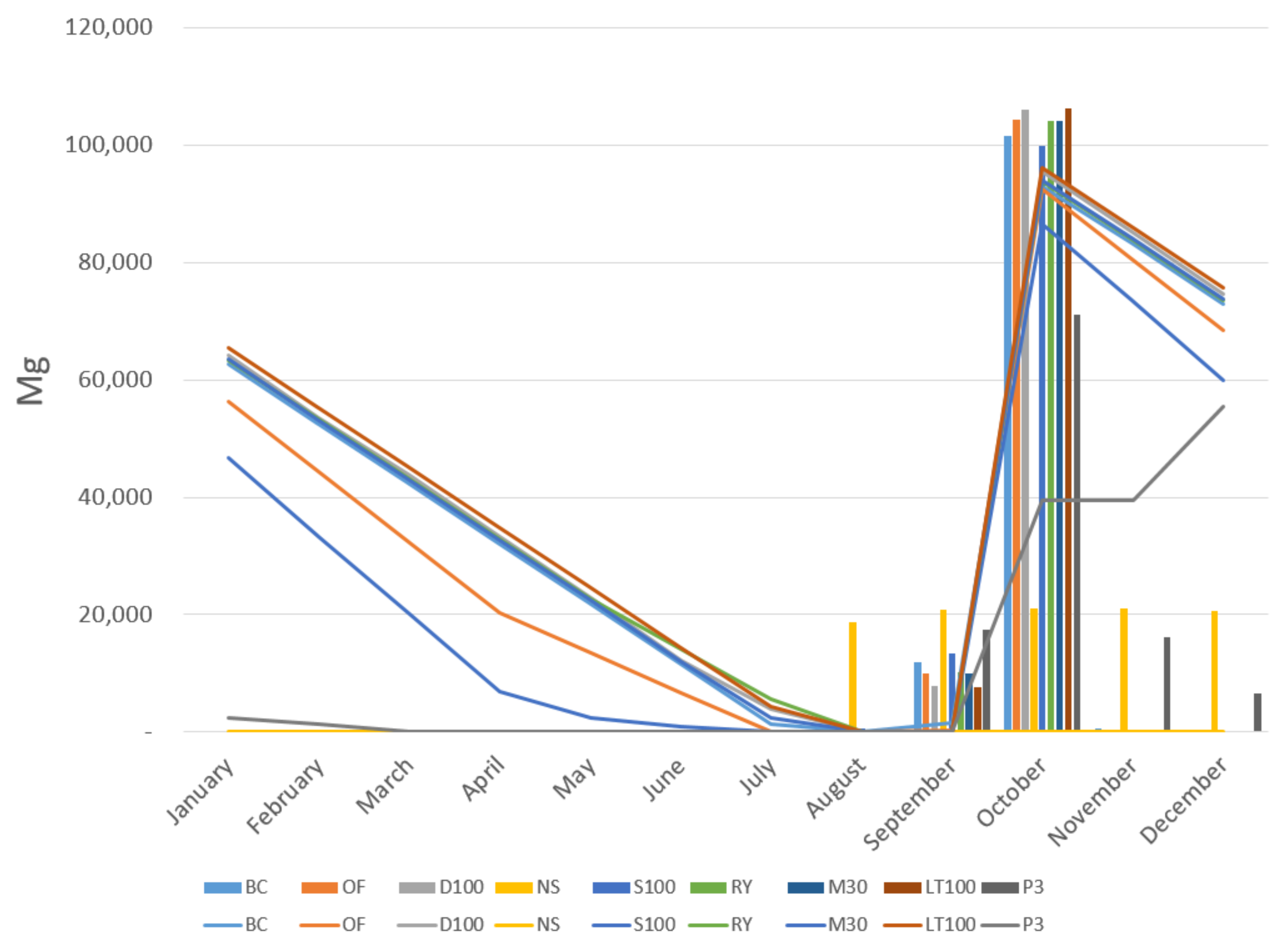
4.1. Scenarios and Inputs
- 1.
- Scenario base case (BC)—The BC scenario has full degrees of freedom to select the optimal mix of fixed and mobile facilities.
- 2.
- Scenario only fixed (OF)—The OF scenario represents the typical centralized biomass supply chain scheme without the existence of mobile facilities.
- 3.
- Scenario double distance (D100)—The D100 scenario stems from BC but the transportation cost is augmented by 100%.
- 4.
- Scenario no storage (NS)—The NS scenario stands without the warehouse option
- 5.
- Scenario double storage cost (S100)—The S100 scenario stems from BC but with an increased storage cost by 100%.
- 6.
- Scenario reduced yields (RY)—The RY scenario considers smaller yields at MFP compared to FFP facilities, namely 51% for bio-oil and 25% for biochar.
- 7.
- Scenario reduced MFP investment by 30% (M30)—The M30 scenario investigates the effect of a reduced investment cost of MFP facilities.
- 8.
- Scenario double MFP’s lifetime (LT100)—The LT100 scenario considers MFP and FFP facilities having the same lifetime of 20 years, thus reducing the related annualized costs.
- 9.
- Scenario storage three month perish (P3)—The P3 scenario allows a maximum biomass storage time of three months.
4.2. Optimization Outcomes
5. Discussion
6. Conclusions
Author Contributions
Funding
Data Availability Statement
Conflicts of Interest
Nomenclature
| Sets | |
| brp | Set of breakpoints for the investment cost curve of FFP facility |
| bru | Set of breakpoints for the investment cost curve of FU facility |
| f | Set of all fields |
| m, m′ | Set of candidate locations for the relocation of MFP facilities |
| n | Set of all nodes in the supply chain superstructure |
| p | Set of candidate locations for FFP facilities |
| s | Set of candidate location for storage facilities |
| t | Set of monthly time periods |
| u | Set of candidate locations for FU facilities |
| v | Set of MFP facilities (vehicles) |
| Parameters | |
| Total annualized investment costs (EUR) | |
| Area of field f (ha) | |
| Total biomass purchasing/harvesting cost (EUR/yr) | |
| Total conversion cost (EUR/yr) | |
| Conversion cost of FFP facilities (EUR/yr) | |
| Conversion cost of FU facilities (EUR/yr) | |
| Conversion cost of MFP facilities (EUR/yr) | |
| Purchasing cost of MFP facility (EUR) | |
| Cost of purchasing/harvesting biomass (EUR/tdry-biomass) | |
| Conversion cost in FFP facility (EUR/tdry-biomass) | |
| Conversion cost in FU facility (EUR/tbiofuel) | |
| Conversion cost in MFP facility (EUR/tdry-biomass) | |
| Cost of transporting MFP for 1 km (EUR/km) | |
| Cost of transporting 1 ton of bio-oil for 1 km (EUR/t km) | |
| Cost of transporting 1 ton of biomass for 1 km (EUR/t km) | |
| Distance between nodes (km) | |
| Height of storage facility (m) | |
| Storage cost per ton of biomass per month (EUR/tdry-biomass/month) | |
| Total investment cost of FFP facilities (EUR) | |
| Total investment cost of FU facilities (EUR) | |
| Total investment cost of MFP facilities (EUR) | |
| Capacity of MFP facility (tdry-biomass/month) | |
| Lifetime of FFP facility (yr) | |
| Lifetime of FU facility (yr) | |
| Lifetime of MFP facility (yr) | |
| A sufficiently big enough number for the Big-M linearization method | |
| Cost breakpoint values of the FFP facility in the capacity/cost curve (EUR) | |
| Break points of the capacity per month/cost curve of the FFP facility (tdry-biomass) | |
| Break points of the FU facility cost in the capacity/cost curve (EUR) | |
| Βreak points of the capacity per month/cost curve of the FU facility (tbio-oil) | |
| Selling price of biochar (EUR) | |
| Selling price of biofuel (EUR) | |
| Biomass availability at time period t (tdry-biomass/ha) | |
| Biochar revenue (EUR/yr) | |
| Biofuel revenue (EUR/yr) | |
| Discount rate (%) | |
| Total transportation cost (EUR/yr) | |
| Transportation cost of biomass from fields to MFP facilities (EUR/yr) | |
| Transportation cost of biomass from fields to FFP facilities (EUR/yr) | |
| Transportation cost of biomass from fields to storage facilities (EUR/yr) | |
| Total relocation cost of MFP facilities (EUR/yr) | |
| Transportation cost of bio-oil from MFP to FU facilities (EUR/yr) | |
| Transportation cost of bio-oil from FFP to FU facilities (EUR/yr) | |
| Transportation cost of biomass from storage to MFP facilities (EUR/yr) | |
| Transportation cost of biomass from storage to FFP facilities (EUR/yr) | |
| Conversion factor of biomass to biochar in FFP facility (tbiochar/tdry-biomass) | |
| Conversion factor of biomass to biochar in MFP facility (tbiochar/tdry-biomass) | |
| Conversion factor of bio-oil to biofuel in FU facility (tbiofuel/tbio-oil) | |
| Conversion factor of biomass to bio-oil in FFP facility (tbio-oil/tdry-biomass) | |
| Conversion factor of biomass to bio-oil in MFP facility (tbio-oil/tdry-biomass) | |
| Moisture content of biomass (%) | |
| Biomass bulk density (tdry-biomass/m3) | |
| Annual maintenance costs of FFP facilities (% of investment) | |
| Annual maintenance costs of FU facilities (% of investment) | |
| Annual insurance costs (% of investment) | |
| Annual maintenance costs of MFP facilities (% of investment) | |
| Binary variables | |
| 1 if field f is harvested at time period t, 0 otherwise | |
| 1 if MFP facility v is relocated from mobile candidate location m to m′ at time period t, 0 otherwise | |
| 1 if MFP facility v is located at candidate mobile location m at time period t, 0 otherwise | |
| 1 if FFP facility p is established, 0 otherwise | |
| 1 if storage facility s is established, 0 otherwise | |
| 1 if FU facility u is established, 0 otherwise | |
| 1 if MFP facility v is used, 0 otherwise | |
| Auxiliary binary variable for piecewise linearization of cost of FFP facility | |
| Auxiliary binary variable for piecewise linearization of cost of FU facility | |
| Continuous variables | |
| Storage area of storage facility s (m2) | |
| Amount of biomass stored at storage facility s at time period t (tdry-biomass) | |
| Capacity of FFP facility p (tdry-biomass/month) | |
| Capacity of FU facility u (tbio-oil/month) | |
| Amount of biomass transported from field f to MFP facility v at location m at time period t (tdry-biomass) | |
| Amount of biomass transported from field f to FFP facility p at time period t (tdry-biomass) | |
| Amount of biomass transported from field f to storage facility s at time period t (tdry-biomass) | |
| Amount of bio-oil transported from MFP facility v at location m to FU u at time period t (tbio-oil) | |
| Amount of bio-oil transported from FFP facility p to FU facility u at time period t (tbio-oil) | |
| Amount of biomass transported from storage facility s to MFP facility v at location m at time period t (tdry-biomass) | |
| Amount of biomass transported from storage facility s to FFP facility p at time period t (tdry-biomass) | |
| Auxiliary continuous variable for the piecewise linearization of FFP facility cost (0,1) | |
| Auxiliary continuous variable for the piecewise linearization of FU facility cost (0,1) | |
References
- Goldemberg, T.; Johansson, J. World Energy Assessment Overview 2004; United Nations Development Programme: New York, NY, USA, 2004. [Google Scholar]
- European Parliament and Council. Directive 2001/77/EC on the Promotion of Electricity Produced from Renewable Energy Sources in the Internal Energy Market. Off. J. 2001, 6, 12–25. [Google Scholar]
- United Nations Framework Convention on Climate Change. Long-Term Low Greenhouse Gas Emission Development Strategy of the European Union and Its Member States; UNFCCC: Bonn, Germany, 2020; Volume 2019, pp. 1–7. Available online: http://www4.unfccc.int/submissions/INDC/PublishedDocuments/Latvia/1/LV-03-06-EUINDC.pdf (accessed on 25 May 2022).
- EP. The European Green Deal-European Parliament Resolution of 15 January 2020 on the European Green Deal (2019/2956(RSP)). 2019. Available online: https://www.europarl.europa.eu/doceo/document/TA-9-2020-0005_EN.html (accessed on 25 May 2022).
- International Energy Agency. Technology Roadmap: Delivering Sustainable Bioenergy; IEA: Paris, France, 2017; Volume 63, pp. 87–91.
- Leboreiro, J.; Hilaly, A.K. Biomass transportation model and optimum plant size for the production of ethanol. Bioresour. Technol. 2011, 102, 2712–2723. [Google Scholar] [CrossRef] [PubMed]
- Vitale, I.; Dondo, R.G.; González, M.; Cóccola, M.E. Modelling and optimization of material flows in the wood pellet supply chain. Appl. Energy 2022, 313, 118776. [Google Scholar] [CrossRef]
- Zimon, D.; Woźniak, J.; Domingues, P.; Ikram, M.; Kuś, H. Proposition of Improving Selected Logistics Processes of Pellet production. Int. J. Qual. Res. 2021, 15, 387–402. [Google Scholar] [CrossRef]
- Bridgwater, A.V. Review of fast pyrolysis of biomass and product upgrading. Biomass Bioenergy 2012, 38, 68–94. [Google Scholar] [CrossRef]
- Jalalifar, S.; Abbassi, R.; Garaniya, V.; Hawboldt, K.; Ghiji, M. Parametric analysis of pyrolysis process on the product yields in a bubbling fluidized bed reactor. Fuel 2018, 234, 616–625. [Google Scholar] [CrossRef]
- Bolan, N.; Hoang, S.A.; Beiyuan, J.; Gupta, S.; Hou, D.; Karakoti, A.; Joseph, S.; Jung, S.; Kim, K.-H.; Kirkham, M.; et al. Multifunctional applications of biochar beyond carbon storage. Int. Mater. Rev. 2022, 67, 150–200. [Google Scholar] [CrossRef]
- Sharifzadeh, M.; Sadeqzadeh, M.; Guo, M.; Borhani, T.N.; Konda, N.M.; Garcia, M.C.; Wang, L.; Hallett, J.; Shah, N. The multi-scale challenges of biomass fast pyrolysis and bio-oil upgrading: Review of the state of art and future research directions. Prog. Energy Combust. Sci. 2019, 71, 1–80. [Google Scholar] [CrossRef]
- Moretti, L.; Milani, M.; Lozza, G.G.; Manzolini, G. A detailed MILP formulation for the optimal design of advanced biofuel supply chains. Renew. Energy 2021, 171, 159–175. [Google Scholar] [CrossRef]
- Kwon, O.; Han, J. Waste-to-bioethanol supply chain network: A deterministic model. Appl. Energy 2021, 300, 117381. [Google Scholar] [CrossRef]
- Kwon, O.; Kim, J.; Han, J. Organic waste derived biodiesel supply chain network: Deterministic multi-period planning model. Appl. Energy 2021, 305, 117847. [Google Scholar] [CrossRef]
- Yahya, N.S.M.; Ng, L.Y.; Andiappan, V. Optimisation and planning of biomass supply chain for new and existing power plants based on carbon reduction targets. Energy 2021, 237, 121488. [Google Scholar] [CrossRef]
- Jonkman, J.; Kanellopoulos, A.; Bloemhof, J.M. Designing an eco-efficient biomass-based supply chain using a multi-actor optimisation model. J. Clean. Prod. 2019, 210, 1065–1075. [Google Scholar] [CrossRef]
- Baghizadeh, K.; Zimon, D.; Jum’A, L. Modeling and Optimization Sustainable Forest Supply Chain Considering Discount in Transportation System and Supplier Selection under Uncertainty. Forests 2021, 12, 964. [Google Scholar] [CrossRef]
- Allman, A.; Lee, C.; Martín, M.; Zhang, Q. Biomass waste-to-energy supply chain optimization with mobile production modules. Comput. Chem. Eng. 2021, 150, 107326. [Google Scholar] [CrossRef]
- Albashabsheh, N.T.; Stamm, J.L.H. Optimization of lignocellulosic biomass-to-biofuel supply chains with mobile pelleting. Transp. Res. Part E Logist. Transp. Rev. 2019, 122, 545–562. [Google Scholar] [CrossRef]
- Albashabsheh, N.T.; Stamm, J.L.H. Optimization of lignocellulosic biomass-to-biofuel supply chains with densification: Literature review. Biomass Bioenergy 2020, 144, 105888. [Google Scholar] [CrossRef]
- Sharifzadeh, M.; Garcia, M.C.; Shah, N. Supply chain network design and operation: Systematic decision-making for centralized, distributed, and mobile biofuel production using mixed integer linear programming (MILP) under uncertainty. Biomass Bioenergy 2015, 81, 401–414. [Google Scholar] [CrossRef] [Green Version]
- Mirkouei, A.; Haapala, K.R.; Sessions, J.; Murthy, G.S. A mixed biomass-based energy supply chain for enhancing economic and environmental sustainability benefits: A multi-criteria decision making framework. Appl. Energy 2017, 206, 1088–1101. [Google Scholar] [CrossRef]
- Paolucci, N.; Bezzo, F.; Tugnoli, A. A two-tier approach to the optimization of a biomass supply chain for pyrolysis processes. Biomass Bioenergy 2016, 84, 87–97. [Google Scholar] [CrossRef]
- You, F.; Wang, B. Life Cycle Optimization of Biomass-to-Liquid Supply Chains with Distributed–Centralized Processing Networks. Ind. Eng. Chem. Res. 2011, 50, 10102–10127. [Google Scholar] [CrossRef]
- Wu, J.; Zhang, J.; Yi, W.; Cai, H.; Li, Y.; Su, Z. Agri-biomass supply chain optimization in north China: Model development and application. Energy 2021, 239, 122374. [Google Scholar] [CrossRef]
- Razm, S.; Nickel, S.; Sahebi, H. A multi-objective mathematical model to redesign of global sustainable bioenergy supply network. Comput. Chem. Eng. 2019, 128, 1–20. [Google Scholar] [CrossRef]
- Razak, N.H.; Hashim, H.; Yunus, N.A.; Klemeš, J.J. Integrated GIS-AHP optimization for bioethanol from oil palm biomass supply chain network design. Chem. Eng. Trans. 2021, 83, 571–576. [Google Scholar] [CrossRef]
- Winston, W.L.; Goldberg, J.B. Operations Research: Applications and Algorithms; Belmont: Nashville, TN, USA, 2004; Volume 73. [Google Scholar]
- Tan, W.; Khoshnevis, B. A linearized polynomial mixed integer programming model for the integration of process planning and scheduling. J. Intell. Manuf. 2004, 15, 593–605. [Google Scholar] [CrossRef]
- SVDLS. Scottish Vacant and Derelict Land Survey. 2021. Available online: https://www.gov.scot/publications/scottish-vacant-and-derelict-land-survey---site-register/ (accessed on 25 November 2021).
- Mos, M.; Robson, P.R.H.; Buckby, S.; Hastings, A.F.; Helios, W.; Jama-Rodzeńska, A.; Kotecki, A.; Kalembasa, D.; Kalembasa, S.; Kozak, M.; et al. Seasonal Dynamics of Dry Matter Accumulation and Nutrients in a Mature Miscanthus × giganteus Stand in the Lower Silesia Region of Poland. Agronomy 2021, 11, 1679. [Google Scholar] [CrossRef]
- Sustainable Energy Authority of Ireland. Miscanthus Factsheet. 2013, p. 4. Available online: https://www.ifa.ie/wp-content/uploads/2013/10/Miscanthus-Factsheet-SEAI.pdf (accessed on 25 May 2022).
- Ben Fradj, N.; Jayet, P.-A. Impacts of promoting perennial crops in the French agriculture. In Proceedings of the EAAE 2011, Zurich, Switzerland, 30 August–2 September 2011; pp. 1–10. [Google Scholar]
- Van der Meulen, S.; Grijspaardt, T.; Mars, W.; van der Geest, W.; Roest-Crollius, A.; Kiel, J. Cost Figures for Freight Transport—Final Report; Research to Progress; Panteia: Zoetermeer, The Netherlands, 2020; pp. 1–85. [Google Scholar]
- Rentizelas, A.; Tolis, A.; Tatsiopoulos, I.P. Logistics issues of biomass: The storage problem and the multi-biomass supply chain. Renew. Sustain. Energy Rev. 2009, 13, 887–894. [Google Scholar] [CrossRef] [Green Version]
- Singh, A.; Nanda, S.; Guayaquil-Sosa, J.F.; Berruti, F. Pyrolysis of Miscanthus and characterization of value-added bio-oil and biochar products. Can. J. Chem. Eng. 2020, 99, S55–S68. [Google Scholar] [CrossRef]
- United Nations Industrial Development Organization. Market Analysis of Biochar Produced by Small-Scale Pyrolysis Units in Vietnam; United Nations Industrial Development Organization: Vienna, Austria, 2021. [Google Scholar]


| Description | Value | Reference |
|---|---|---|
| Trailer truck transportation cost | 0.336 EUR/Mg km | [35] |
| Tanker truck transportation cost | 0.127 EUR/Mg km | [35] |
| Relocation cost | 2.66 EUR/km | [35] |
| Unitary storage cost | 2 EUR/Mg month | Est. from [36] |
| Storage max capacity | 30,000 m2 | Assumed |
| Storage max height | 5 m | [13] |
| Bio-oil yield (FFP or MFP) | 58% | [37] |
| Biochar yield (FFP or MFP) | 25% | [37] |
| Biofuel yield (FU) | 55% | [22] |
| Biofuel price | 1000 EUR/Mg | Est. from 2015 average diesel price |
| Biochar price | 250 EUR/Mg | [38] |
| Capacity of FFP and FU | 200–2000 Mg/d | [22] |
| Capacity of MFP | 50 Mg/d | [22] |
| Lifetime of fixed facilities | 20 yrs | [22] |
| Lifetime of mobile facilities | 10 yrs | [22] |
| Moisture Content | 20% | Est. from [29] |
| Bulk Density | 100 kg/m3 | Est. from [29] |
| Harvesting cost | 57.6 EUR/Mg | [24] |
| Forced drying cost | 15 EUR/Mg | [13] |
| Insurance and Maintenance | 4% of investment | [22] |
| BC | OF | D100 | NS | S100 | RY | M30 | LT100 | P3 | |
|---|---|---|---|---|---|---|---|---|---|
| Dry biomass production (Mg) | 114,020 | 114,256 | 113,867 | 102,067 | 113,723 | 114,256 | 114,252 | 114,363 | 111,414 |
| No. FFP | 1 | 3 | 1 | 2 | 1 | 3 | 1 | 1 | 2 |
| No. MFP | 1 | 0 | 3 | 0 | 1 | 0 | 2 | 1 | 0 |
| No. FU | 1 | 1 | 1 | 1 | 1 | 1 | 1 | 1 | 1 |
| Biomass processing capacity per month | 10,252 | 18,740 | 10,500 | 29,224 | 13,310 | 18,740 | 10,285 | 10,220 | 21,071 |
| Bio-oil processing capacity per month | 6018 | 7106 | 6105 | 12,356 | 7823 | 7106 | 6008 | 6000 | 10,583 |
| Average annual utilization of FFP and MFP | 93% | 51% | 90% | 29% | 71% | 51% | 93% | 93% | 44% |
| Average utilization of FU | 50% | 43% | 50% | 22% | 39% | 43% | 51% | 51% | 28% |
| Total Cost (MM EUR) | EUR 31.48 | EUR 31.76 | EUR 33.30 | EUR 29.84 | EUR 32.19 | EUR 31.76 | EUR 31.22 | EUR 31.61 | EUR 31.44 |
| Total Revenue (MM EUR) | EUR 44.02 | EUR 44.22 | EUR 43.76 | EUR 39.50 | EUR43.91 | EUR 44.22 | EUR 44.02 | EUR 44.15 | EUR 43.12 |
| Total Profit (MM EUR) | EUR 12.54 | EUR 12.46 | EUR 10.46 | EUR 9.66 | EUR11.72 | EUR 12.46 | EUR 12.80 | EUR 12.54 | EUR 11.68 |
| Biofuel cost (EUR/L) | 0.73 | 0.73 | 0.77 | 0.77 | 0.75 | 0.73 | 0.72 | 0.73 | 0.74 |
| Difference of profit against BC | 0 | −0.66% | −16.62% | −22.96% | −6.50% | −0.66% | 2.07% | 0.03% | −6.88% |
| BC | OF | D100 | NS | S100 | RY | M30 | LT100 | P3 | |
|---|---|---|---|---|---|---|---|---|---|
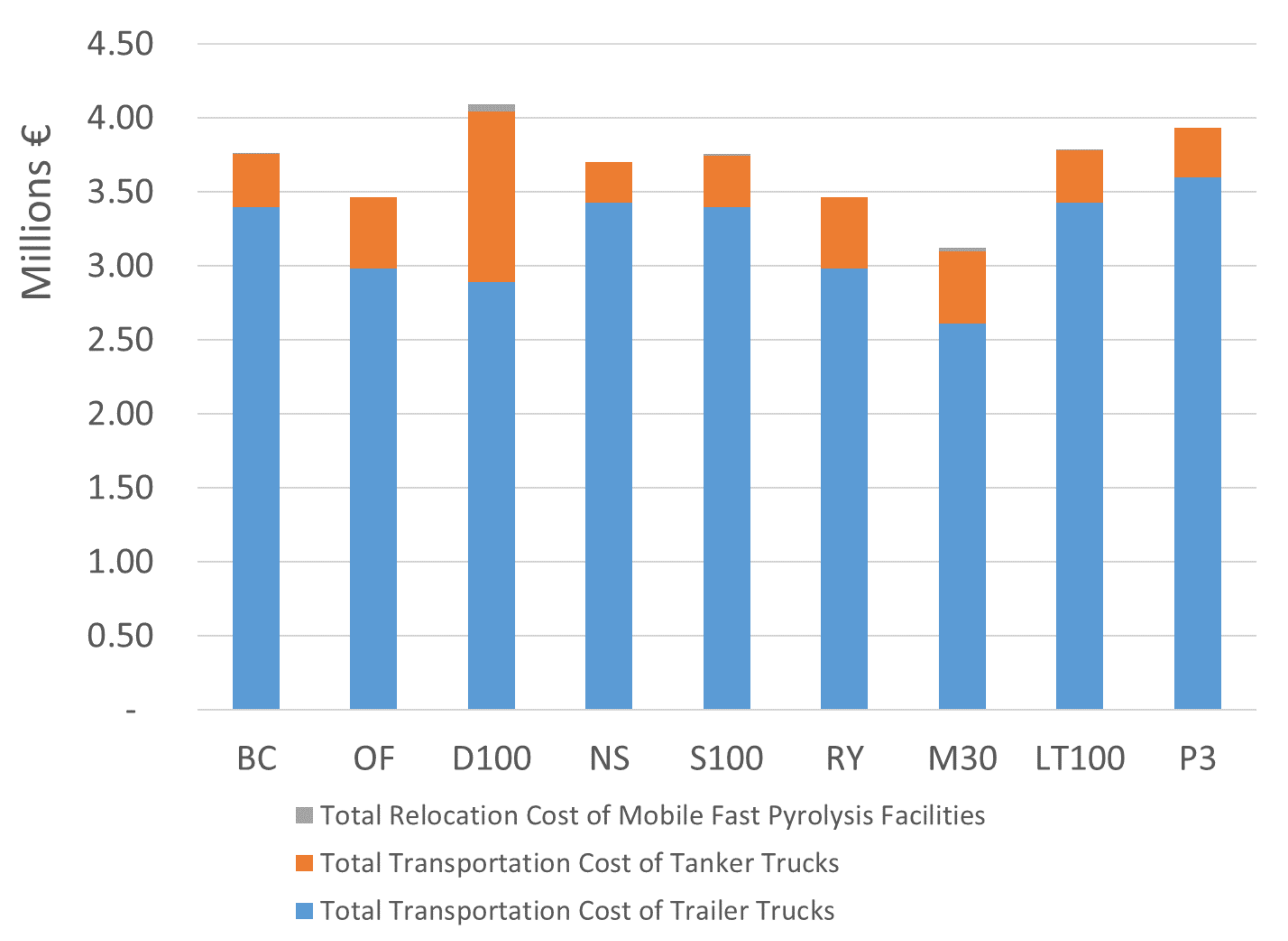
| Percentage of relocation to total transportation cost | 0.19% | N/A | 1.17% | N/A | 0.33% | N/A | 0.71% | 0.20% | N/A |
| Percentage of relocation to total cost | 0.02% | N/A | 0.14% | N/A | 0.04% | N/A | 0.07% | 0.02% | N/A |
Publisher’s Note: MDPI stays neutral with regard to jurisdictional claims in published maps and institutional affiliations. |
© 2022 by the authors. Licensee MDPI, Basel, Switzerland. This article is an open access article distributed under the terms and conditions of the Creative Commons Attribution (CC BY) license (https://creativecommons.org/licenses/by/4.0/).
Share and Cite
Psathas, F.; Georgiou, P.N.; Rentizelas, A. Optimizing the Design of a Biomass-to-Biofuel Supply Chain Network Using a Decentralized Processing Approach. Energies 2022, 15, 5001. https://doi.org/10.3390/en15145001
Psathas F, Georgiou PN, Rentizelas A. Optimizing the Design of a Biomass-to-Biofuel Supply Chain Network Using a Decentralized Processing Approach. Energies. 2022; 15(14):5001. https://doi.org/10.3390/en15145001
Chicago/Turabian StylePsathas, Fragkoulis, Paraskevas N. Georgiou, and Athanasios Rentizelas. 2022. "Optimizing the Design of a Biomass-to-Biofuel Supply Chain Network Using a Decentralized Processing Approach" Energies 15, no. 14: 5001. https://doi.org/10.3390/en15145001