Long-Term Evaluation of Comfort, Indoor Air Quality and Energy Performance in Buildings: The Case of the KTH Live-In Lab Testbeds

Abstract

Digitalization offers new, unprecedented possibilities to increase the energy efficiency and improve the indoor conditions in buildings in a cost-efficient way. Smart buildings are seen by many stakeholders as the way forward. Smart buildings feature advanced monitoring and control systems that allow a better control of the buildings’ indoor spaces, but it is becoming evident that the massive amount of data produced in smart buildings is rarely used. This work presents a long-term evaluation of a smart building testbed for one year; the building features state-of-the-art monitoring capability and local energy generation (PV). The analysis shows room for improving energy efficiency and indoor comfort due to non-optimal control settings; for instance, average indoor temperatures in all winter months were above 24 °C. The analysis of electricity and domestic hot water use has shown a relevant spread in average use, with single users consuming approximately four times more than the average users. The combination of CO₂ and temperature sensor was sufficient to pinpoint the anomalous operation of windows in wintertime, which has an impact on energy use for space heating. Although the quantification of the impact of users on the overall energy performance of the building was beyond the scope of this paper, this study showcases that modern commercial monitoring systems for buildings have the potential to identify anomalies. The evidence collected in the paper suggests that this data could be used to promote energy-efficient behaviors among building occupants and shows that cost-effective actions could be carried out if data generated by the monitoring and control systems were used more extensively.

1. Introduction

Energy performance in buildings is critical to sustainability. New developments in Information and Communication Technology (ICT) have greatly improved the possibilities to monitor energy performance and indoor climate in buildings in a cost-efficient way. Modern buildings are incrementally getting smarter with more advanced monitoring tools, leading to increased expectations on the possibility to use the generated data to optimize the design and the energy performance of the buildings.

Smart buildings typically deploy, among others, more advanced sensor capabilities and advanced monitoring systems. Data from monitoring systems has for instance been used to monitor the energy performance of buildings during operation [1,2,3], to highlight significant energy performance gaps and to identify the reasons for these discrepancies between expected energy use from design and actual monitored energy use, [4,5,6].

Building data has also been extensively used also to map the Indoor Environmental Quality (IEQ) in the operation of buildings [7,8,9], and even in buildings built with modern control systems, issues with IEQ were found [10,11,12]. For instance, Geng et al. [10] performed a large-scale and long-term evaluation of the indoor environmental quality in 41 green office buildings in China for a timespan of one year. The study correlated the IEQ with the different investigated climate areas and found IEQ generally within the recommendations; still, several issues with thermal comfort were found, such as insufficient cooling in summer, insufficient heating in winter and overheating in winter. Monitoring systems often highlight situations that diverge from target design conditions; Hagejärd et al. [12], in a study focusing on load shifting on 33 multi-residential buildings, highlight that tenants experience too low perceived indoor temperatures and poor heating control.

Long-term monitoring campaigns can also be the basis for improving design and standards. Choi et al. [13], for instance, study IEQ conditions with data collected for seven years over 400 workstations with spot and continuous measurements and challenge the validity of current IEQ guidelines. Long-term monitoring campaigns are used, for instance, to gain a better understanding of energy use in buildings during operation and its relationship with comfort. Lawrence and Keime [14] scrutinize and compare the impact of active and passive design solutions in operation on energy use and perceived comfort in two higher-education buildings in the UK to improve the design of the buildings by means of data measurements and questionnaires.

There is increasing scientific evidence that the performance of buildings is affected by behavioral dynamics of building occupants. A study sponsored by the World Business Council for Sustainable Development [15] assesses that wasteful behavior can add one-third to a building’s designed energy performance, while conservation behavior can save a third. Hong et al. [16] highlight how occupant behavior in buildings is complex, not well understood and often oversimplified. They also report an energy saving potential up to 20% in energy-aware occupant behavior, with most effective measures being direct feedback and human-in-the-loop sensing and control. Nguyen and Aiello, in literature research reviewing both experimental and simulative studies [17], indicate HVACs along with plug loads and light as the main subsystems where energy savings can be reached in relation to occupant behavior. However, they also show that the estimated energy saving potential from user activities tend to be higher in simulations than in actual experiments. For instance, the energy saving potential estimated in HVAC simulations ranges from approximately 10 to 60%, while an actual experimental study reports it at 13%; similarly, savings for light use range from 33 to approximately 60%, while actual experiments range from 13 to 25%.

Among the challenges to quantify the impact of user behavior on building energy performance, lack of real measured data with respect to how occupants use buildings often leads to assumptions [18].

A factor that is common to all previous studies is the capability to sense, store and analyze data from the indoor environment. There is a need for more quantitative information on smart buildings at the interface between indoor environmental quality, energy and resource use and the impact of behavior, and the sensor data needed to map them. Modern buildings offer more advanced sensor measurements and data collection capabilities that potentially support a more efficient operation and continuous improvement of the design of buildings. The experimental evaluation of performance and indoor thermal comfort is often limited to short periods or focused on building subsystems [19,20,21]. However, there is a limited number of contributions that deal simultaneously with the detailed analysis of energy performance and indoor environmental quality over long-term periods from commercially available monitoring systems. This paper addresses this gap, analyzing high resolution data collected over a time span of one year in a living lab testbed with smart building features and modern design. The building is a set of three residential buildings for student accommodation, which includes 305 single room apartments. All apartments are equipped with sensors to monitor and control indoor temperature and carbon dioxide concentration; in addition, the buildings feature detailed monitoring of the heating and ventilation systems. The paper maps and analyzes IEQ parameters and the energy use in the building and scrutinizes its monitoring and control system. The primary focus of this work is to assess the capacity of a commercial, state-of-the-art monitoring system to understand whether the building is operating under acceptable indoor conditions, to assess the resource use—namely energy for space heating, use of domestic hot water and electricity consumption—and the impact of anomalies due to building occupants’ behavior in the analyzed buildings. Ultimately, the paper is aimed at elaborating considerations on: the amount of data generated in buildings and the amount that is effectively used; the building energy gap assessment; the variability of controllable resources such as domestic hot water and electricity; and the identification and impact of occupant behavior on indoor environment conditions and building energy use.

The following parts of the paper introduce the methodology (Section 2), which includes the description of the building testbeds, their technical system and the approach used to clean and filter the data collected. Results on energy performance, indoor environmental quality and indications on occupant behavior are introduced in Section 3. Section 4 discusses the results and draws considerations in relation to the envisioned development of smart buildings. Final remarks and future work are summarized in Section 5.

2. Methodology

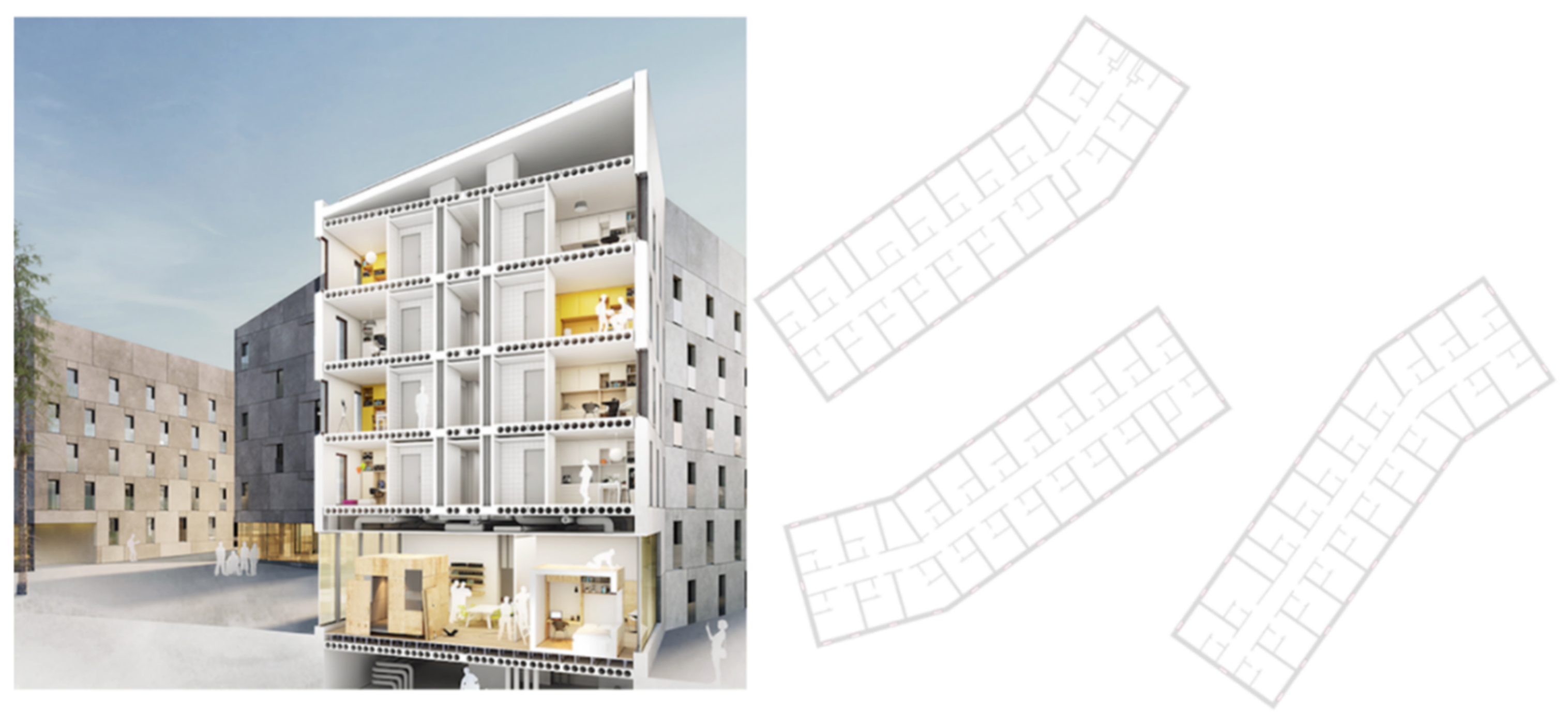
2.1. Description of the Experimental Setup

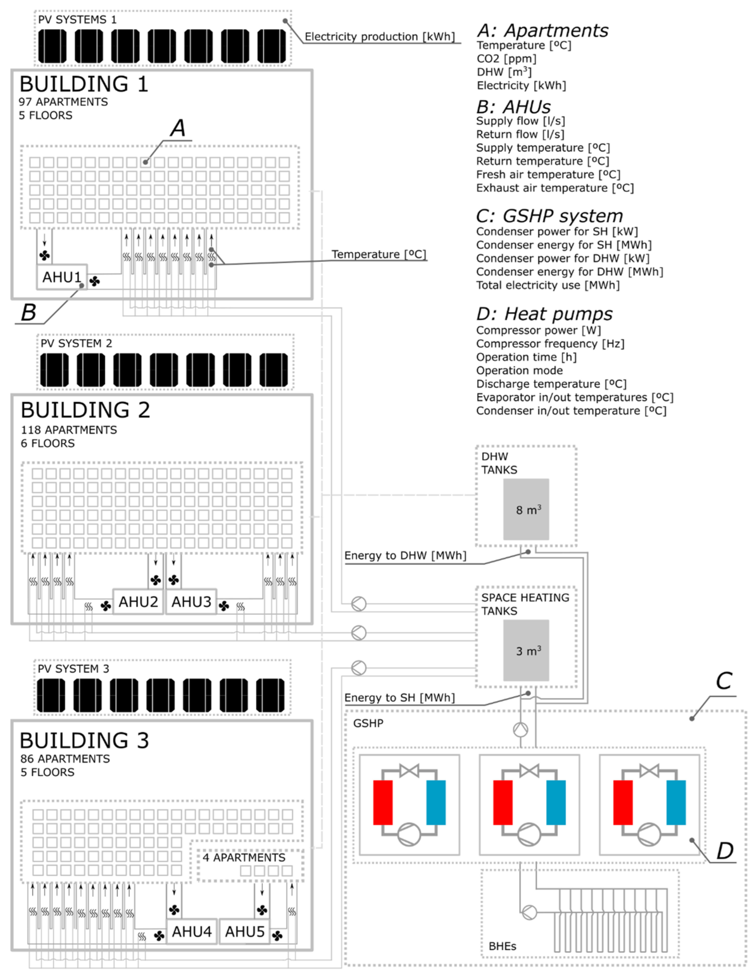
2.1.1. Testbed EM: Buildings and Apartments

The Testbed Einar Mattsson (“Testbed EM” in the following) is a set of three residential buildings including a total of 305 student apartments located at the main campus of the Royal Institute of technology (KTH) in Stockholm. The average size of the apartments is approximately 20 m², and each includes a living room, a small kitchen and a bathroom. The three buildings have a total heated area of about 10,590 m².

A set of three 60 kW geothermal heat pumps provides heat to the Testbed EM; the heat pumps use 11 water-filled boreholes as a heat source. The geothermal installation design has some unconventional features in order to function also as an infrastructure for research. The single borehole length ranges between 225 and 350 m, with a total borehole length of 3085 m. Fiber optic cables are installed in 5 boreholes to allow the monitoring of the temperature along the borehole length through a Distributed Temperature Sensing (DTS) equipment. An additional borehole with a length of 100 m is available but used only for testing and research purposes and is not coupled to the three geothermal heat pumps [22].

The buildings feature an efficient thermal envelope and the Termodeck system, an example of Thermally Activated Building Systems (TABS) for heat emission. Ventilation air circulates through the building slabs before entering the rooms, preheating or precooling the slabs; this feature allows a more stable and homogeneous temperature distribution in the indoor spaces, adding to the comfort.

The heating system of the buildings includes a heat recovery system for ventilation and for the wastewater, and 3 waste heat exchangers. In addition, renewable energy is generated locally with 667 PV panels installed on the whole roof surface, for a total of 1150 m². Figure 1 shows a 3D sideview and blueprints of typical floor in each building of Testbed EM.

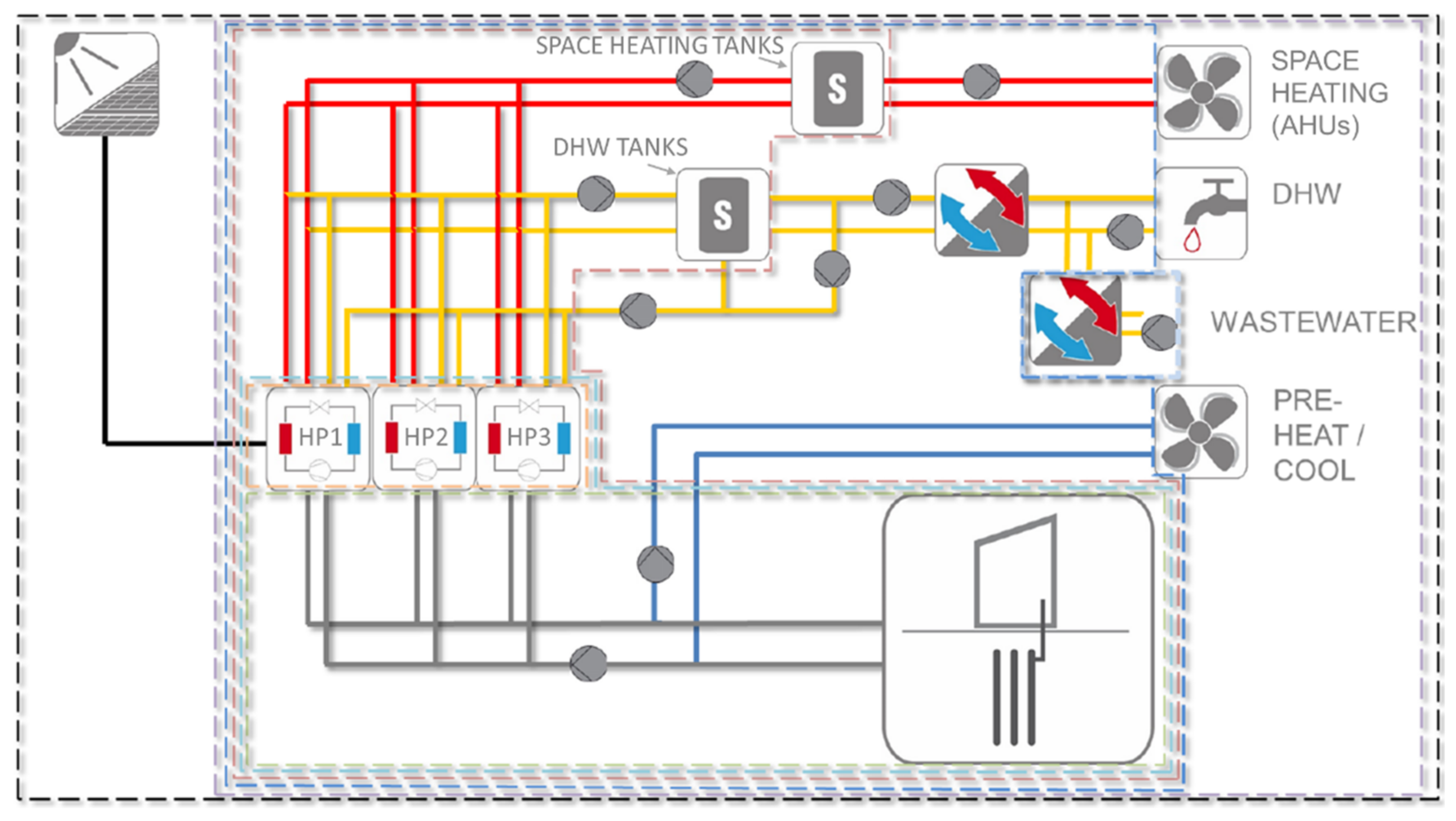
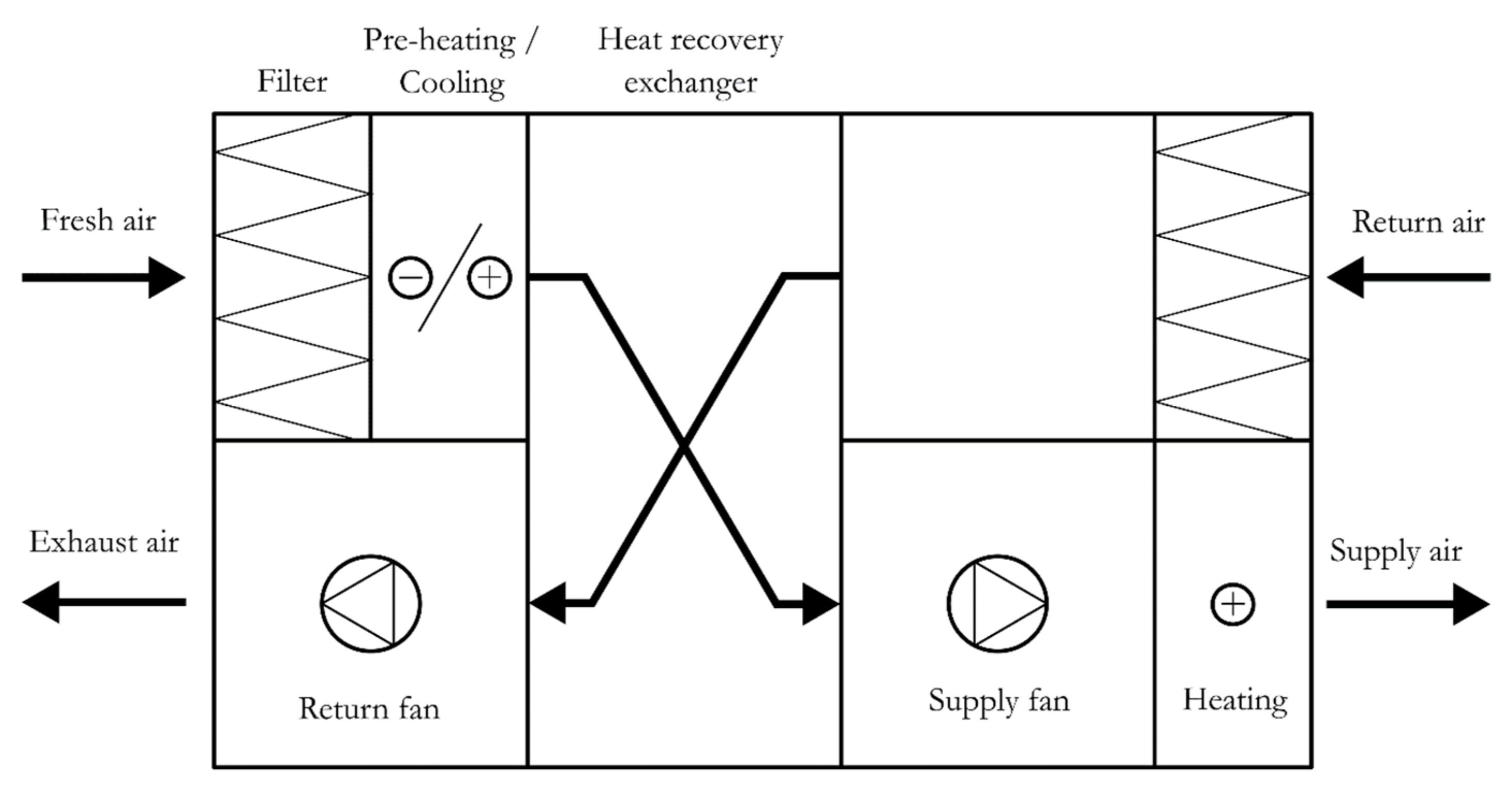
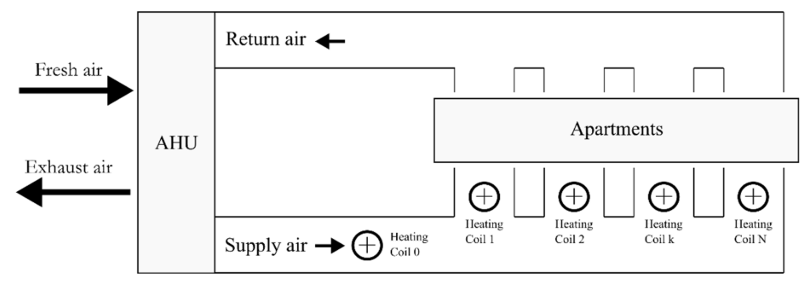
2.1.2. Testbed EM: Heat Pump, Ventilation and Monitoring Systems

The buildings are located in a cold climate and are thus heating dominated. Figure 2 shows a simplified schematic of all the sub-systems included in this study. Space heating and Domestic Hot Water (DHW) are provided via Ground Source Heat Pumps (GSHPs). The heat is supplied to the apartments through 5 centralized Air Handling Units (AHUs). Cooling is not actively provided, although free-cooling may occur via the ground. The system does not have an auxiliary heating system although heat recovery on wastewater is implemented and used to pre-heat DHW. In order to smooth out peak demand from the DHW system, 8 m³ of water tank storage are installed. Incoming fresh air to the AHUs can also be pre-heated from (or cooled by) the boreholes.

Figure 3 shows a simplified schematic of the heat pump system. There are eight series-connected water tanks on the DHW side and two water tanks on the space heating side. The volume of each water tank is 1 m³. The DHW is circulated around the building and the cold water is pre-heated with wastewater whenever possible. The circulation pumps on the source side are controlled according to a constant pressure drop setting.

Figure 4 shows a schematic of each of the 5 AHUs available in the system and Figure 5 shows a simplified scheme of the heating distribution between one AHU and the apartments. It should be noticed that one of the buildings (namely, Building 2) is equipped with two AHUs, while Building 1 and Building 3 are equipped with one AHU each. Additionally, each AHU is connected to a different number of vertical air distribution ducts, each one equipped with a heating coil installed (named “Heating Coil k” in Figure 5). As summarized in

Table 1. Heating coils of each AHU per building.

	AHU 1	AHU 2	AHU 3	AHU 4	AHU 5
Building	1	2	2	3	3
Heating coils	8	5 *	4 *	9	1

* Including an additional heating coil in the manifold.

, the AHUs of Building 2 serve 4 and 3 vertical distribution ducts and the AHUs of Building 1 and Building 3 serve 8 and 9 vertical distribution ducts, respectively. Finally, it should be noticed that the central heating coil named “Heating Coil 0” in Figure 4 is available only in the AHUs of Building 2. The AHU installed in Building 3 serves only 4 apartments that are used for research studies and are formally identified as an independent testbed, called Testbed KTH.

Figure 5 also shows a direct connection available between the boreholes and the AHUs to allow, in principle, the pre-heating or cooling of the incoming air in the AHUs.

The Testbed EM is equipped with an extensive network of sensors that covers the buildings at apartment, heat pump system and ventilation system levels. At the apartment level, the indoor thermal comfort and air quality is controlled separately in each apartment via dedicated temperature and CO₂ sensors regulating supply and return airflows. In addition, domestic hot water and electricity are measured in all apartments. A total of more than 7000 data points (including sensors, alarms and set points) are continuously logged with a sample rate of 1 min. The data analysis carried out in this paper covers the 12 months of data between July 2020 and June 2021.

Table 2. Main data points used for the data analysis presented in this paper.

Subsystem	Data Point (Description)
AHU	Air intake temperature (fresh air) Supply temperature (common) Supply temperatures (distribution levels) Return temperature (common) Supply air flow rate Return air flow rate Supply air fan power Return air fan power
Heat pump (individual unit)	Compressor power Compressor frequency Operation time Operation mode (control signal: 0 = SH, 1 = DHW) Hot gas discharge temperature Inlet evaporator (fluid side) Outlet evaporator (fluid side) Inlet condenser (fluid side) Outlet condenser (fluid side)
Heat pumps (three units aggregated)	Condenser power for space heating Condenser power for domestic hot water Condenser energy for space heating Condenser energy for domestic hot water Total electricity use (including heat pump units and borehole circulation pumps)
Apartments	Indoor temperature CO2 concentration Electricity use DHW use
Buildings	Outdoor temperature Electricity use of the freshwater pressurizer Bought electricity (3 buildings) PV electricity production (3 PV systems)
Other	Electricity use of service and laundry rooms

shows a selected list of the data points used for the data analysis presented in this paper.

2.2. Description of the Research Methodology

An extensive part of this study consisted in identifying, parsing, mapping and cleaning the available data. This section proposes examples of how the measurements of the data points of the 305 apartments were quantified and how the quality of the measurements was preliminary assessed.

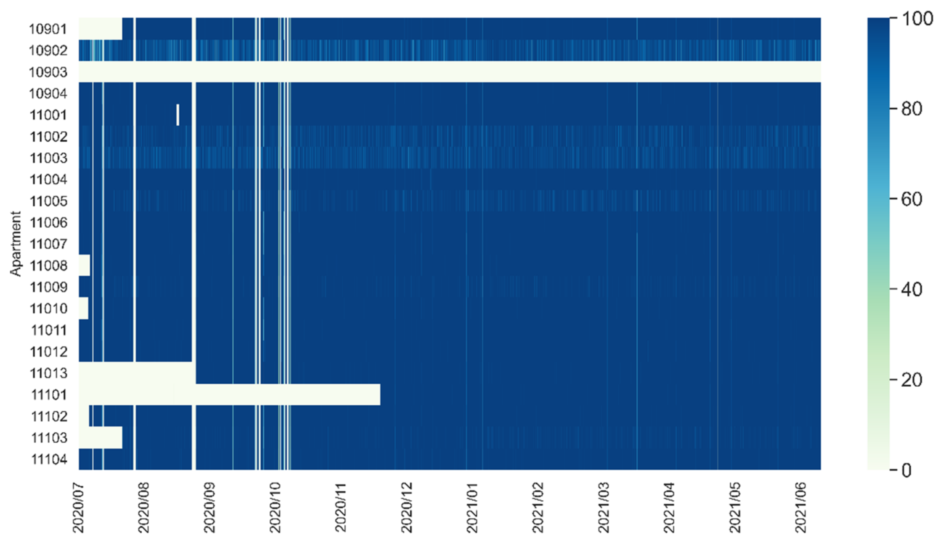
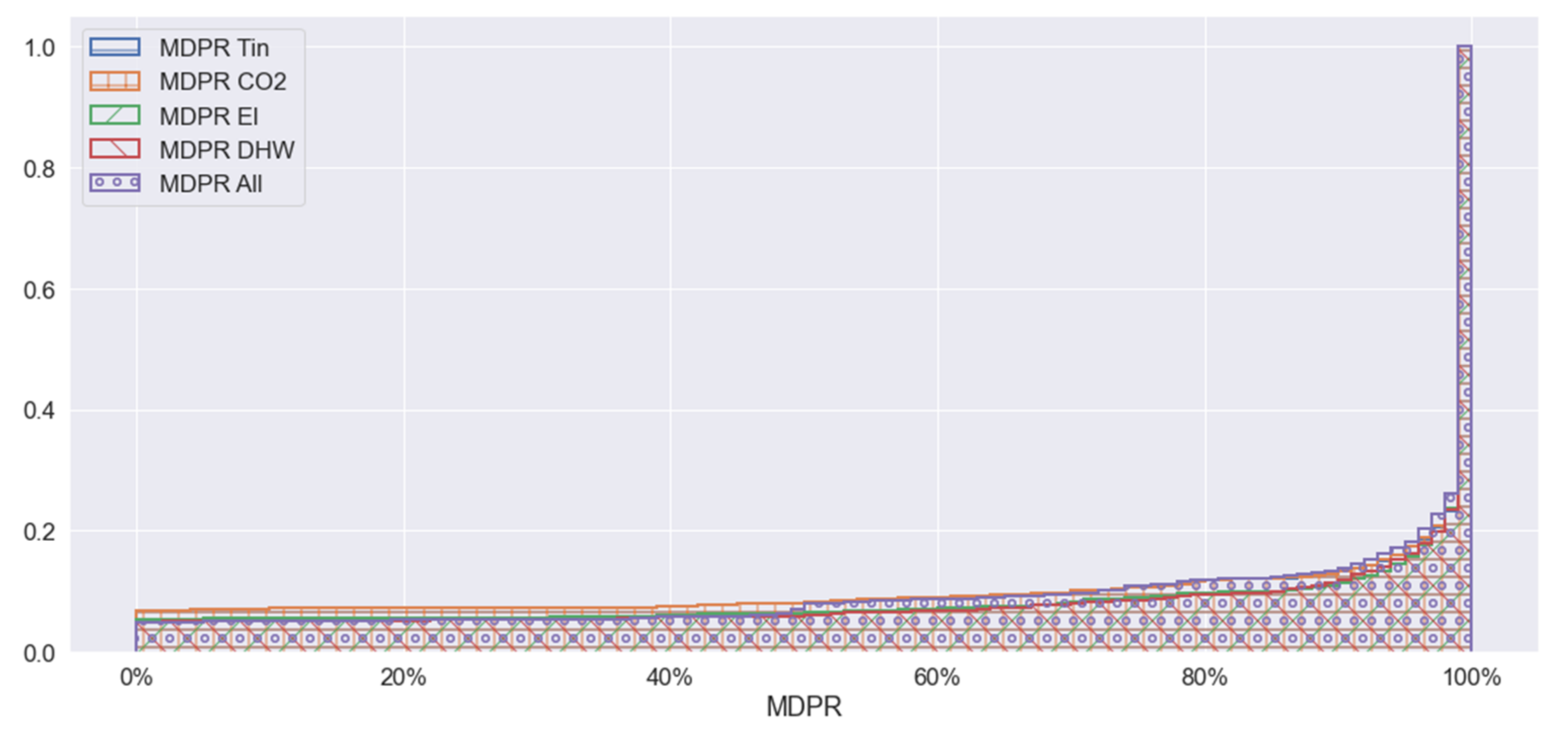
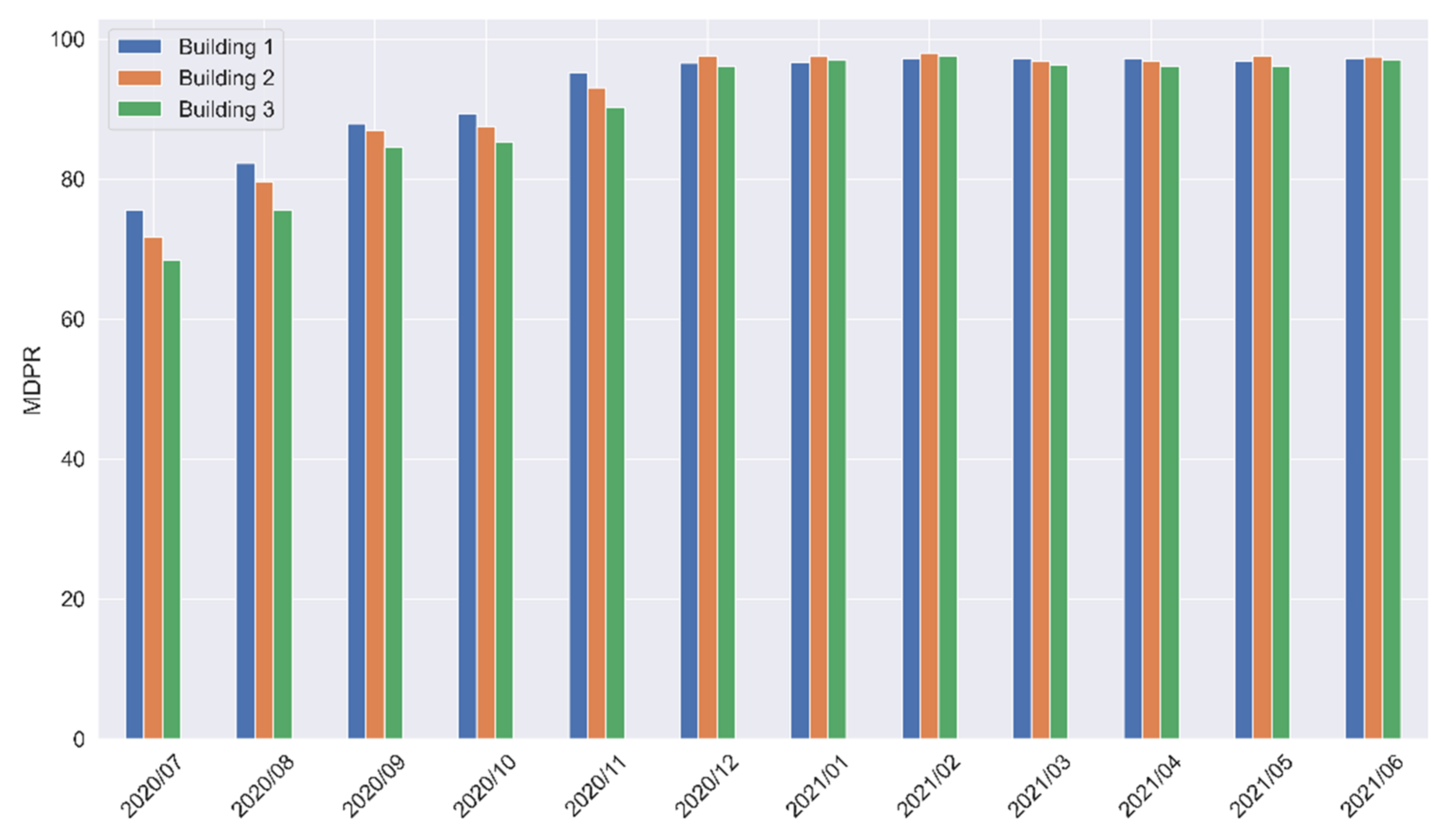
2.2.1. Data Quantity

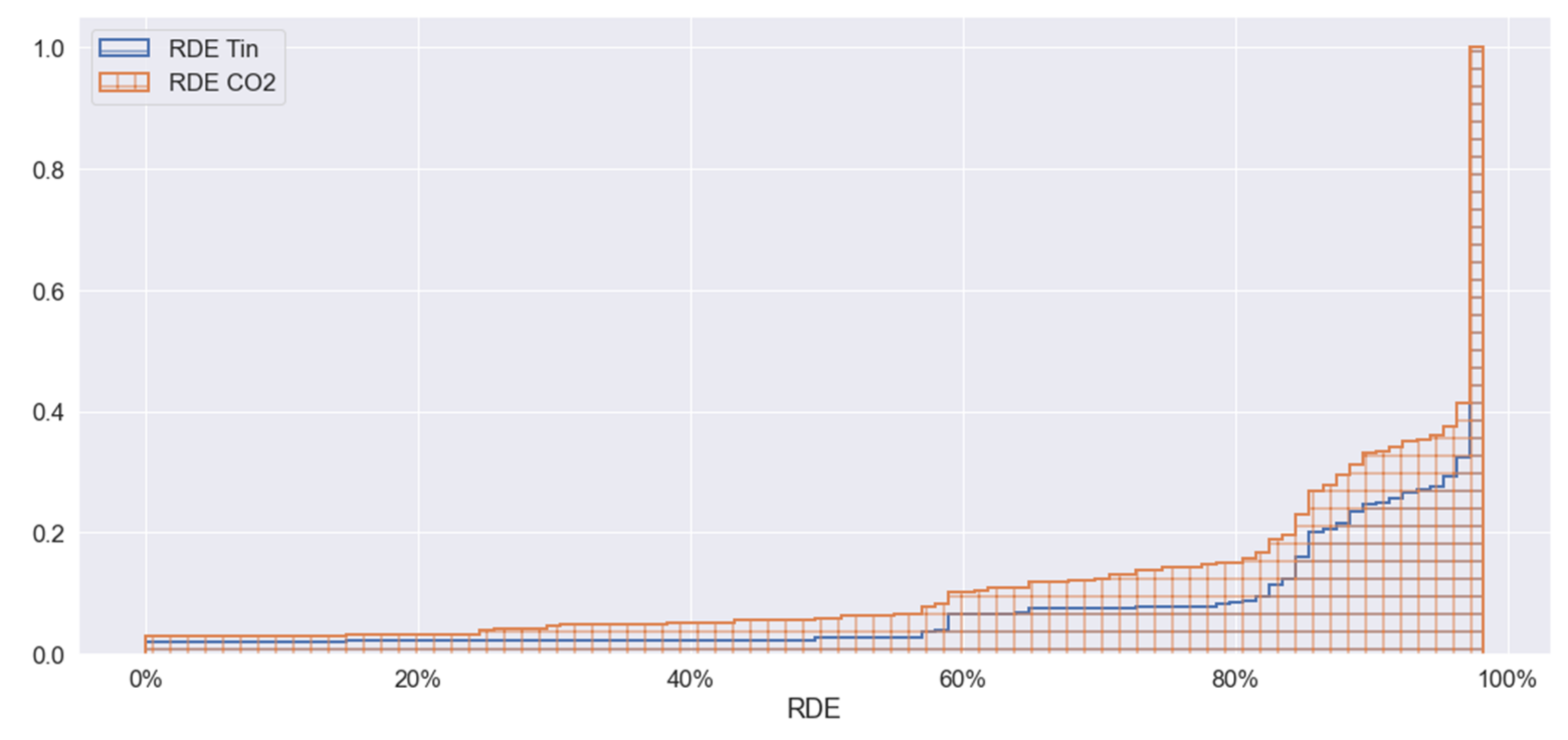
The monitoring system of Testbed EM logs indoor temperature, CO₂ concentration, electricity use and domestic hot water use in all 305 apartments with a sample rate of 1 min. An indicator, called Missed Data Points Ratio (MDPR), was defined as the available number of measurements over the expected number of measurements based on the sample rate of 1 min to quantify the data availability over the 12-month period of analysis (Equation (1)). An MDPR of 100% would indicate that all measurements are available as expected. In the presented period, the MDPR of Testbed EM is 91.3%.

$$\mathrm{MDPR}=\frac{\mathrm{available} \mathrm{number} \mathrm{of} \mathrm{measurements}}{\mathrm{expected} \mathrm{number} \mathrm{of} \mathrm{measurements}}$$

(1)

Figure 6 shows an extract of the heat map chart of the hourly MDPR generated to quickly assess the overall availability of data in each apartment. In particular, the chart shows the hourly MPDR of the indoor temperature. Indoor temperature measurements are not available for 6 apartments, including apartment 10903. Other apartments (i.e., 10901, 11013, 11101 and 11103) appear to have major data availability issues in the first part of the analyzed period. Notably, the vertical blank lines in the chart indicate general temporary disruptions of the monitoring system.

Figure 7 shows the cumulative MDPR distribution obtained considering the MDPR average of all apartments. Overall, the chart indicates a probability of about 30% to have missing at apartment level. Figure 8 shows the monthly value of MDPR per building, indicating that the majority of the missing measurements for the apartments occurred in the first months of the analyzed period.

Overall, the data points of six apartments have no data from either indoor temperature or CO₂ sensors, one apartment has no data from electricity meters while all the DHW data points provide data relative to all the apartments.

2.2.2. Data Quality

A second indicator has been used to identify the measurements of indoor temperature and CO₂ concentration outside expected and reasonable ranges. In case of indoor temperature, the filtered data includes the measurements between 10 and 40 °C, while for the CO₂ concentration, the filtered data includes the measurements between 300 and 5000 ppm. The lower limit for the CO₂ level is based on a conservative approximation of the expected average outdoor concentration [23], while the upper limit is a conservative approximation based on the CO₂ distribution in the 305 apartments. The Ratio of Data to Errors (RDE) is defined as the number of filtered measurements over the total number of expected measurements (Equation (2)).

$$\mathrm{RDE}=\frac{\mathrm{filtered} \mathrm{number} \mathrm{of} \mathrm{measurements}}{\mathrm{expected} \mathrm{number} \mathrm{of} \mathrm{measurements}}$$

(2)

Figure 9 shows the cumulative RDE calculated for indoor temperature and CO₂ concentration measurements from all 305 apartments. The figure indicates that the data points of CO₂ concentration contain more data outside the expected range compared to the indoor temperature. The inspection of the charts suggests that there is a 40% probability to have missing data or data out-of-range in the available measurements. However, it should be noted that the probability is lower than 20% if we consider 80% of measurements available and within an expected range.

Since the measurements of electricity and domestic hot water use are highly affected by user behavior, arbitrary ranges of expected values have not been defined in the first stage of this study. However, the following sections describe the results from the data analysis including also those data points, presenting the measurement distribution, the outliers and their possible interpretation.

2.2.3. Study Roadmap and Limitations

This study shows the results of the analysis of the data from Testbed EM over the 12-month period between July 2020 and June 2021. The following sections of the article include an overview of the building energy use and production, a more detailed analysis of the heat pump and ventilation systems, an overview of the net energy flows. Two subsections are dedicated to the analysis of the indoor environment using the available data points from the 305 apartments of the three buildings.

A few limitations are known beforehand:

-

Local measurements of solar irradiance are not available, and a complete performance evaluation of the PV system was therefore not possible.

-

The analysis of the energy flows at apartment level is not possible due to the lack of dedicated sensors (ventilation inlet and outlet temperature and volumetric flow meters) and corresponding data points.

-

Relative humidity sensors are not available in the apartments. A thorough and complete assessment of the indoor thermal comfort following International Standards such as the ASHRAE 55 and ISO 7730 [24,25] was therefore not possible. However, Section 3.6 and Section 3.7 propose insights based on the available measurements, including indoor temperature and CO₂ concentration.

-

A rigorous assessment of Indoor Air Quality (IAQ) as proposed in other studies [26,27,28,29] was also not possible. Measurements of SO₂, NO₂, PM_2.5 and PM₁₀ are currently not available in Testbed EM.

A summary of the shortcomings of the monitoring system and their impact on the building management is presented in the discussion section.

3. Results

3.1. Building Energy Use and Energy Production

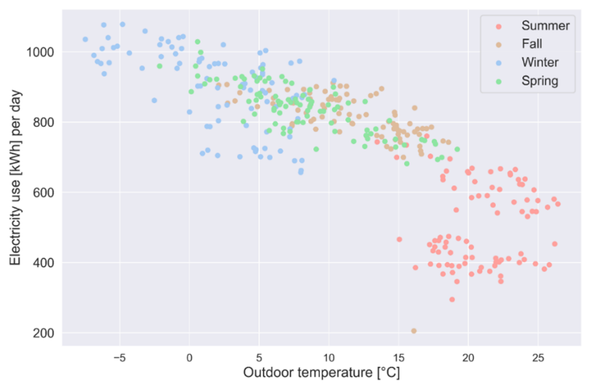
3.1.1. Energy Signature

The monitoring system of Testbed EM includes dedicated data points to account for the bought electricity for the entire facility. Figure 10 shows the daily bought electricity versus the hourly average of the outdoor temperature. As qualitatively expected from buildings with no active cooling system, the peaks of daily energy use occur in winter days.

Quantitatively, the figure shows a daily baseline use of energy of about 500 kWh/day and a peak of about 2800 kWh/day around −5 °C. The aggregated metrics provided in

Table 3. Summary table based on daily energy use of Testbed EM.

	Sum	Min	Max	Average	Median	St.Dev	Trend	Intercept
	MWh	kWh/day	kWh/day	kWh/day	kWh/day	kWh/day	kWh/day/K	kWh/day
Summer	66	494	1330	719	684	170	−18.5	1105
Fall	143	1035	2208	1575	1606	294	−61.5	2291
Winter	195	1597	2853	2171	2090	348	−69.2	2311
Spring	135	782	2304	1474	1450	344	−66.4	2025
Overall	540	494	2853	1480	1525	595	−70.1	2234

show that over summer and winter the total energy use is about 66 MWh and 195 MWh, respectively. The table includes also the linear regression coefficients calculated considering the daily values grouped by season. The inspection of the coefficients indicates that overall, a drop of 5 °C of the outdoor temperature corresponds to an increase of the energy use of about 350 kWh/day. It is also interesting to notice from Figure 10 that the daily energy use during spring days appears to be lower than during fall days for a given outdoor temperature. Although the minimum energy use during spring (782 kWh/day) is in fact about 25% lower than during fall (1036 kWh/day), the average value (1474 kWh/day) is only 6% lower (1575 kWh/day). The regression coefficients show that despite the trend during the spring being between the trends in winter and fall, the intercept values are shifted down of about 300 kWh/day (2025 kWh/day versus 2291 and 2311 kWh/day).

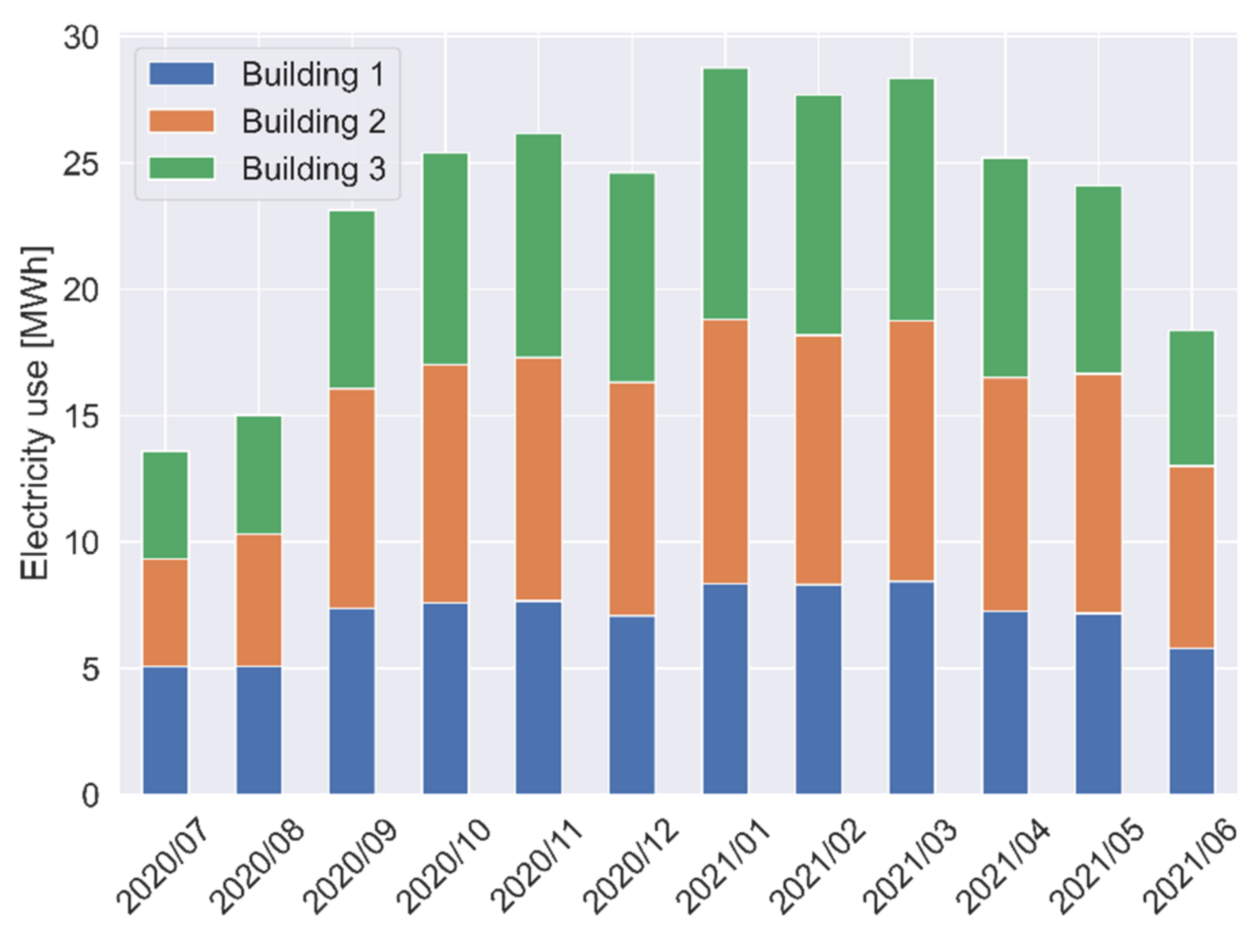
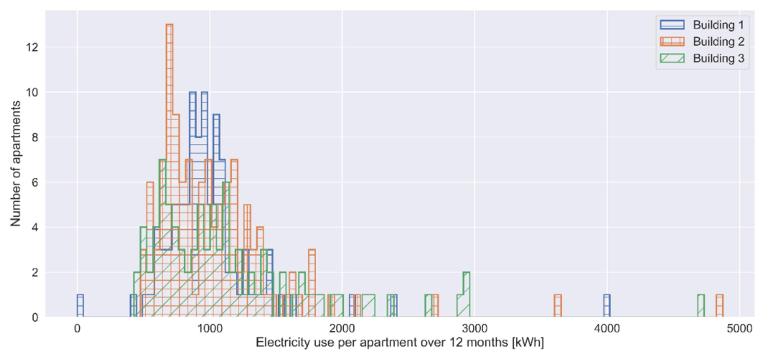
3.1.2. Electricity Use of Apartments

Figure 11 shows the monthly electricity use of all the 305 apartments in Testbed EM grouped by building. As expected, the electricity use in the months of June, July and August are lower than in other months, given that the users (students) are more likely to be away. Overall, the electricity use for each building is about 23.7, 27.2 and 28.7 kWh/m² and the total over 12 months is about 280 MWh. Figure 12 shows the daily electricity use in the apartments versus the average outdoor temperature. As qualitatively expected, the figure reveals a clear correlation with the outdoor temperature, especially considering the spring, winter and fall data.

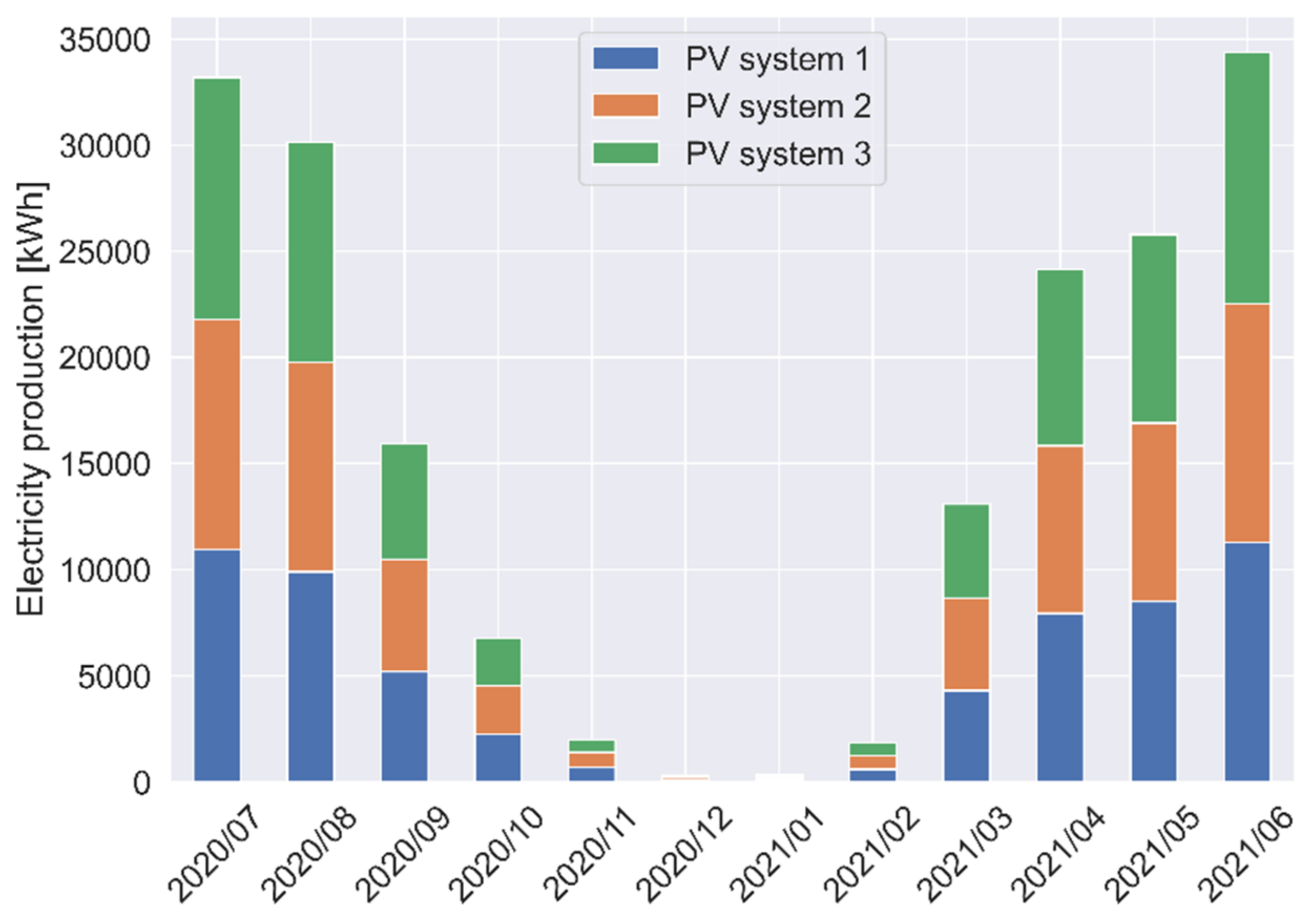
3.1.3. Electricity Production from PV Systems

The three PV systems installed include 667 PV, covering a total area of 1150 m². Figure 13 shows the monthly electricity production of the three PV systems. The total electricity produced over 12 months is about 188 MWh and the energy production per PV installation area is therefore about 163 kWh/m².

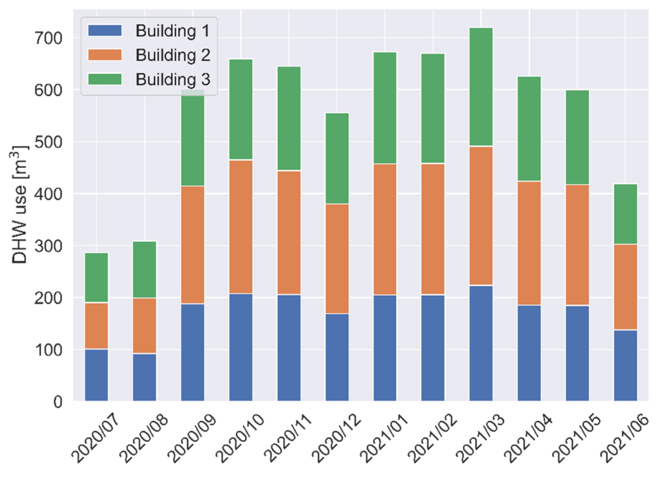
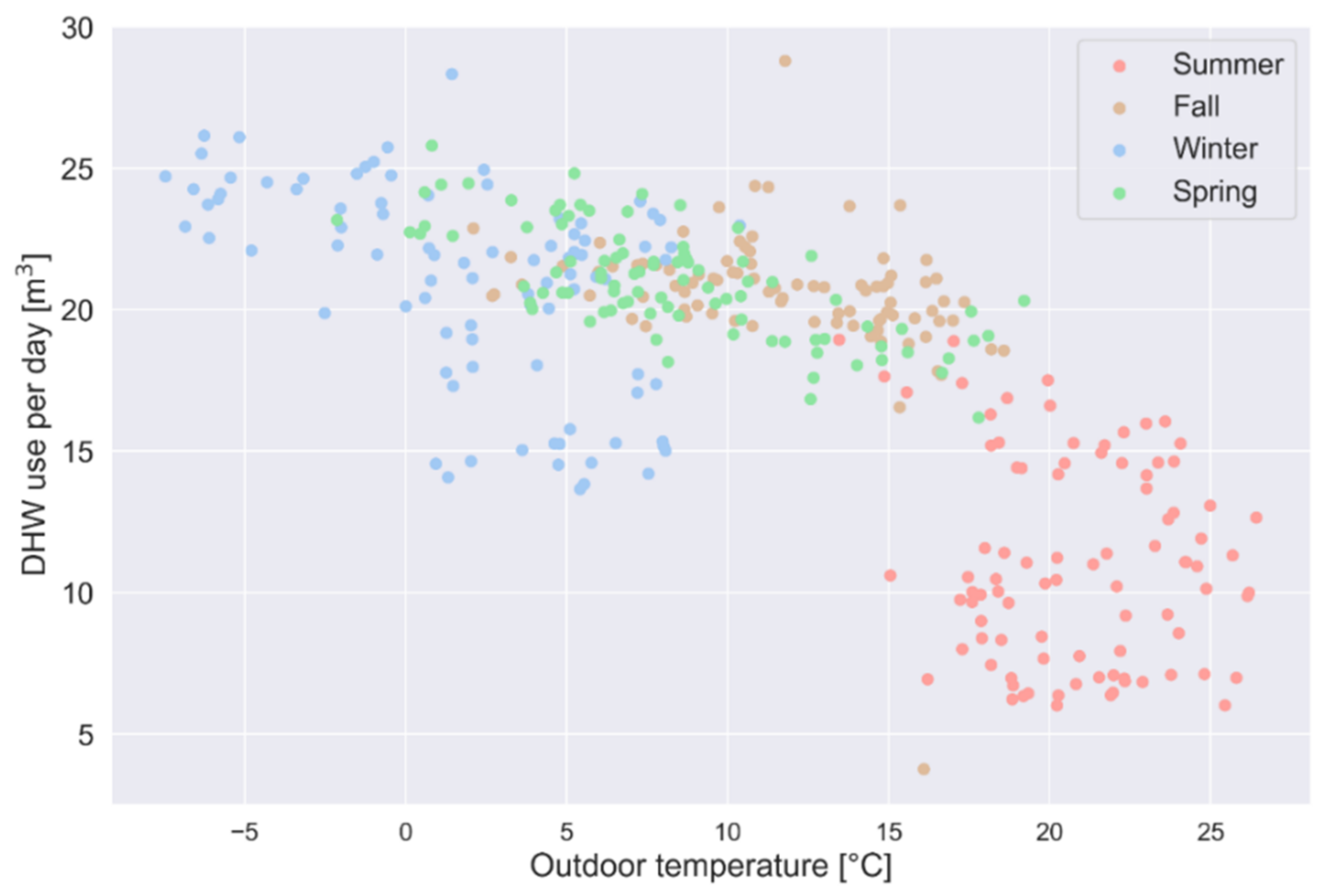
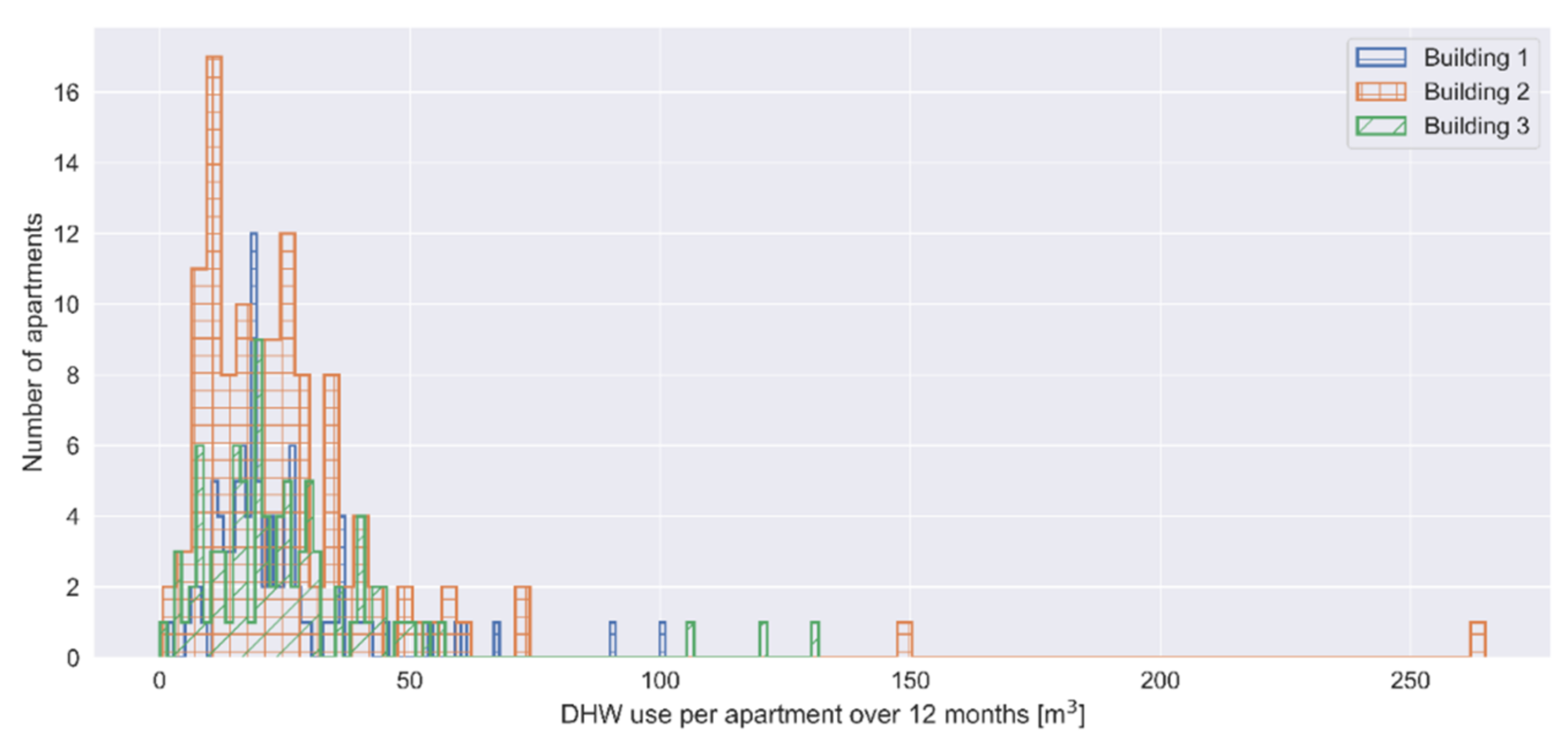
3.2. Domestic Hot Water (DHW)

Figure 14 shows the monthly DHW use from all 305 apartments. The total volume of DHW used over 12 months is about 6760 m³, equivalent to an average of about 22 m³ per year for each apartment, corresponding to about 60 L per day.

As expected, and as already observed for the electricity use, during the months of June, July and August the users (students) are more likely to be away. A contraction of the monthly consumption can also clearly be observed in December. The section dedicated to user behavior contains a more detailed analysis of the DHW use.

Similarly to the results proposed in Figure 10, Figure 12 and Figure 15 shows the daily use of DHW and reveals a slight correlation with the outdoor temperature.

3.3. Heat Pumps

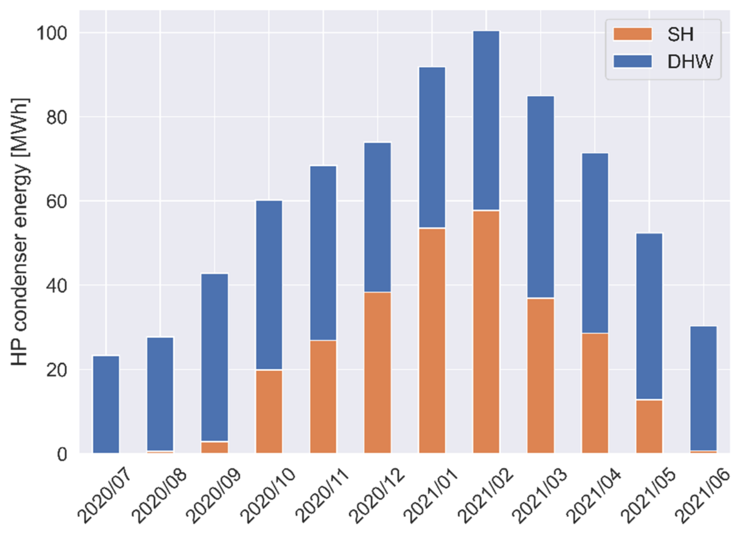
3.3.1. Heat Pumps: Delivered Energy

The heat pumps operate in two main operation modes: space heating (SH) and domestic hot water (DHW). Figure 16 shows the monthly energy production of the three heat pumps over the period analyzed. As qualitatively expected, the energy production in SH mode is higher during the winter months, with the peak in February, while the monthly energy delivered for DHW production is more uniform. Quantitatively, the energy delivered in SH and DHW mode over 12 months are about 279 MWh and 449 MWh, respectively, and the total energy is about 728 MWh, corresponding to a percentage ratio of approximately 60/30.

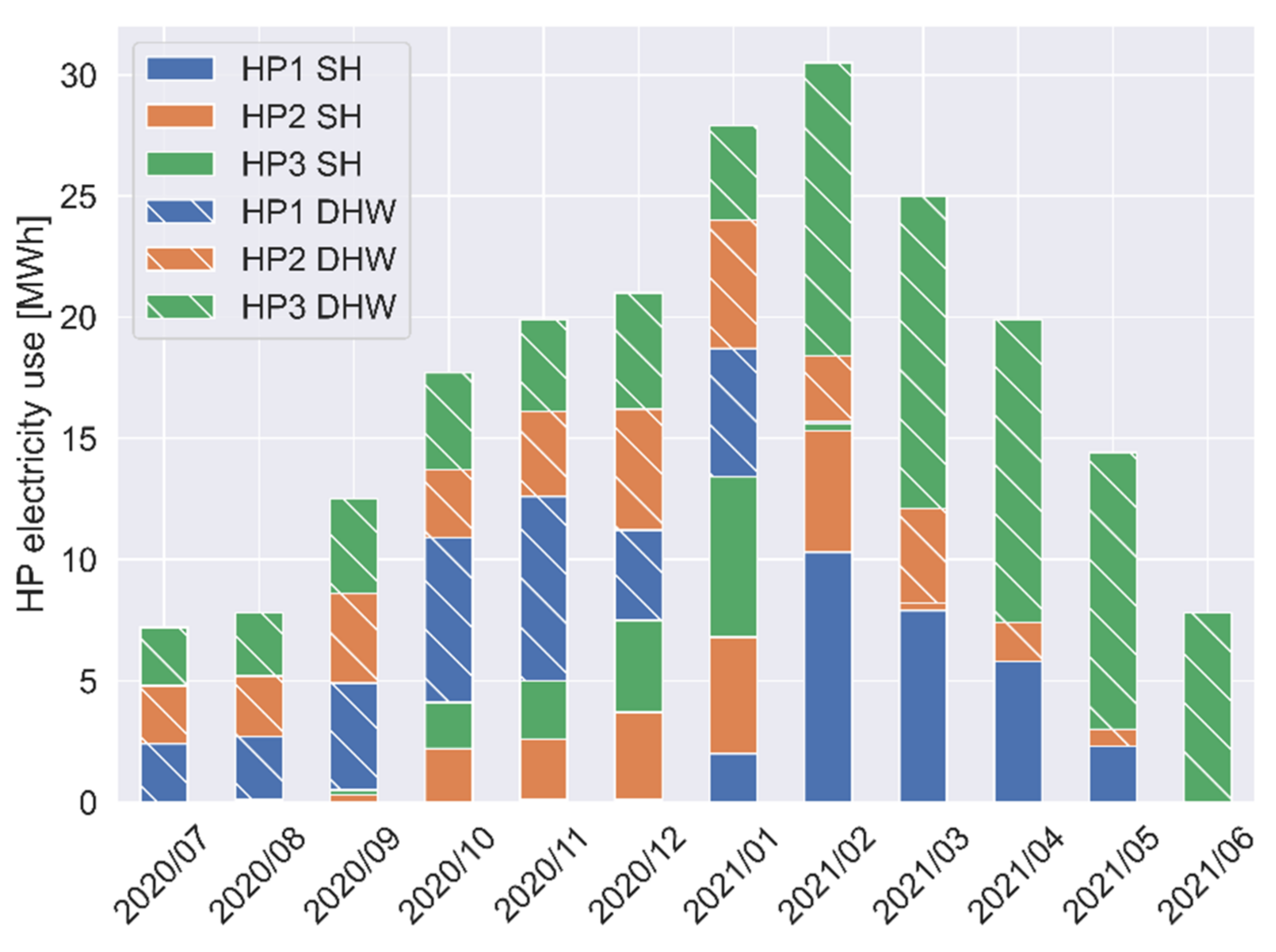
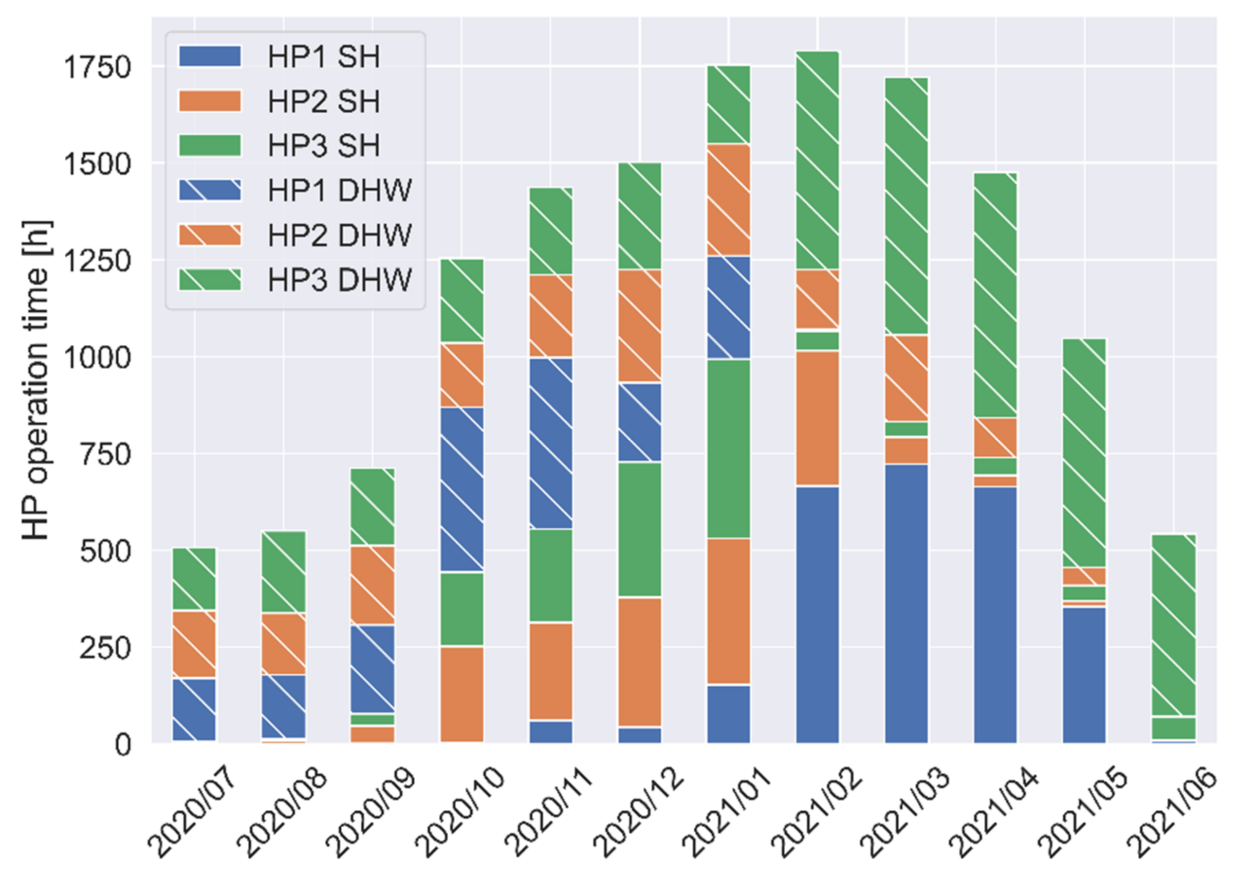
3.3.2. Heat Pumps: Electricity Use and Operation Time

Dedicated data points allow the heat pump units to be monitored in terms of electric power of the compressors, electricity use, operation mode and operation time.

Table 4. Heat pumps: monthly electricity use and operation time in SH and DHW modes.

	HP1				HP2				HP3
	SH		DHW		SH		DHW		SH		DHW
	MWh	h	MWh	h	MWh	h	MWh	h	MWh	h	MWh	h
2020-07	0.0	4.3	2.4	162.4	0.0	1.3	2.4	174.5	0.0	1.8	2.4	161.7
2020-08	0.0	0.1	2.6	166.0	0.1	7.8	2.5	160.1	0.0	4.1	2.6	212.0
2020-09	0.0	1.4	4.4	229.2	0.3	44.8	3.7	205.2	0.2	31.6	3.9	199.7
2020-10	0.0	3.3	6.8	426.1	2.2	248.3	2.8	165.3	1.9	191.7	4.0	219.2
2020-11	0.1	60.5	7.6	443.1	2.5	253.2	3.5	212.8	2.4	240.9	3.8	225.9
2020-12	0.1	43.3	3.7	204.2	3.6	334.7	5.0	292.1	3.8	350.0	4.8	276.9
2021-01	2.0	152.4	5.3	266.6	4.8	378.2	5.3	289.1	6.6	462.9	3.9	203.6
2021-02	10.3	665.7	0.1	5.0	5.0	349.6	2.7	153.4	0.3	51.0	12.1	565.0
2021-03	7.9	722.2	0.0	0.0	0.3	69.5	3.9	224.1	0.0	40.2	12.9	665.5
2021-04	5.8	664.1	0.0	0.0	0.0	28.5	1.6	102.4	0.0	46.4	12.5	634.3
2021-05	2.3	353.8	0.0	0.0	0.0	15.0	0.7	47.5	0.0	39.5	11.4	591.0
2021-06	0.0	9.2	0.0	0.0	0.0	0.8	0.0	3.7	0.0	58.2	7.8	470.3
Total	29	2680	33	1903	19	1732	34	2030	15	1518	82	4425

shows the monthly aggregated values used to build Figure 17 and Figure 18. In terms of operation time, HP3 operated about 35% more than HP2 and about 23% more than HP1. Although the details of the control and operation strategies are not available, the inspection of the operation modes reveals also that the three heat pumps operate following non uniform patterns. For instance, HP1 was used almost exclusively in DHW mode during the 6 months of 2020 and almost exclusively in SH mode during the six months of 2021. Overall, HP3 operated in DHW 60% more than HP1 and about 76% less in SH mode. It is unclear whether the observed operation patterns follow a dedicated design choice or represent the side effects of the implemented control algorithm. However, the unbalanced operation time and modes between the three units can potentially lead to maintenance issues and should be actively monitored.

3.3.3. Heat Pump System: Performance

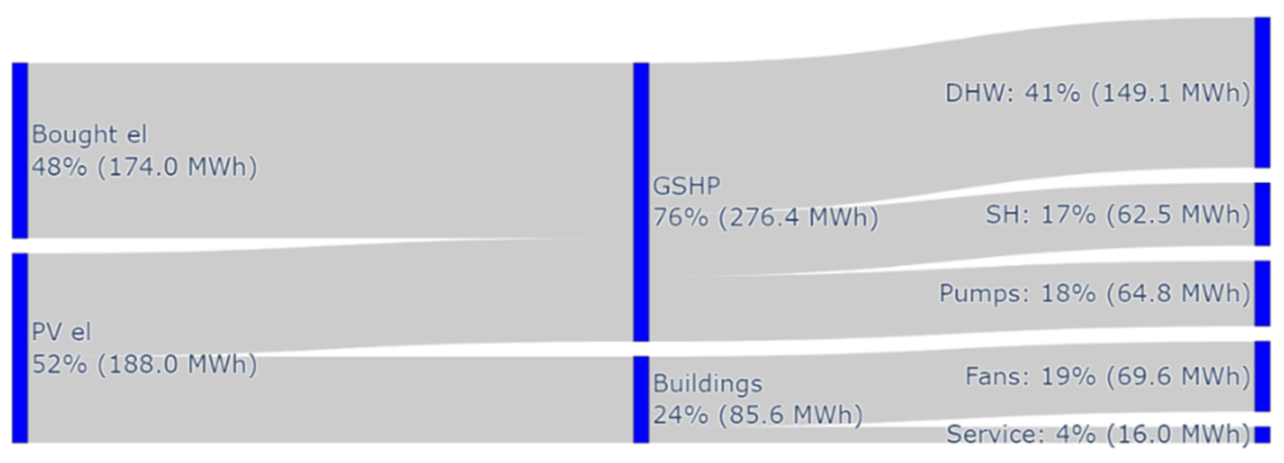
The monitoring system includes a dedicated data point providing the aggregated condenser energy of the three heat pumps, but the condenser energy of the individual heat pump unity is unfortunately not available.

In order to provide an overview of the heat pump system performance, this analysis include the results of the calculation of average COP, evaluated considering the overall energy provided at the condenser level and the electricity use of the compressors. The results aggregated by month are provided in

Table 5. Heat pump system: average COP.

Month	COP Avg	COP * Avg	Mode Ratio ** [%]
2020-07	3.2	2.1	98
2020-08	3.5	2.5	97
2020-09	3.4	2.7	89
2020-10	3.3	2.7	64
2020-11	3.3	2.7	61
2020-12	3.3	2.6	51
2021-01	3.2	2.6	43
2021-02	3.2	2.7	40
2021-03	3.3	2.8	51
2021-04	3.5	2.8	49
2021-05	3.5	2.6	61
2021-06	3.6	2.4	87

* Including GSHP circulation pumps. ** Mode ratio: operation time in DHW mode vs. total operation time.

. Overall, the average COP over 12 months of operation is about 3.4. In order to evaluate the performance of the GSHP system it is important to include the electricity use of the circulation pumps in the evaluation of the COP. As shown in the table, the monthly average of the COP evaluated considering the circulation pumps is between 2.1 and 2.8, with an overall average of about 2.6.

Table 5 includes also the monthly percentage of the operation mode ratio, defined as the hours during which the heat pumps operated in DHW mode over the total operation time. A mode ratio of 100% would indicate that the heat pumps operated only in DHW mode. Although the maximum value of the mode ratio corresponds to the minimum value of the COP, as qualitatively expected, the COP values for low mode ratio are not always consistent. Further investigations including temperatures and secondary fluid flows on both the evaporator and condenser sides could clarify these inconsistencies but have not been carried out in this study.

3.4. Energy Flows

Considering the analyzed period of 12 months, between July 2020 and June 2021, the Sankey diagram in Figure 19 shows the energy flows of the system based only on electricity use.

The values displayed lead to a few considerations. Total energy use from the facility is about 687 MWh per year. Considering that the total heated area of 10,590 m² the value corresponds to an annual energy use of 65 kWh/m². The energy value under the slot “service” accounts for the electricity use of the servers, the control system and a water pressurizer pump. The slot named “fans” includes the electricity used by the ventilation system.

The electricity use of the geothermal heat pump system is about 276 MWh, corresponding to an annual energy use of about 26 kWh/m². Considering the electricity for space heating (SH) and domestic hot water production (DHW), the DHW part is 70% of the total. Notably, the electricity use of the circulation pumps is almost the same (even slightly higher for the analyzed period) as the heat pump electricity required for heating the apartments. This helps to show that the circulation pumps are a relevant and fundamental part of a GSHP system and that they need to be included in the evaluation of the system performance. Additionally, this aspect will play a more and more relevant role as the overall performance of the buildings improve. It is also worth noticing that the energy used by the ventilation system (about 69 MWh) is comparable in value with the geothermal circulation pumps and energy for space heating.

Notably, Figure 19 maps the energy flows of the buildings considering only the electricity used for space heating, domestic hot water and ventilation. The electricity use of the apartments and the laundry are therefore excluded from the calculations. The total bought electricity is 174 MWh per year, which is 7% lower than the energy produced by the PV systems. In this scheme, the total energy use by testbed EM is about 362 MWh per year, corresponding to an annual energy use of 34 kWh/m². It is important to notice that the energy flows displayed in Figure 19 represent the net energy flows over 12 months and do not specify the portion of produced electricity that is actually self-consumed and the part that is sold back to the grid. The exact quota of electricity that is self-consumed over the 12 months analyzed is currently not available. Overall, 76% of the total energy is used by the geothermal system. The energy for domestic hot water production is 41% of the total while the ventilation system, the circulation pumps and the energy for space heating account each for about 18% of the total.

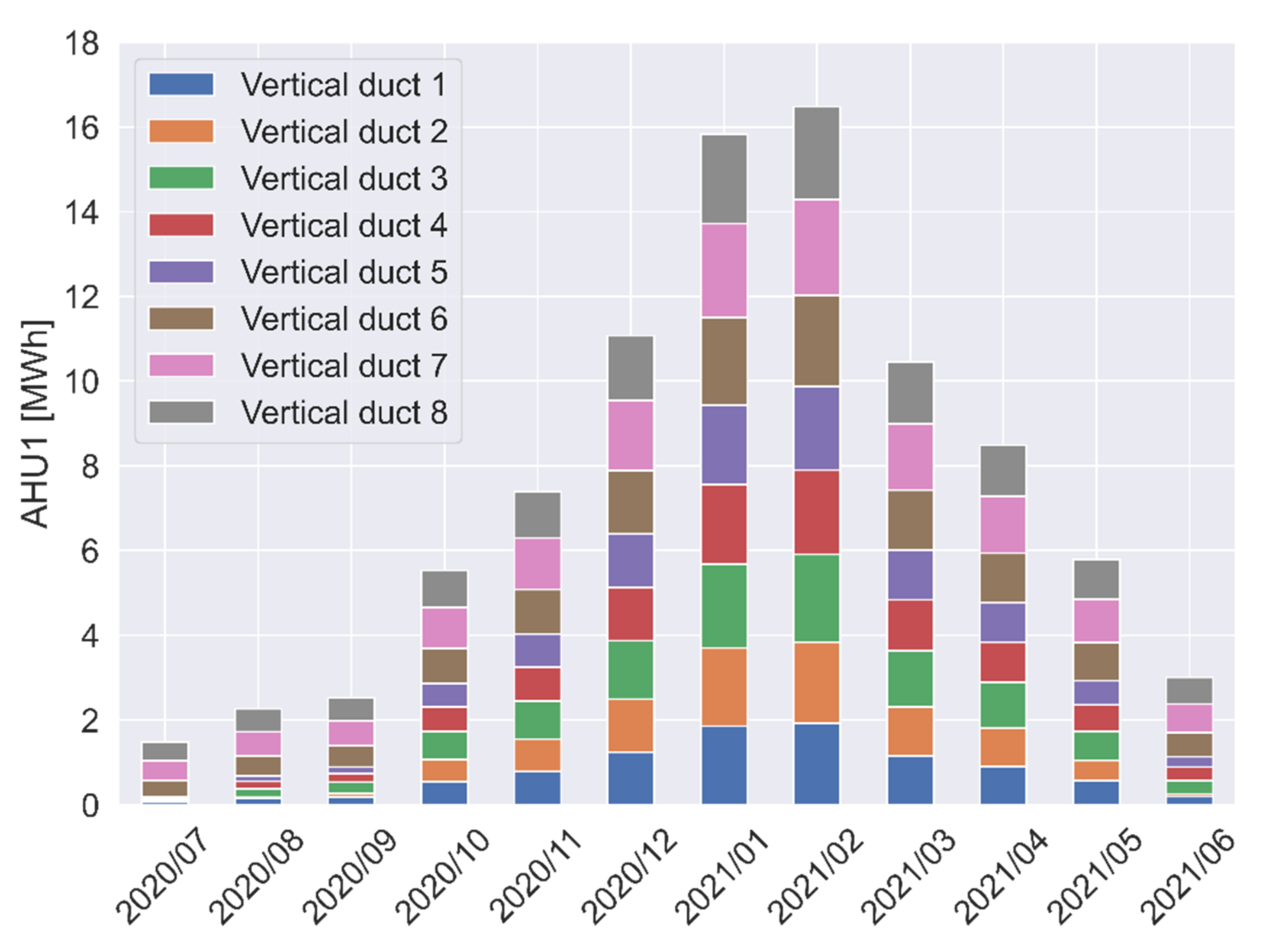
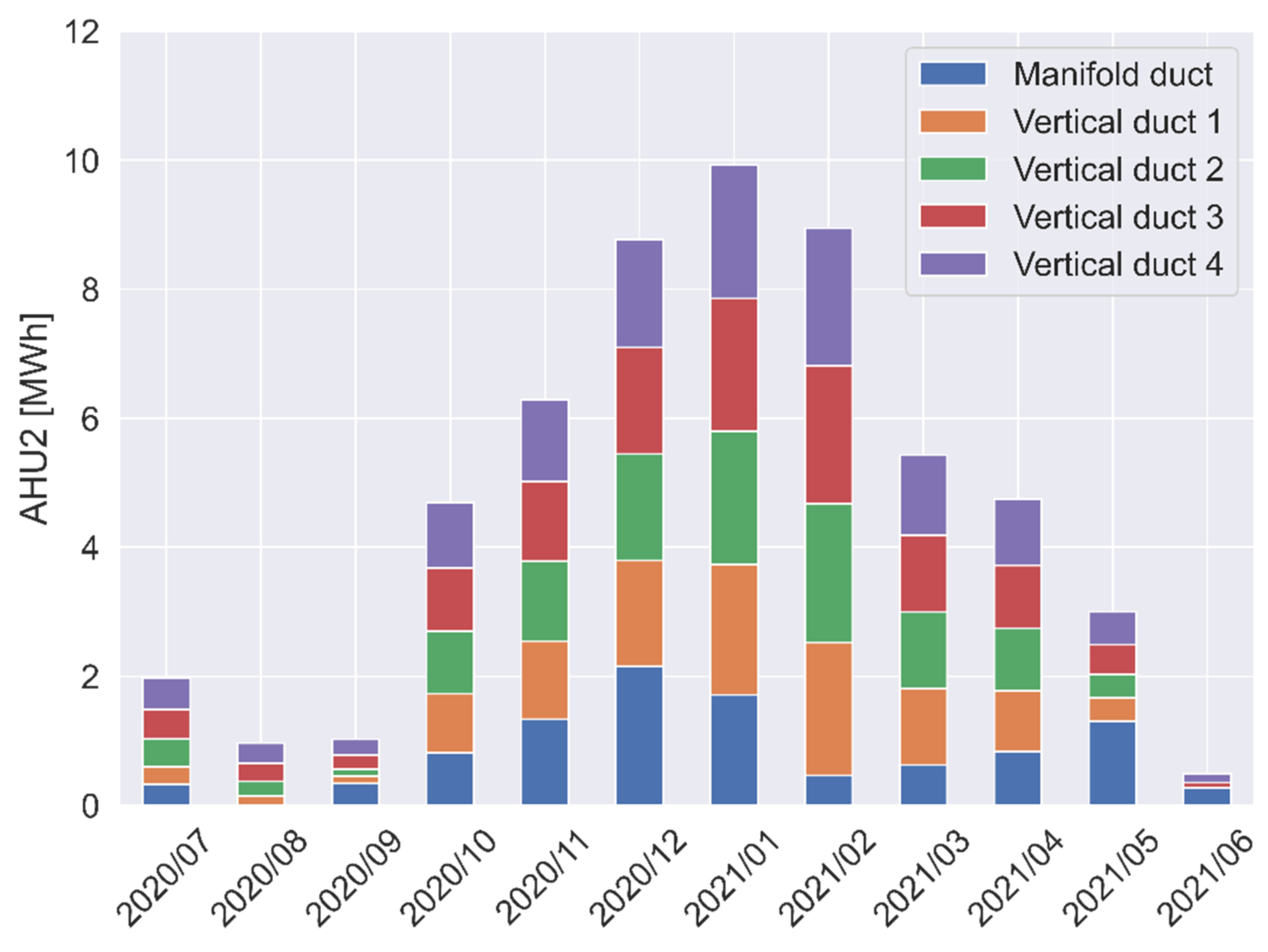
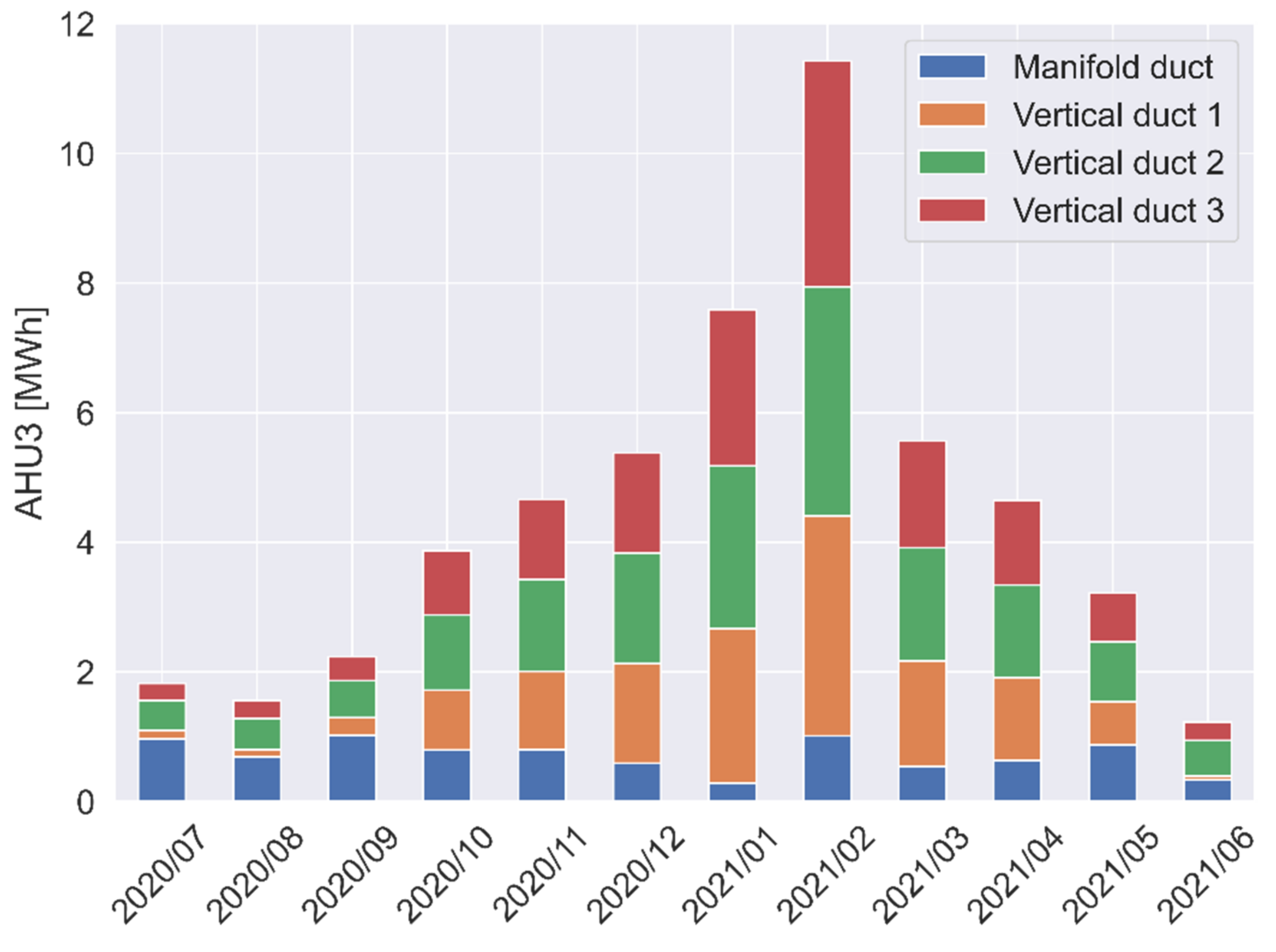
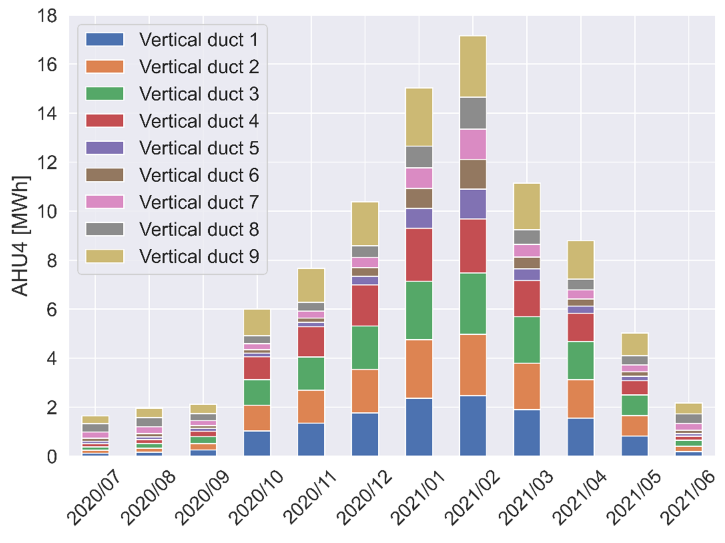
3.5. Air Handling Units (AHUs)

The analysis of the four AHUs available in the system included the calculation of the energy delivered to the apartments using the data logged in the monitoring system. Figure 20 shows the simplified schematic of the supply air flow including an overview of the data points used in the calculations. For each AHU, the heating rate ${\dot{Q}}_{AHU}$ is calculated as shown in Equation (3).

$${\dot{Q}}_{AHU}=\dot{m}\times c\times \left[\left(T_1-T_0\right)+{\displaystyle \sum }_{k=1}^N\frac{1}{N}\times \left(T_{k1}-T_1\right)\right]$$

(3)

where c is the air specific heat (assumed to be constant at 1.003 kJ/kg/K), $\dot{m}$ is the air mass flow rate and T_k1 is the temperature measured after the heating coil of “vertical duct k”. Notably, the evaluation of the volume flow rate was adjusted considering the air density as a function of the air temperature. As specified before, the number of vertical ducts available on the supply side of the 4 AHUs installed in Testbed EM is different for each AHU (see Figure 5). Additionally, an additional “heating coil 0” is installed in the manifold duct of AHU2 and AHU3 (see Figure 20). At each vertical duct the flow is controlled through duct valves. Although the opening of the valves is monitored by means of dedicated data points, the logged data was considered unreliable in this study and therefore not used in the calculation. Instead, the supply air flow is assumed to be equally distributed between in each of the N heating levels.

The results of the calculations are shown in the following Figures (Figure 21, Figure 22, Figure 23 and Figure 24). Overall, the energy delivered through the ventilation system over 12 months is about 112 MWh for Building 2 (AHU2 and AHU3) and about 92 MWh for Building 1 and Building 3.

It is important to notice that relevant “free heating” contributions can be identified in May, June, July, August and September. As shown in Figure 25, in those months the heat delivered through the ventilation system to the apartments appears to be higher than the part of the heat that the heat pumps generated in space heating mode (SH). Although this contradictory and unexpected result has been investigated the possible explanations are not conclusive. One possible reason of the identified inconsistencies may be related to a poor insulation of the ventilation ducts. The practical consequence of this issue is the delivery of heat to the apartments when there is no heat demand. For this reason, it is important to notice that a periodic (if not continuous) supervision of the monitored data is critical for the identification of faults or performance degradation in the system. To this regards, automated solutions could also be adopted but are not currently implemented in this system.

Considering the winter months of December, January and February, the difference between the energy generated by the heat pumps in SH mode and the heat delivered by ventilation is about 3 MWh per month. This result can be considered as a preliminary estimation of energy loss of the heating distribution system.

3.6. Indoor Environmental Quality: Assessment of Indoor Air Quality and Thermal Conditions

The indoor temperature and CO₂ concentration of all the apartments have been analyzed in order to evaluate the comfort indoor condition. As already mentioned in Section 2.2.2, other measurements fundamental for a thorough assessment of comfort, such as the relative humidity, are unfortunately not currently available in Testbed EM.

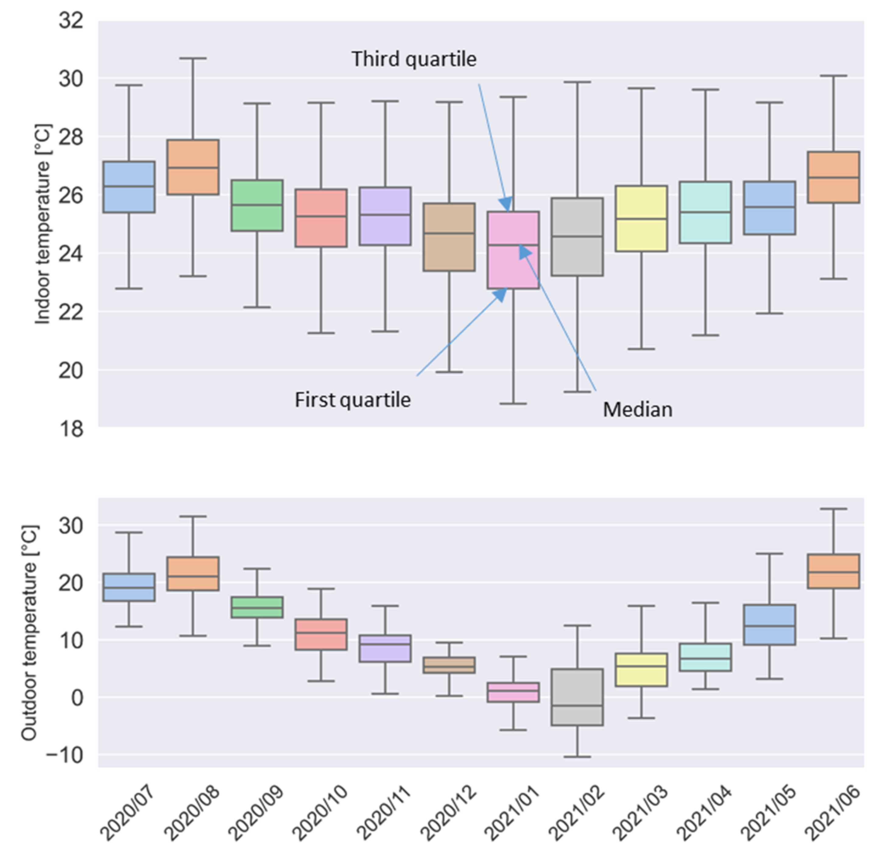
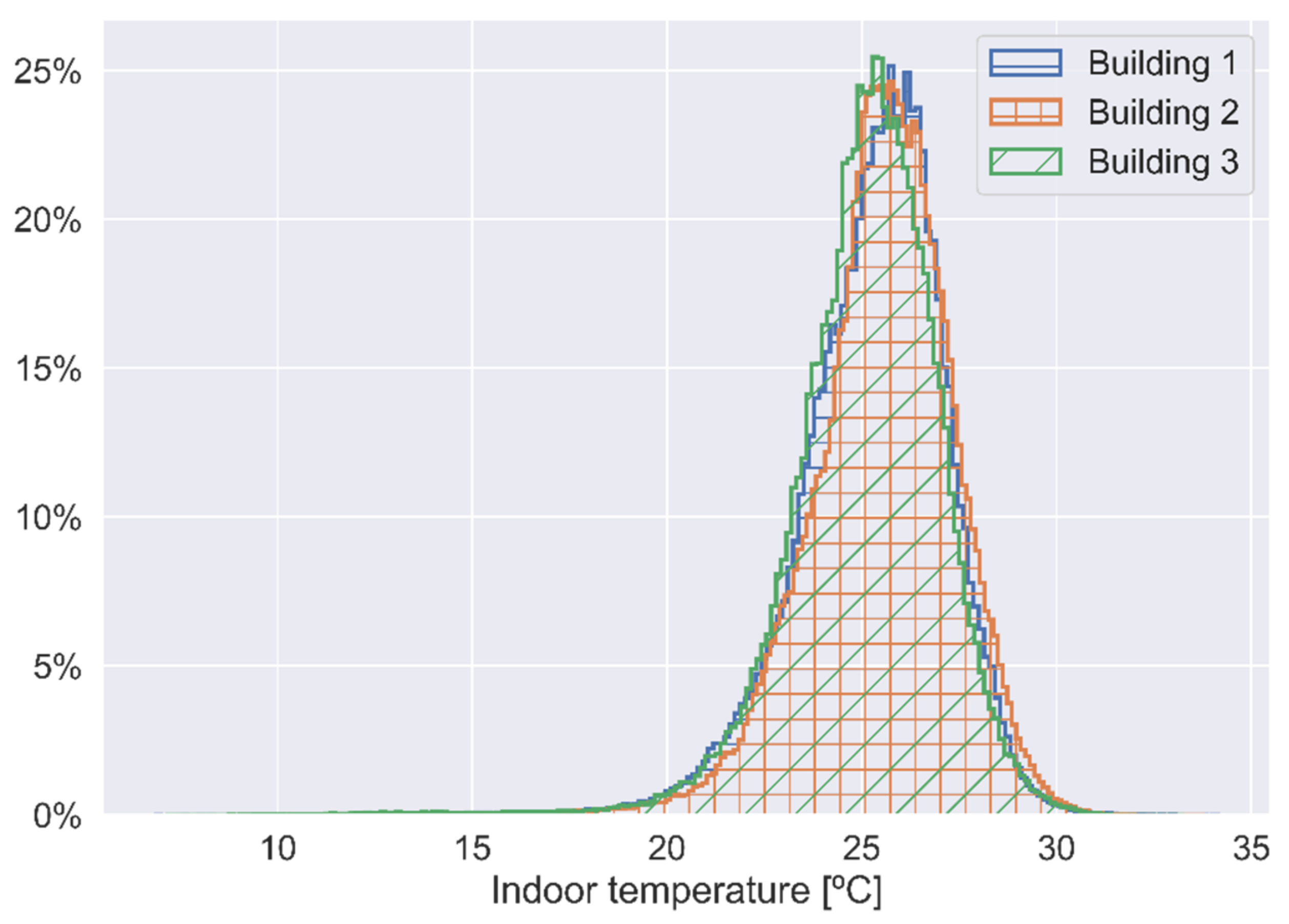
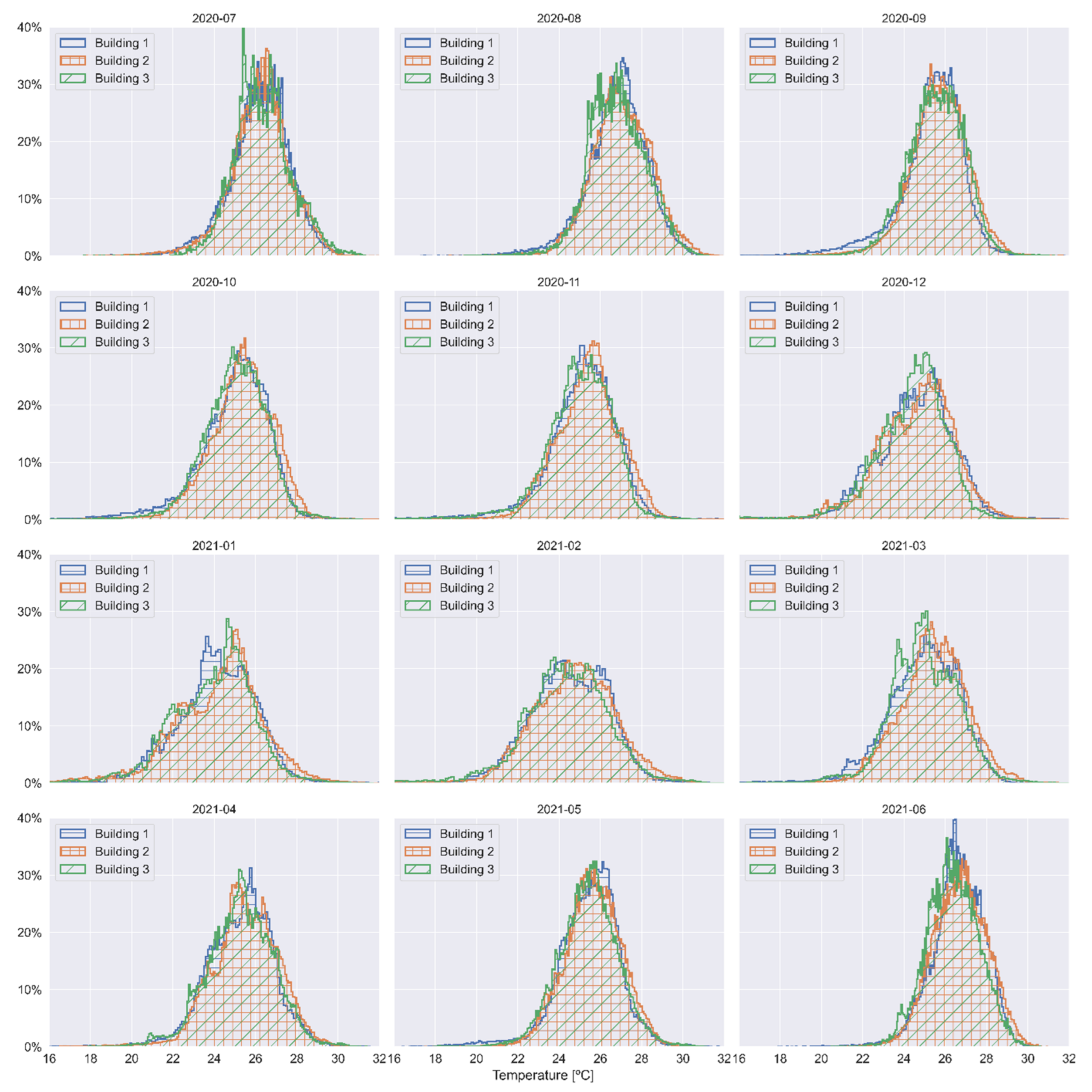
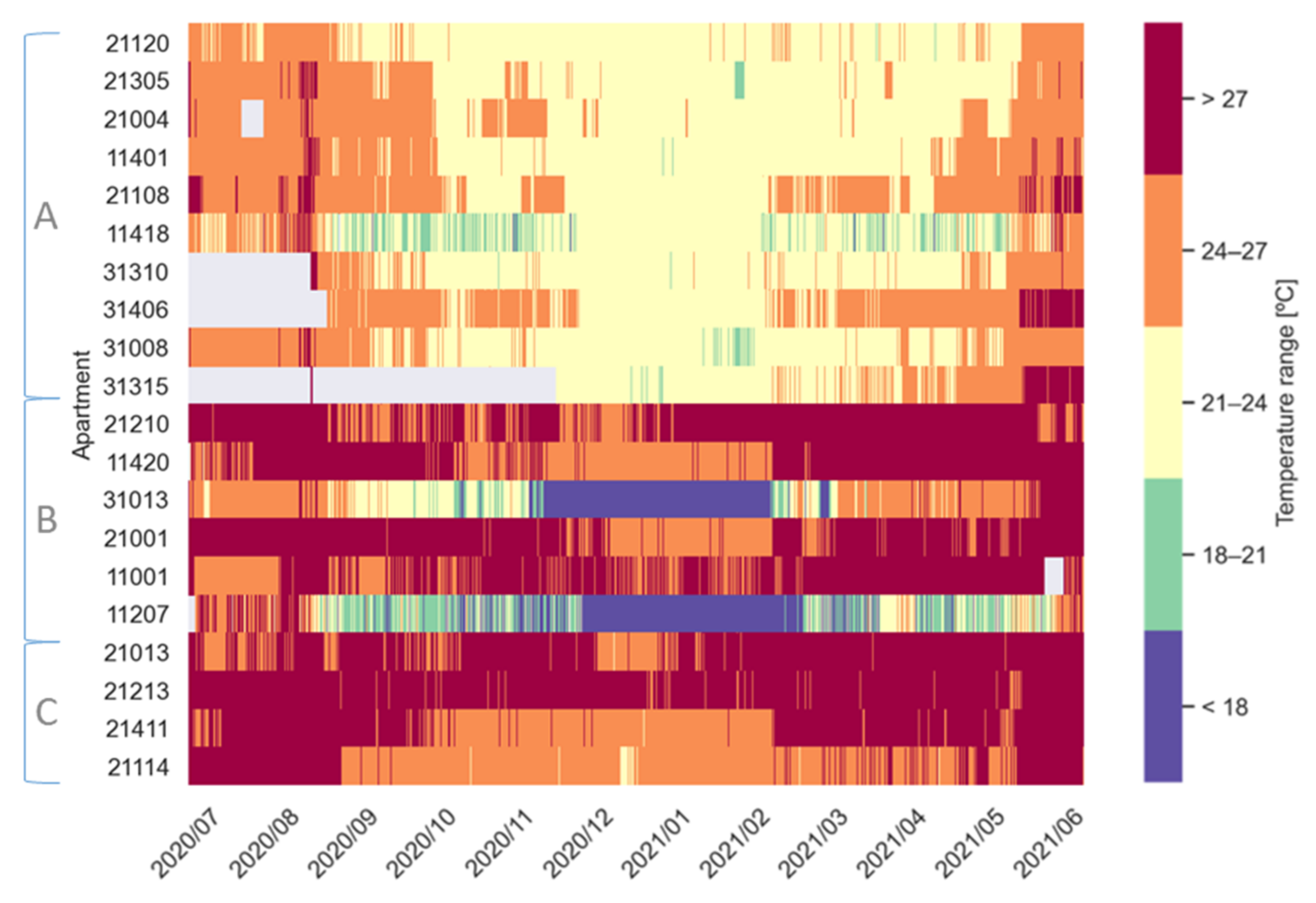
3.6.1. Indoor Temperature: Overview

Qualitatively, over the 12 months of data included in this study the values of indoor temperature in the apartments presents a large variability and a relatively high average. Figure 26 shows median, upper and lower percentile temperature distributions per month while Figure 27 shows the temperature distribution considering all the hourly values available from the three buildings. During the period between October and April the median temperature in the apartments is always above 24 degrees, which is higher than the indoor temperature between 20 and 24 °C recommended by the Swedish National Board of Health and Welfare [30], highlighting a potential for reducing the energy demand. Figure 28 displays more in detail the distribution of the temperatures in the apartments in the three buildings. During the warmer months—July, August 2020 and June 2021—the median temperature in the apartments is above 26 degrees, suggesting an overheating issues in the apartments. In general, no significant deviation between the buildings can be observed.

The hourly indoor temperature of all apartments has been parsed in order to identify recurrent conditions and possible patterns. For the sake of brevity, the results of the analysis are here reported with the support of a limited number of examples. Figure 29 provides an overview of the indoor temperatures in a subset of apartments selected and grouped based on arbitrary temperature ranges varying from below 18 °C to above 27 °C. The figure includes the heat map chart built considering the hourly values over the 12 months of data available. The apartments included in the figure are intentionally grouped and sorted to focus on a few relevant considerations.

The results can be simplified into three main patterns. A first group of apartments (group A in the figure) presents temperatures within qualitative comfortable ranges (21–24 °C) in the coldest months and only with moderate overheating during the warmest months. A second group of apartments (group B) shows low temperatures in the coldest months and overheating in summertime. Finally, a third group of apartments (group C) shows consistent overheating during the coldest months and extreme overheating during the warmest months.

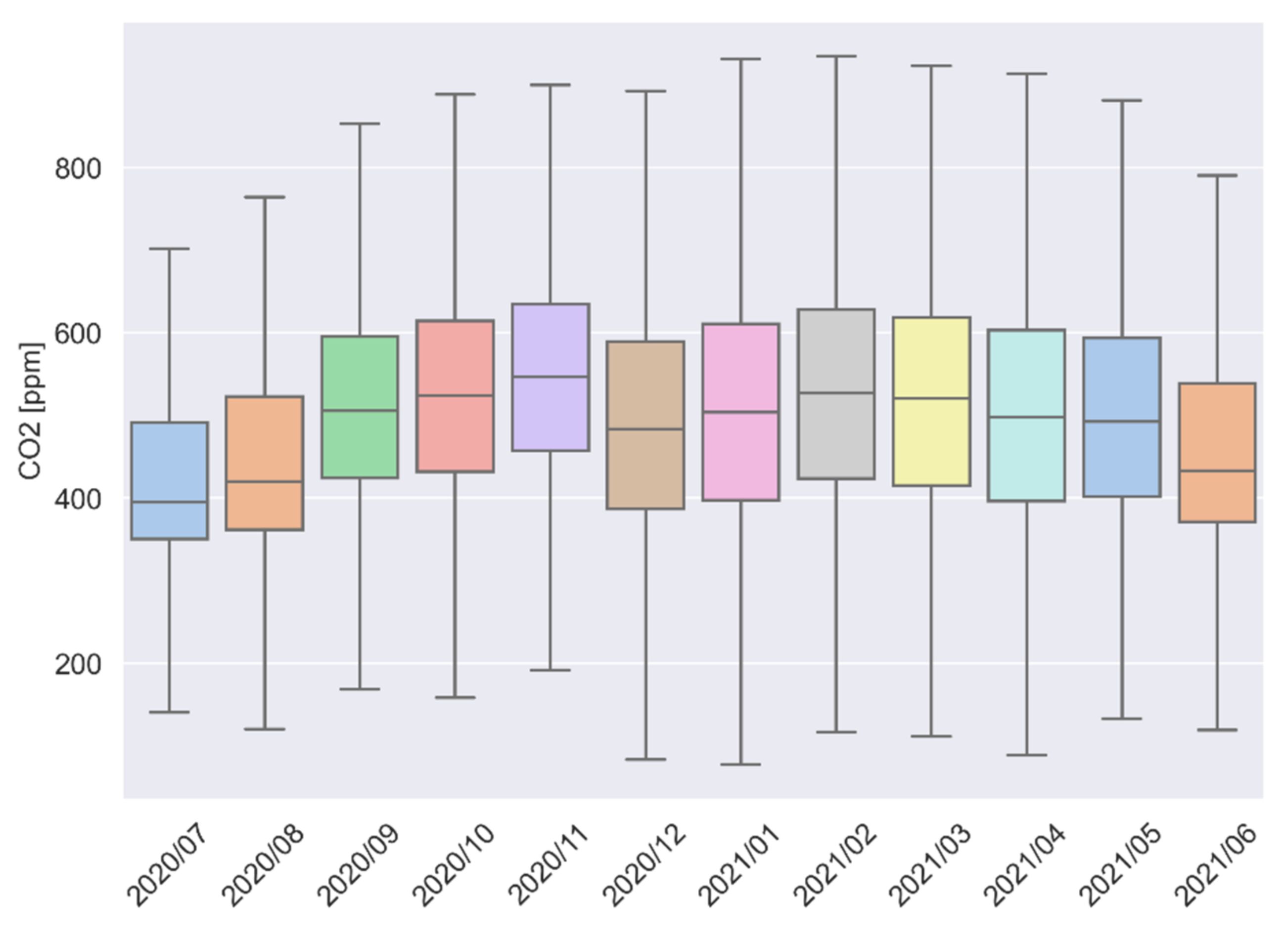
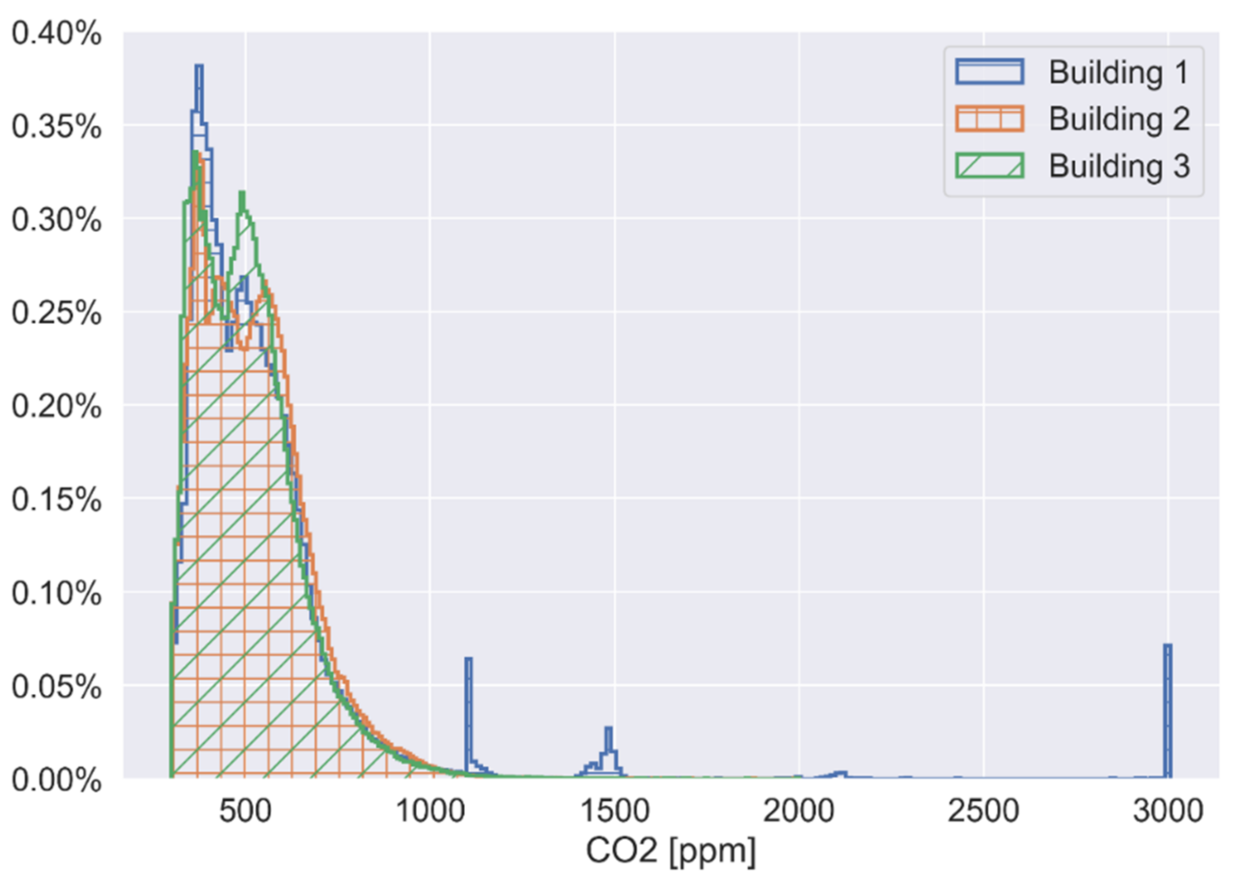
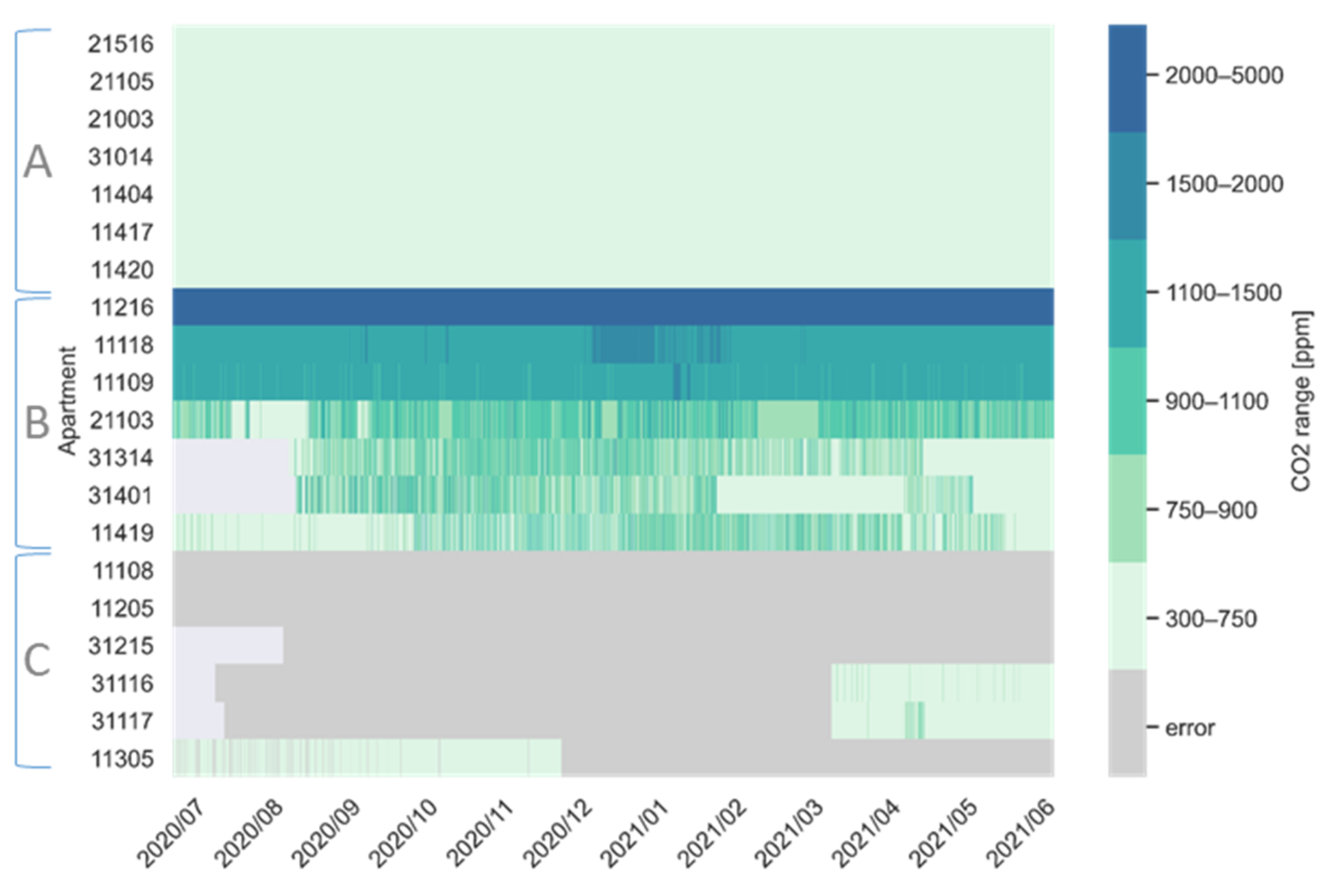
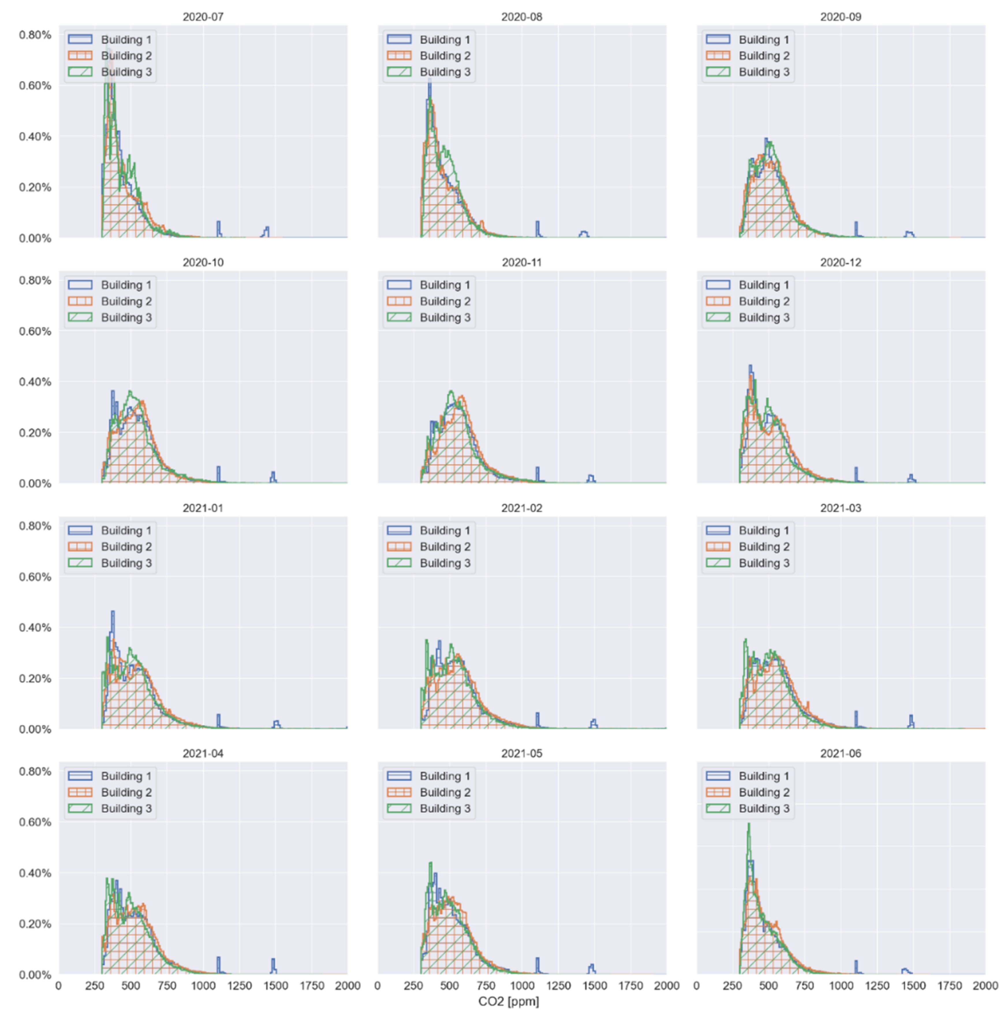
3.6.2. Overview on Indoor Air Quality: CO₂ Concentration

The considerations on the air quality in the apartments in the buildings are based on the CO₂ concentration measurements. Figure 30 summarizes the monthly distribution of the CO₂ concentration in the apartments. The median monthly values are between 400 and 600 ppm and the distribution maximums are below 1000 ppm, with highest values in January and February 2021. Although the outliers are not included in the figure, the bar whiskers show minimum values below 200 ppm that suggest the presence of measurements errors. Figure 31 shows the probability density of the CO₂ concentration in the 3 buildings over 12 months, confirming that, approximately, the values are typically in the range 400–600 ppm.

Similarly to Figure 29 for the indoor temperature values, Figure 32 provides an overview of the CO₂ concentration in a subset of apartments selected and grouped based on arbitrary ranges. In particular, from top to bottom, a first group (group A) includes apartments where the hourly CO₂ concentration values are always in the range 300–750 ppm. A second group of apartments (group B) shows hourly peaks of CO₂; within this group, it should be noted that the persistent high values of apartments 11216, 11118 and 11109 suggest possible malfunctions of the sensors that could not be verified in this study. A third group (group C) of apartments presenting clear signs of sensor malfunctions is also included in the figure. Notably, in this figure, all hourly values below 300 and above 5000 fall into the “error” range.

Figure 33 shows the details of the CO₂ values distribution for each month.

3.7. User Behavior

Occupants’ behavioral patterns are known to affect the energy performance of buildings. Based on the results of the analysis overview, a few examples have been selected to further investigate the details and possible reasons of anomalies.

The evidence collected in this paragraph illustrates primarily examples of the detectable impact of building occupants on the indoor environment and includes an overview of the resources directly controllable by building occupants (DHW and dwelling electricity).

3.7.1. Controllable Resources: Consumption of Dwelling Electricity and Domestic Hot Water

The analysis of the data of the indoor temperature and the CO₂ concentration presented in the previous sections has been combined with a detailed parsing of the electricity and DHW use only briefly summarized in Figure 34 and Figure 35, aiming at explaining unexpected or extreme values and identifying possible user patterns.

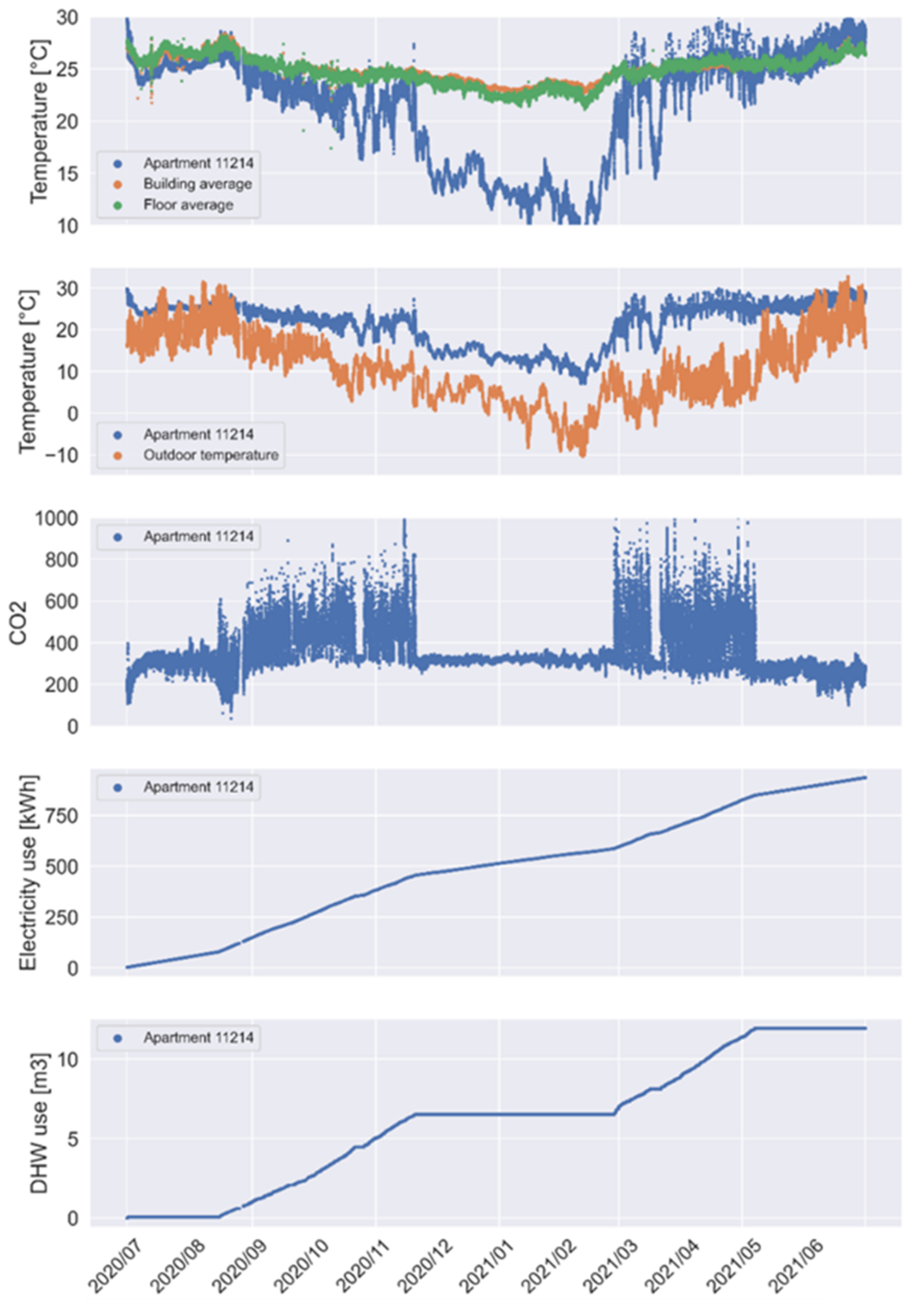
3.7.2. Indoor Comfort and User Behavior: Study Case 1

A case study considers apartment number 11214 (see Figure 36), where the time series indoor temperature, the CO₂ concentration, the DHW use and the electricity use from one apartment are plotted over 12 months, as shown in Figure 37. More in details, the indoor temperature is first shown together with the average indoor temperature of the apartments in the same floor (floor 1) and the average indoor temperature from all the apartments of the same building (Building 1). Moreover, the indoor temperature is also included in a second subplot together with the outdoor temperature. More in details, the indoor temperature is first shown together with the average indoor temperature of the apartments in the same floor (floor 1) and the average indoor temperature from all the apartments of the same building (Building 1). Moreover, the indoor temperature is also included in a second subplot together with the outdoor temperature.

Apartment 11214 was selected for a deeper analysis due to the unexpected low temperature recorded for a relatively long period. The inspection of the figure reveals in fact that for more than three months (from end of November 2020 until March 2021) the indoor temperature recorded was about 15 °C or lower. Additionally, in the same period, the indoor temperature evolution follows quite well the outdoor temperature values. The middle subplot of Figure 37 shows the CO₂ concentration in the apartment, clearly showing that in the three months where the indoor temperature was unexpectedly low, the CO₂ concentration was almost perfectly stable at a value of about 380 ppm. Although a clear confirmation is not available, these observations indicate that the low indoor temperature is likely due to the fact that the tenant left the apartment for about three months leaving the window open, or not completely close. Additional confirmations of this hypothesis are given by the cumulative DHW use and electricity use. The DHW use is in fact zero over the three months of absence of the tenant and the electricity use present a clear change of trend.

This selected example brings to a few considerations. The type and amount of sensors installed in the apartments allow both quite a useful overview of the indoor air quality and clear identifications of some anomalies. Inferring the long absence of the tenant while the windows in the apartment were left not completely closed was in fact possible just by inspecting the temperature and CO₂ profiles. The data from electricity and DHW meters were useful to confirm the explanation of the anomaly. Although the energy waste due the anomaly here described was not quantified in this study, it is clear that such user behaviors have an impact to the building energy use. Nevertheless, data available is currently not continuously used for the identification of such anomalies and there is currently no control or alarms available in the buildings to track or prevent this type of situations.

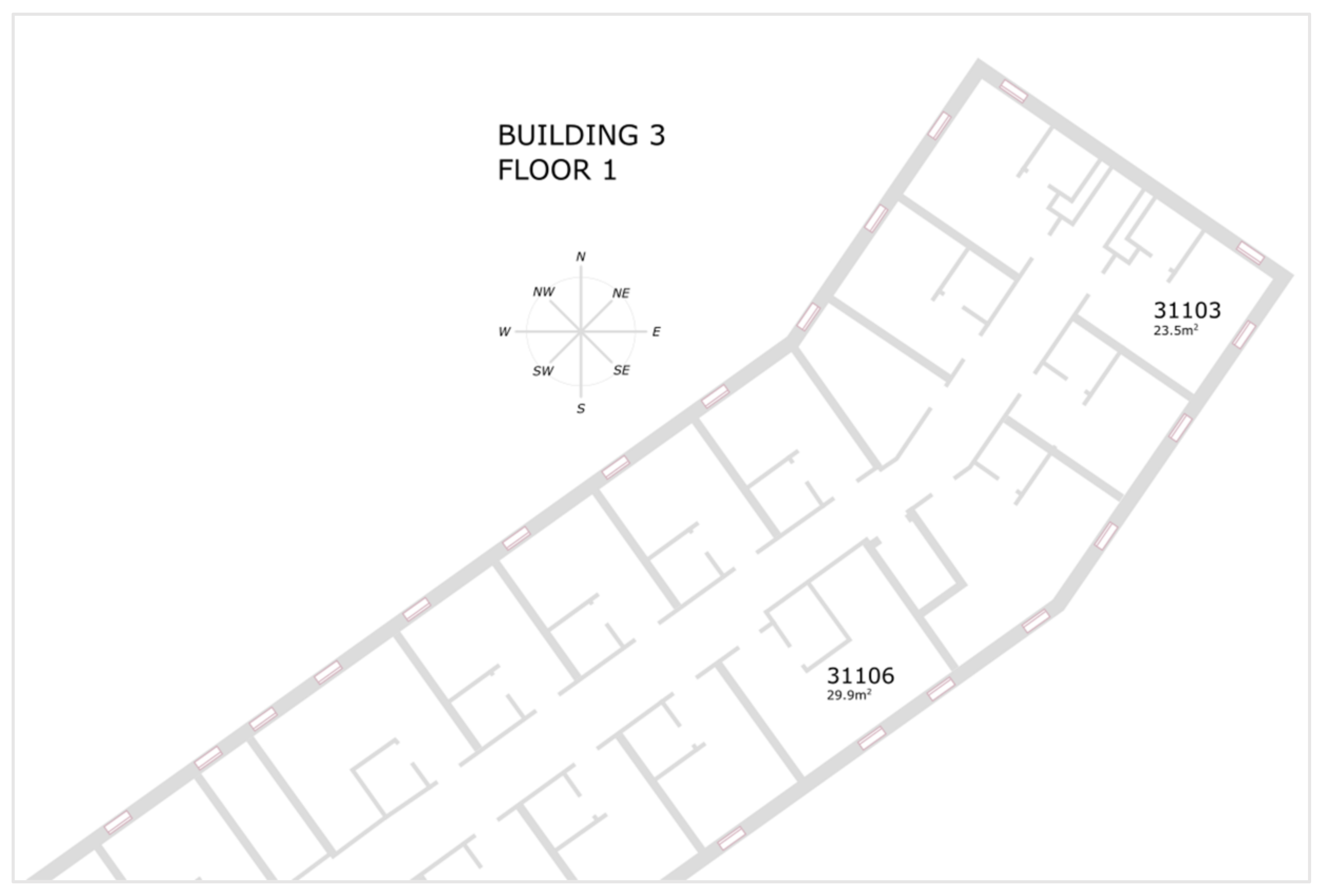
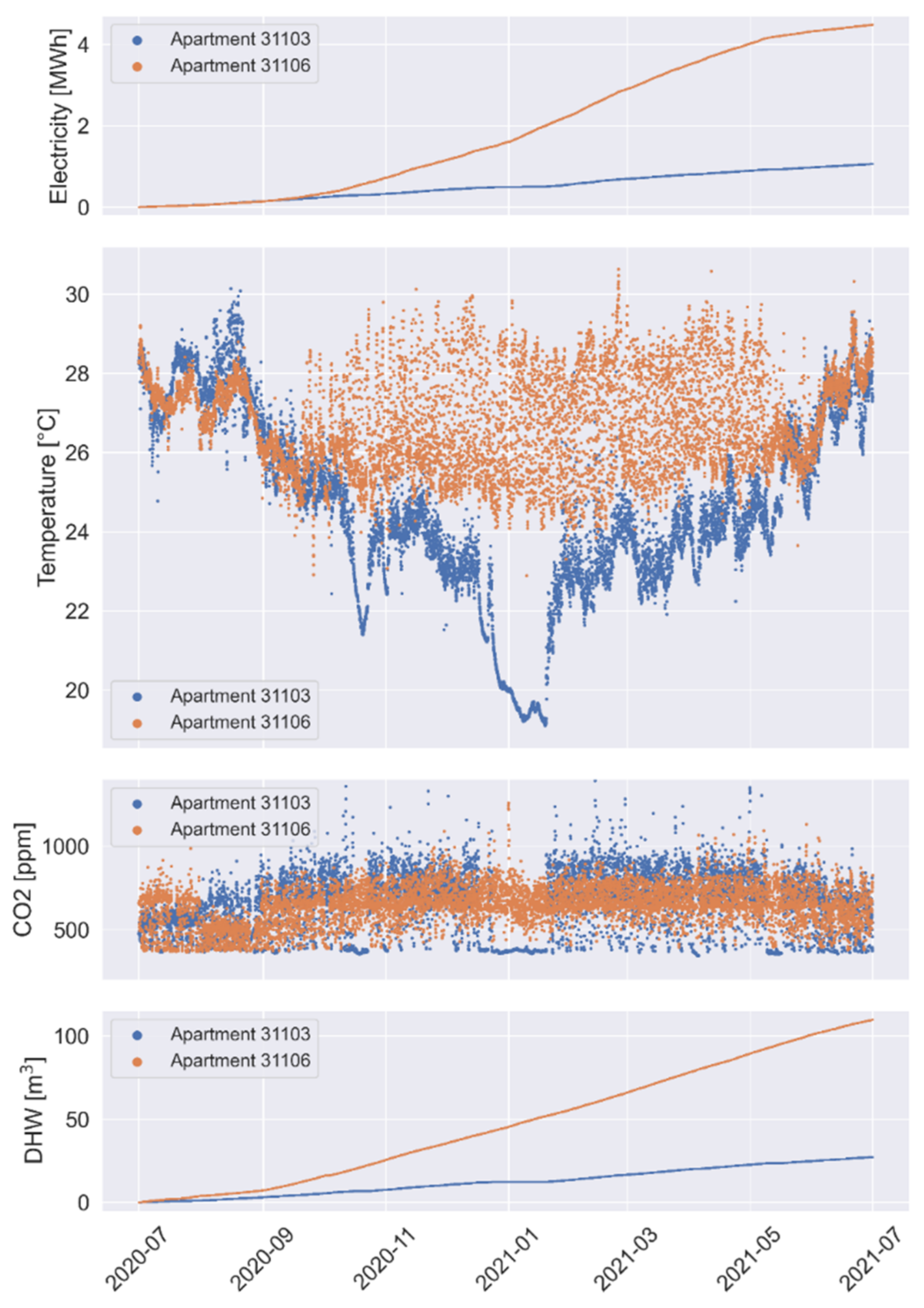
3.7.3. Indoor Comfort and User Behavior: Study Case 2

A second example proposed in this study involves the comparison of measurements from two apartments located on the same floor of Building 3, as shown in Figure 38. The two apartments have been selected with the intention to identify different behavioral patterns in similar conditions. Figure 39 shows, from top to bottom, electricity use, indoor temperature, CO₂ concentration and DHW use of apartments 31103 and 31106, located on the first floor of Building 3 and having an area of 23.5 and 29.9 m², respectively. Both apartments are located on the same side of the corridor facing south-east. More in details, apartment 31103 is located on the corner of the building and has one window on the north-east wall and one windows on the south-east wall, while apartment 31106 has two windows facing south-east. The inspection of the subplots of Figure 39 clearly reveals different indoor temperature patterns and different trends of electricity and DHW use. In particular, in the periods July–September 2020 and May–June 2021, the indoor temperature measurements show approximately the same evolution and from the CO₂ measurements both apartments seem to be in use. In contrast, in the period between October 2020 and April 2021 the indoor temperature in the two apartments reveals completely different patterns. In apartment 31103 the temperature varies approximately between 19 °C and 25 °C while the temperature in apartment 31106 varies approximately between 25 °C and 29 °C, with peaks over 30 °C. The differences in the indoor temperatures during the cold period reveal fundamentally different user preferences, behaviors and patterns. Notably, the largest temperature drops and lowest values in apartment 31103 seem to occur in periods where CO₂ measurements suggest no occupancy. In terms of electricity and DHW use, values and trend of apartment 31103 is within the average, while apartment 31106 falls well outside expected ranges. As can be seen in the figure, the electricity use of apartment 31106 shows a steeper trend compared to apartment 31103, especially in the cold period where the differences of indoor temperatures are larger. Over 12 months, the electricity use in apartment 31106 is about 4 times higher than in apartment 31103. All these observations indicate the extensive use of electric heaters in apartment 31106. Additionally, in terms of DHW use, the consumption in apartment 31106 is about 4 times higher than in apartment 31103.

All the considerations proposed for the Study Case 1 are valid for the example described in the Study Case 2. Additionally, this second example shows how measurements from indoor sensors can reveal extreme differences of user preferences, awareness and behaviors in apartments that are in theory very similar and under the same conditions.

4. Discussion

The Testbed EM is representative of a block of flats built with modern design with commercially available systems. The monitoring systems can be considered sufficiently reliable for the purpose it is designed. The most recurrent issues with the data are empty data points, missing measurements and measurements that have no physically reasonable values (e.g., indoor CO₂ close to zero). Other recurrent issues in the monitoring system include data points with limited availability of meta-data. Nevertheless, these data faults however do not hinder an extensive and meaningful mapping of the indoor dynamics in the considered analysis time frame.

The lack of a methodologically coherent vision in the monitoring system design and installation result in missing sensors and ultimately in missing information. Examples of missing sensors are relative humidity and window magnetic sensors in the apartments and temperature sensors in the return collectors of the AHUs. Those represent missing opportunities to assess, for instance, the indoor thermal comfort and the losses in the heat distribution systems. No cost-effective methodologies for the placement of sensors were adopted.

The data collected and recorded through the monitoring system is considerable but there is evidence, even from discussion with building managers, that only a tiny part of the data collected is used. The limited usage of data is not due to purpose-specific data points. In fact, although the monitoring system is used in an experimental living lab testbed, it is designed to be a commercial state-of-the-art monitoring system. One of the main factors limiting the exploitation of data is poor documentation (e.g., sensor data sheets, database structure), which represents a major obstacle to an agile understanding of the structure and content of the data; for instance, some data points are ambiguously or poorly labeled. A data infrastructure following a more solid and structured design approach (e.g., semantic tagging) would prevent most of these issues and facilitate the adoption of more systematic and automated approaches to data analysis. Another criticality is that data is currently stored in two different formats: the data useful for accounting and invoicing purposes is collected into a database, while the data related to AHUs, GSHP and PV systems is stored offline in csv format and is currently not available for continuous monitoring. Having completely offline data and the lack of a coherent data infrastructure make virtually impossible the implementation of automated solutions for system supervision, control and maintenance. In general, accessing and managing the logged data is currently a major bottleneck that requires significant extra work and resources even within dedicated research studies.

From the energy performance and energy efficiency standpoints, the analysis carried out in this study shows that the Testbed EM, overall, performs sufficiently in line to expectations. However, several considerations on potential issues have been identified and a few improvements are possible. In particular, as already mentioned, the valuable information that can directly and indirectly be derived by the large amount of data continuously collected is currently dissipated by the almost complete lack of data use and supervision. The analysis of the measurements from the AHUs showed potential issues with the duct insulations and the control of operations that are currently unknown to the building managers. The analysis of the data from the heat pump units revealed pattern of operation and control that are currently not documented and could potentially lead to maintenance issues in the long term. The overall performance of the GSHP system seems to be negatively affected by the lack of efficient control patterns of the circulation pumps, which are currently in operation most of the time. This control setup has been possibly adopted to recharge the ground when there is no heat demand and the conditions above the ground are favorable. Nevertheless, the details and the overall effectiveness of the solution have probably been overlooked during the design phase. Over the 12 months analyzed the electricity used by the circulation pumps of the GSHP systems (64.8 MWh) are directly comparable to the electricity used by the heat pump units for space heating operations (62.5 MWh). Although this evidence is not surprising in constructions with energy-efficient building envelopes, more attention should be dedicated to the design of the hydronic part of GSHP systems. Finally, the building features a thermally activated building system, Termodeck, which enables load shifting strategies by exploiting the thermal mass; however, such strategies have not been implemented so far.

The data collected allowed the identification of distributed issues with the indoor climate in the three buildings. Although the buildings feature modern heating and control systems, with smart building features, the indoor temperatures are relatively high throughout the year. This has clear implications on thermal comfort in summer with temperature extremes temperatures and avoidable energy consumption in wintertime. As already stated, a thorough assessment of indoor thermal comfort in the apartments is currently not possible due to the lack of relative humidity sensors. Direct feedbacks from the users are also not currently collected and the explanations of behavioral patterns could only be inferred.

Even with commercially oriented solutions to monitoring, it has been possible to highlight behavioral patterns that affect indoor comfort and energy use. It is clear that personal behavior has a major impact on measurable resources that are directly dependent on occupants, such as electricity and domestic hot water. For electricity, users in the upper and lower percentiles are spread in a range of +/−22%, while this spread in DHW increases to −33% and +48%. Nevertheless, in some apartments the use of electricity and DHW is, respectively, 5 and 10 times higher than the average.

The analysis of CO₂ highlights how personal response can create increased energy use and local thermal discomfort by window operation. Windows left open for a significant amount of time in fact lead to low temperatures in some apartments and has been motivated as a response to high set-point temperatures for indoor spaces. In other cases, the analysis of the data indicates that windows were left open continuously for months during which the tenant left the apartment. All these cases could be actively monitored and identified to allow prompt actions by building operators that can ultimately lead to energy savings and improved building occupants’ experience. However, the extra energy expenditure was not quantified in this study.

Smart buildings can be defined as “home-like environments that possess ambient intelligence and automatic control which allows them to respond to the behavior of residents and provide them with various facilities” [30]. One of the underlying messages that can be derived from this definition is that sensors and data are necessary but not sufficient to turn a building into a smart building. Apart from issues of low data supervision already underlined above, the current system is missing automated solutions for detecting anomalies, potential energy inefficiency and maintenance issues. The extremely limited use of data collected by means of extensive and costly sensor network also poses questions on the overall cost effectiveness of advanced monitoring solutions in buildings.

Shortcomings of the Monitoring System

The results presented in this study highlighted a few shortcomings of the monitoring system installed in the analyzed testbed, including:

At the apartment level

-

The quantification of the energy use for space heating is not available. The two case studies included in this paper shows that indoor temperature can vary significantly for relatively long periods due to occupant behaviors. The quantification of space heating energy at apartment level would be useful for building management.

-

Relative humidity is not available. This precludes the possibility for a complete assessment of the indoor thermal comfort following International Standards such as the ASHRAE 55 and ISO 7730 [24,25].

-

Windows magnetic sensors are not available. As shown in case study 1, the window of one apartment has been left open for about an entire winter. Magnetic sensors would be helpful to understand occupant patterns and to identify anomalies.

-

At the building level

-

Local weather data is not available. The complete evaluation of the performance of the PV system is not possible due to the lack of important measurements, including solar irradiance. In addition, local weather data would be useful for identifying correlations between energy use for space heating and parameters such as irradiation and wind intensity.

-

Possible installation issues. The energy balance performed considering the heat delivered by the heat pumps and the heat delivered by the ventilation system shows inconsistent and unexpected results. Possible explanations include the incorrect installation of the sensors and poor insulations of pipes and ducts.

-

A detailed evaluation of the performance of the individual heat pump units is not possible due to missing data points at the condenser level.

-

Overall

-

A general lack of reliable documentation of the system and the data infrastructure.

-

Data use is extremely limited, and no automated system is in place to provide useful insights to the building managers about issues related to the apartments or the system.

5. Conclusions

This paper presented the results of the analysis of the measurements from Testbed EM, a part of the KTH Live-In Lab complex in Stockholm. The results suggest a few considerations regarding current building monitoring practices, the information that can be extracted by measurements in buildings and the actual use of monitoring data. The network of sensors installed in Testbed EM is quite unique and currently not common in residential buildings. Through the monitoring system the information from over 7000 data points is continuously collected with a design sample rate of one minute. However, the inner potential of the collected data is largely unexploited and limited to operations related to accounting and invoicing.

The analysis of the AHUs data revealed potential issues of the duct insulations that can contribute to the apartment overheating during warm periods. The measurements collected from the GSHP system showed control patterns that can ultimately lead to maintenance issue in the long term. Additionally, the analysis of the GSHP performance revealed possible improvements in the operation of the circulation pumps. The analysis of the energy flows showed that the electricity used by the heat pumps in space heating mode over 12 months is comparable to the electricity use of the GSHP circulation pumps and the air circulators of the ventilation system.

The measurements of the indoor temperature, CO₂ concentration, electricity use and DHW consumption revealed examples of how data can be employed to identify anomalies and user behavior that can have a major impact on the building energy use.

Most of the issues exposed in the results could be minimized through the implementation of automated solutions that make continuous use of the data, at a relatively low cost. In general, more attention to the design of monitoring and control systems in buildings would help the transitions towards the successful and scalable implementation of smart building principles in the built environment.

References

1. Han, F.; Liu, B.; Wang, Y.; Dermentzis, G.; Cao, X.; Zhao, L.; Pfluger, R.; Feist, W. Verifying of the feasibility and energy efficiency of the largest certified passive house office building in China: A three-year performance monitoring study. J. Build. Eng. 2022, 46, 103703. [Google Scholar] [CrossRef]
2. Kim, D.-B.; Kim, D.D.; Kim, T. Energy performance assessment of HVAC commissioning using long-term monitoring data: A case study of the newly built office building in South Korea. Energy Build. 2019, 204, 109465. [Google Scholar] [CrossRef]
3. Wang, Y.; Kuckelkorn, J.M.; Zhao, F.-Y.; Mu, M.; Li, D. Evaluation on energy performance in a low-energy building using new energy conservation index based on monitoring measurement system with sensor network. Energy Build. 2016, 123, 79–91. [Google Scholar] [CrossRef]
4. Colclough, S.; Hegarty, R.O.; Murray, M.; Lennon, D.; Rieux, E.; Colclough, M.; Kinnane, O. Post occupancy evaluation of 12 retrofit nZEB dwellings: The impact of occupants and high in-use interior temperatures on the predictive accuracy of the nZEB energy standard. Energy Build. 2022, 254, 111563. [Google Scholar] [CrossRef]
5. Menezes, A.C.; Cripps, A.; Bouchlaghem, D.; Buswell, R. Predicted vs. actual energy performance of non-domestic buildings: Using post-occupancy evaluation data to reduce the performance gap. Appl. Energy 2012, 97, 355–364. [Google Scholar] [CrossRef] [Green Version]
6. Calì, D.; Osterhage, T.; Streblow, R.; Müller, D. Energy performance gap in refurbished German dwellings: Lesson learned from a field test. Energy Build. 2016, 127, 1146–1158. [Google Scholar] [CrossRef]
7. Sharmin, T.; Gül, M.; Li, X.; Ganev, V.; Nikolaidis, I.; Al-Hussein, M. Monitoring Building Energy Consumption, Thermal Performance, and Indoor Air Quality in a Cold Climate Region. Sustain. Cities Soc. 2014, 13, 57–68. [Google Scholar] [CrossRef]
8. Zuhaib, S.; Manton, R.; Griffin, C.; Hajdukiewicz, M.; Keane, M.M.; Goggins, J. An Indoor Environmental Quality (IEQ) assessment of a partially-retrofitted university building. Build. Environ. 2018, 139, 69–85. [Google Scholar] [CrossRef]
9. Almeida, R.M.S.F.; de Freitas, V.P. Indoor environmental quality of classrooms in Southern European climate. Energy Build. 2014, 81, 127–140. [Google Scholar] [CrossRef]
10. Geng, Y.; Lin, B.; Yu, J.; Zhou, H.; Ji, W.; Chen, H.; Zhang, Z.; Zhu, Y. Indoor environmental quality of green office buildings in China: Large-scale and long-term measurement. Build. Environ. 2019, 150, 266–280. [Google Scholar] [CrossRef]
11. Tang, H.; Ding, Y.; Singer, B.C. Post-occupancy evaluation of indoor environmental quality in ten nonresidential buildings in Chongqing, China. J. Build. Eng. 2020, 32, 101649. [Google Scholar] [CrossRef]
12. Hagejärd, S.; Dokter, G.; Rahe, U.; Femenías, P. My apartment is cold! Household perceptions of indoor climate and demand-side management in Sweden. Energy Res. Soc. Sci. 2021, 73, 101948. [Google Scholar] [CrossRef]
13. Choi, J.-H.; Loftness, V.; Aziz, A. Post-occupancy evaluation of 20 office buildings as basis for future IEQ standards and guidelines. Energy Build. 2012, 46, 167–175. [Google Scholar] [CrossRef]
14. Lawrence, R.; Keime, C. Bridging the gap between energy and comfort: Post-occupancy evaluation of two higher-education buildings in Sheffield. Energy Build. 2016, 130, 651–666. [Google Scholar] [CrossRef]
15. World Business Council for Sustainable Development. Transforming the Market: Energy Efficiency in Buildings, Survey Report; The World Business Council for Sustainable Development: Geneva, Switzerland, 20 April 2009. [Google Scholar]
16. Hong, T.; Yan, D.; D’Oca, S.; Chen, C. Ten questions concerning occupant behavior in buildings: The big picture. Build. Environ. 2017, 114, 518–530. [Google Scholar] [CrossRef] [Green Version]
17. Nguyen, T.A.; Aiello, M. Energy intelligent buildings based on user activity: A survey. Energy Build. 2013, 56, 244–257. [Google Scholar] [CrossRef] [Green Version]
18. Pan, S.; Wang, X.; Wei, S.; Xu, C.; Zhang, X.; Xie, J.; Tindall, J.; de Wilde, P. Energy Waste in Buildings Due to Occupant Behaviour. Energy Procedia 2017, 105, 2233–2238. [Google Scholar] [CrossRef]
19. Solano, J.C.; Caamaño-Martín, E.; Olivieri, L.; Almeida-Galárraga, D. HVAC systems and thermal comfort in buildings climate control: An experimental case study. Energy Rep. 2021, 7, 269–277. [Google Scholar] [CrossRef]
20. Barbosa, F.C.; de Freitas, V.P.; Almeida, M. School building experimental characterization in Mediterranean climate regarding comfort, indoor air quality and energy consumption. Energy Build. 2020, 212, 109782. [Google Scholar] [CrossRef]
21. Mazzotti Pallard, W. Case Study Report for Forskningen, Stockholm, Sweden: Three Plus Energy Buildings (by Design) with GSHPs, Variable-Length Boreholes, Ventilation Recovery and Pre-Heating, Wastewater Recovery & PV Panels. 2021. [Google Scholar]
22. WMO Greenhouse Gas Bulletin: The State of Greenhouse Gases in the Atmosphere Based on Global Observations through 2020 (No. 17|25 October 2021)—World|ReliefWeb n.d. Available online: https://reliefweb.int/report/world/wmo-greenhouse-gas-bulletin-state-greenhouse-gases-atmosphere-based-global-2 (accessed on 16 June 2022).
23. ASHRAE Standard 55-2017; Thermal Environmental Conditions for Human Occupancy. ASHRAE Inc. (Ed.) American Society of Heating, Refrigerating and Air Conditioning Engineers: Atlanta, GA, USA, 2017.
24. ISO 7730 Ergonomics of the Thermal Environment—Analytical Determination and Interpretation of Thermal Comfort Using Calculation of the PMV and PPD Indices and Local Thermal Comfort Criteria. Management 2005, 3, 605–615.
25. Reda, I.; AbdelMessih, R.N.; Steit, M.; Mina, E.M. Experimental assessment of thermal comfort and indoor air quality in worship places: The influence of occupancy level and period. Int. J. Therm. Sci. 2022, 179, 107686. [Google Scholar] [CrossRef]
26. Bhat, M.A.; Eraslan, F.N.; Awad, A.; Malkoç, S.; Üzmez, Ö.Ö.; Döğeroğlu, T.; Gaga, E.O. Investigation of indoor and outdoor air quality in a university campus during COVID-19 lock down period. Build. Environ. 2022, 219, 109176. [Google Scholar] [CrossRef]
27. Zahid, H.; Elmansoury, O.; Yaagoubi, R. Dynamic Predicted Mean Vote: An IoT-BIM integrated approach for indoor thermal comfort optimization. Autom. Constr. 2021, 129, 103805. [Google Scholar] [CrossRef]
28. Zhao, Y.; Genovese, P.V.; Li, Z. Intelligent Thermal Comfort Controlling System for Buildings Based on IoT and AI. Future Internet 2020, 12, 30. [Google Scholar] [CrossRef] [Green Version]
29. Folkhälsomyndigheten. Folkhälsomyndighetens allmänna råd om temperatur inomhus. Swedish Public Health Autority, Report 2014. Available online: https://www.folkhalsomyndigheten.se/contentassets/da13aa23b84446d3913c4ec32a6a276d/fohmfs-2014-17.pdf (accessed on 16 June 2022).
30. De Silva, L.C.; Morikawa, C.; Petra, I.M. State of the art of smart homes. Eng. Appl. Artif. Intell. 2012, 25, 1313–1321. [Google Scholar] [CrossRef]
Figure 1. 3D view and typical floor configuration of Testbed EM.
Energies 15 04955 g001
Figure 2. Testbed EM: simplified schematic of the sub-systems examined in this study with indication of the data points considered.
Energies 15 04955 g002
Figure 3. Testbed EM: simplified schematic of the heat pump system. Pictograms by TU Braunschweig IGS, used with permission.
Energies 15 04955 g003
Figure 4. Simplified schematic of the AHUs installed at Testbed EM [22].
Energies 15 04955 g004
Figure 5. Simplified schematic of heating distribution system of one AHU.
Energies 15 04955 g005
Figure 6. Hourly MDPR of indoor temperature for a subset of apartments.
Energies 15 04955 g006
Figure 7. Cumulative MDPR for indoor temperature, CO2, electricity and domestic hot water.
Energies 15 04955 g007
Figure 8. Monthly value of MDPR per building.
Energies 15 04955 g008
Figure 9. Cumulative RDE for indoor temperature (Tin) and CO2.
Energies 15 04955 g009
Figure 10. Energy signature: daily bought electricity versus average of outdoor temperature.
Energies 15 04955 g010
Figure 11. Monthly electricity use in the apartments for the three buildings of Testbed EM.
Energies 15 04955 g011
Figure 12. Daily electricity use in the apartments versus average outdoor temperature.
Energies 15 04955 g012
Figure 13. Monthly electricity production from PV systems.
Energies 15 04955 g013
Figure 14. Monthly DHW use of all the apartments of Testbed EM.
Energies 15 04955 g014
Figure 15. Daily DHW use in the apartments versus the average outdoor temperature.
Energies 15 04955 g015
Figure 16. Heat pumps: monthly energy use in space heating (SH) and domestic hot water (DHW) mode.
Energies 15 04955 g016
Figure 17. Heat pumps: monthly electricity use in space heating (SH) and domestic hot water (DHW) mode.
Energies 15 04955 g017
Figure 18. Heat pumps: operation time in space heating (SH) and domestic hot water (DHW) mode.
Energies 15 04955 g018
Figure 19. Net energy flows in Testbed EM over 12 months, excluding user direct electricity use. The quota of electricity that is actually self-consumed is not specified in this study.
Energies 15 04955 g019
Figure 20. Simplified schematic of the ventilation system, including data points used for the calculation of the energy delivered by the AHUs to the apartments.
Energies 15 04955 g020
Figure 21. AHU1: monthly energy delivered by level.
Energies 15 04955 g021
Figure 22. AHU2: monthly energy delivered by level.
Energies 15 04955 g022
Figure 23. AHU3: monthly energy delivered by level.
Energies 15 04955 g023
Figure 24. AHU4: monthly energy delivered by level.
Energies 15 04955 g024
Figure 25. Space heating energy: comparison between calculations heat pump condenser and at the AHU levels.
Energies 15 04955 g025
Figure 26. Monthly indoor temperature from all apartments and monthly outdoor temperature. The box plot displays median, first and third quartile values. The bar whiskers represent the maximum and minimum values, calculated through the interquartile range. Outliers are omitted in this plot.
Energies 15 04955 g026
Figure 27. Probability density of indoor temperature from all apartments over 12 months.
Energies 15 04955 g027
Figure 28. Probability density of hourly indoor temperature from all the apartments grouped by month.
Energies 15 04955 g028
Figure 29. Hourly values of indoor temperature from 20 selected apartments.
Energies 15 04955 g029
Figure 30. Monthly CO2 concentration from all apartments.
Energies 15 04955 g030
Figure 31. Probability density of CO2 concentration from all apartments over 12 months.
Energies 15 04955 g031
Figure 32. Hourly values of CO2 index from selected apartments.
Energies 15 04955 g032
Figure 33. Probability density of hourly values of CO2 concentration from all the apartments grouped by month.
Energies 15 04955 g033
Figure 34. Electricity consumption in the apartments. Overall electricity consumption metered in each apartment is grouped per building.
Energies 15 04955 g034
Figure 35. Domestic hot water consumption per building.
Energies 15 04955 g035
Figure 36. Case study 1: Building 1, apartment 11214.
Energies 15 04955 g036
Figure 37. Indoor temperature, CO2 concentration, cumulative electricity use and cumulative DHW use of apartment 11214.
Energies 15 04955 g037
Figure 38. Case study 2: Building 3, apartments 31103 and 31105.
Energies 15 04955 g038
Figure 39. Indoor temperature, CO2 concentration, cumulative electricity use and cumulative DHW use of apartments 31103 and 31106.
Energies 15 04955 g039