Ultra-Short-Term Wind Speed Forecasting Using the Hybrid Model of Subseries Reconstruction and Broad Learning System

Abstract

The traditional decomposition–combination wind speed forecasting model has high complexity and a long calculation time. As a result, an ultra-short-term wind speed hybrid forecasting model based on a broad learning system (BLS) that combines improved variational mode decomposition (EPSO-VMD, EVMD) and subseries reconstruction (SR) is proposed in this work. The values of K and α in the EVMD are determined by minimum mean envelope entropy (MMEE) and enhanced particle swarm optimization (EPSO), and EVMD is used to decompose the original wind speed data. SR is applied to recombine the subseries obtained by EVMD to improve the forecasting efficiency. The sample entropy (SE) is used to quantify the subseries’ complexity, and they are then adaptively divided into high-entropy and low-entropy subseries. Adjacent high-entropy subseries of approximate entropy values are merged to obtain a new group of reconstructed high-entropy subseries, while the low-entropy subseries merge into a new subseries as well. Then, the forecasting results of the reconstructed high- and low-entropy subseries are calculated via the BLS and ARIMA models. Numerical simulation results show that the proposed method is more effective than traditional methods.

1. Introduction

Climate change and reducing greenhouse gas emissions have become central issues on the global sustainability agenda. For this reason, wind energy, as a renewable and clean energy source in nature, is undergoing rapid development worldwide [1]. However, variable wind speed has restricted its power quality and related system stability in terms of the output power of wind turbine generators (WTG) [2]. This phenomenon significantly restricts wind energy’s integration with the grid [3]. Comparatively speaking, great significance is therefore attached to the accurate prediction of wind power and wind speed as regards the exploitation of renewable energy sources [4].

According to the technical specifications of power systems, wind speed forecasting can be segmented into four different timescales, namely, ultra-short-term (<30 min), short-term (0.5~6 h), medium-term (6~24 h), and long-term (1~7 days). Turbine control and load tracking are based on ultra-short-term forecasting. Preload sharing is based on short-term forecasting. For power system management and energy trading, medium-term forecasting is utilized. Maintenance schedules for wind turbines are based on long-term forecasting.

Over the past several years, numerous researchers have devoted their efforts to proposing more accurate and stable statistical models for ultra-short-term wind speed forecasting. Recently, decomposition–combination forecasting models based on time–frequency analysis have been studied and proposed. The time–frequency analysis method is used to decompose different feature information for wind speed time series, which reduces the influence of non-stationarity on the prediction result and improves prediction accuracy. A. Tascikaraoglu [5] incorporated a forecasting model based on wavelet transform (WT) to improve the forecasting accuracy of electrical price and wind speed; however, the wavelet transform effect depends on the wavelet base and decomposition scale, and the adaptability is poor. Wavelet transform was combined with a deep belief network (DBN) to improve effectively prediction accuracy, as suggested by [6]; however, this model usually includes multiple neural layers, and each layer contains hundreds to thousands of node nerves. The interplay of neurons between the layers is intricate, resulting in a dramatic increase in modeling complexity and computational time. Empirical mode decomposition (EMD) has been used to decompose wind speed data into a series of intrinsic mode functions (IMF), after which the improved ARIMA model was used for each IMF and margin, as proposed in [7]. Ning [8] introduced an EMD-based signal filtering method that is fully data-driven in order to reduce the noise signals of electricity demand series, a method that could noticeably improve forecasting accuracy. Huang [9] applied ensemble empirical mode decomposition (EEMD) to extract a series of IMFs from an initial wind data sequence, and created the LSTM-GRNN-BSO model for multi-step wind speed forecasting. While this method, which is based on EMD, can improve forecasting results EMD has an end effect and over-enveloping problem. Sun [10] suggested local mean decomposition (LMD) and improved least-square support machine (LSSVM) to predict short-term wind speed, which can improve the modeling accuracy of LSSVM. However, the ability of the LMD algorithm to judge the FM signal needs to be tested. If the selection of the sliding span is improper, the function will not converge, and the structural accuracy will be affected by over-smoothing.

In the process of obtaining the decomposition component, variational mode decomposition (VMD) uses the optimal solution of the iterative search variational model to determine the frequency center and bandwidth of each component. In essence, it is a plurality of adaptive Wiener filter groups which are more robust or perform better than their counterparts [11]. Sun [12] suggested the VMD-P-ARIMA-BP-PSOLSSVM prediction-optimization model to forecast wind speed in the short term. Han [13] proposed a variational mode decomposition long short-term memory (VMD-LSTM) method to improve the accuracy of multi-step wind power forecasting. While VMD is an effective decomposition technology, the parameters K and α need to be determined in advance, and empirical values are used in most cases.

The broad learning system (BLS) is based on the input of the Map Vector as a Random Vector Functional Link Neural Network (RVFLNN) used to generate enhanced nodes. The network system can be quickly obtained through pseudo-inverse operations. This avoids the time-consuming training of a large number of BLS parameters with complex structures. The BLS has been introduced into wind speed forecasting in [14,15] to improve precision and computational efficiency.

In view of the above research situation, we propose an EVMD-SR-BLS-ARIMA hybrid wind speed forecasting model, which is based on BLS combined with improved variational mode decomposition (EPSO-VMD, EVMD), subseries reconstruction (SR), and ARIMA. The main contributions of this paper are summarized as follows.

(1)

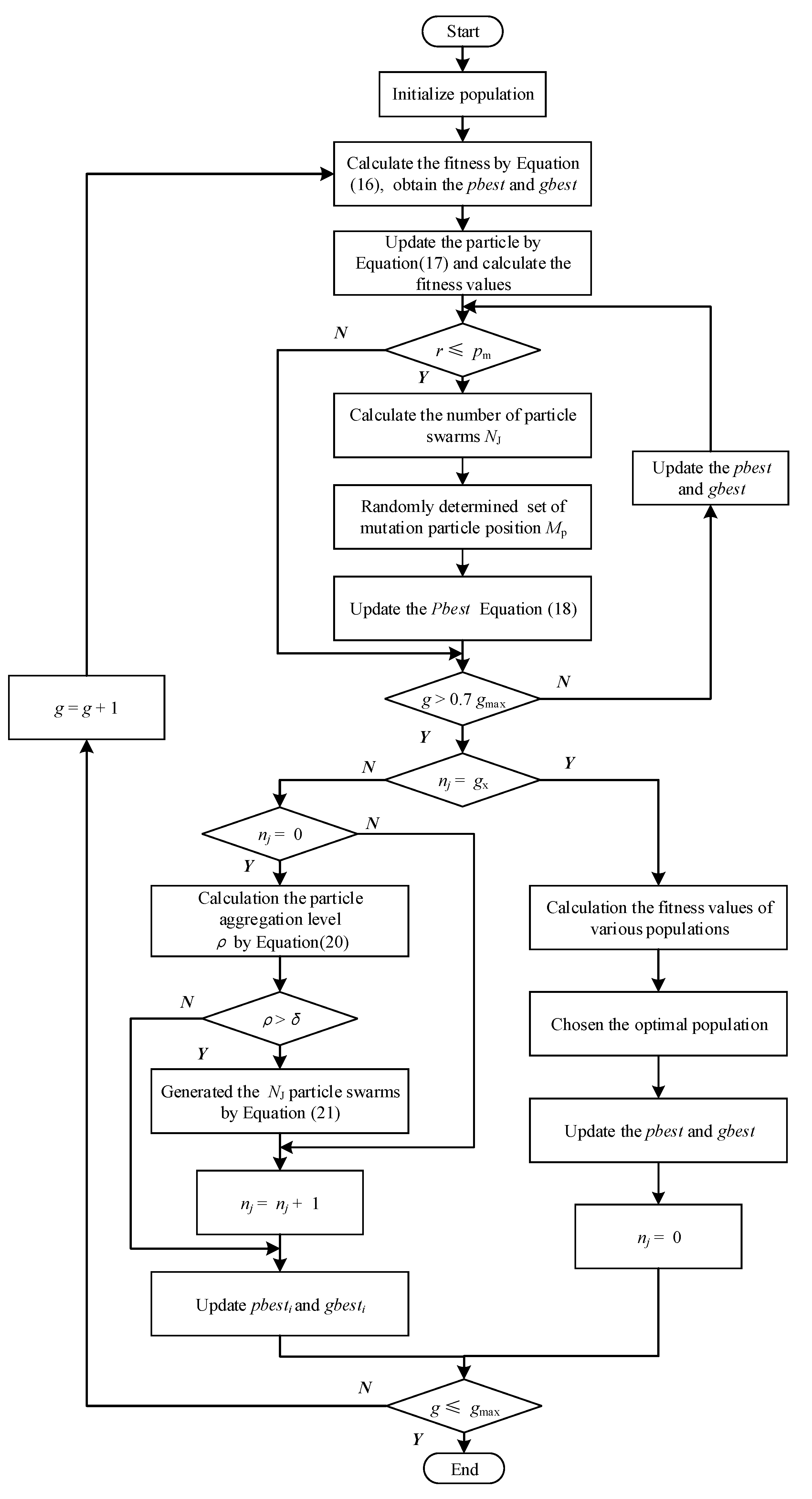
In the proposed EVMD, the minimum mean envelope entropy (MMEE) and enhanced particle swarm optimization (EPSO) algorithm are introduced in order to solve the optimal value of K and α and improve the computational convergence.

(2)

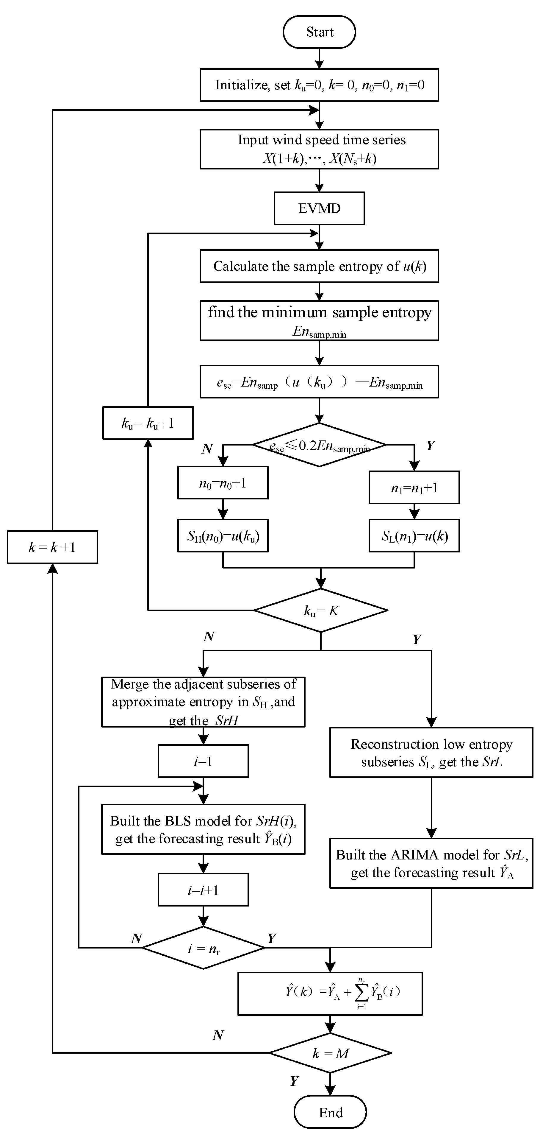
SR is applied to recombine the subseries obtained by EVMD. The sample entropy (SE) is used to quantify the complexity of the subseries, which are then adaptively divided into new high-entropy and low-entropy subseries. The adjacent high-entropy subseries of approximate entropy values are merged to obtain a new group of reconstructed high-entropy subseries, while the low-entropy subseries are merged into a new subseries as well.

(3)

A novel and robust hybrid prediction model (EVMD-SR-BLS-ARIMA) is proposed and employed for ultra-short-term wind power forecasting. This avoids the time-consuming training of a deep structures model. This paper introduces BLS, which is time-efficient and constantly updates the parameters of the forecasting model, to ultra-short-term wind speed forecasting. The forecasting results of nascent high- and low-entropy subseries are calculated using the BLS and ARIMA models. In order to improve the forecasting accuracy, an error-corrected EVMD-SR-BLS-ARIMA model is developed to post-process the errors.

The rest of the paper is organized as follows: Section 2 briefly reviews the related approaches involved in this paper; Section 3 describes the EVMD-SR-BLS-ARIMA model for wind speed forecasting in detail; Section 4 presents experimental simulations and comparative examples to demonstrate the performance of the proposed algorithm; finally, we present our conclusions in Section 5.

2. Related Work

In this section, the proposed methods are introduced, including the VMD and BLS network.

2.1. Variational Mode Decomposition

Variational mode decomposition (VMD) is an adaptive signal processing method first proposed by Konstantin Dragomiretskiy and Dominique Zosso [11]. VMD can decompose the original input signal, x(t), into a K intrinsic modes function (IMF), u_k(t) (k = 1, 2, …, K). In this process, the bandwidth sum of each mode is minimized, and the aggregation of modes u(t) is equal to the input signal, x(t). Compared with EMD, the instantaneous frequency of u(t) is physically meaningful, and is written as in Equation (1):

$$u_k(t)=A_k(t)\cos ({\Phi }_k(t))$$

(1)

where A_k(t) is the non-negative envelope of u_k(t), Φ_k is the phase, and the instantaneous frequency is the derivative of Φ_k.

VMD, completely different from EMD, transforms the signal decomposition process into a variational problem. Its adaptive decomposition is based on the optimal solution of the constrained variational problem, as described in Equation (2):

$$\underset{\left\{u_k\right\},\left\{{\omega }_k\right\}}{\min }\left\{{\displaystyle \sum _{k=1}^K{\Vert {\partial }_t\left[\left(\delta (t)+\frac{j}{\mathsf{\pi }t}\right)\ast u_k(t)\right]{\mathrm{e}}^{-j{\omega }_{k}t}\Vert }_2^2}\right\}\mathrm{s}.\mathrm{t}.{\displaystyle \sum _{k=1}^K{u}_k=x}$$

(2)

where u_k is the k-th IMF mode function, ω_k is the k-th center frequency, ∂_t is the partial derivative of the function for time t, δ(t) is the Dirac distribution, and ∗ indicates the convolution.

In order to find the optimal solution, the Lagrange multiplier λ and the quadratic penalty term α are introduced to Equation (2). Then, the constrained variational problem is turned into an unconstrained one, which can be expressed as in Equation (3):

$$\begin{array}{ll}\hfill L\left(\left\{u_k\right\},\left\{{\omega }_k\right\},\lambda \right)& =\alpha {\displaystyle \sum _{k=1}^K{\Vert {\partial }_t\left[\left(\delta (t)+\frac{j}{\mathsf{\pi }t}\right)\ast u_k(t)\right]{\mathrm{e}}^{-j{\omega }_{k}t}\Vert }_2^2}\hfill \\ & +{\Vert x(t)-{\displaystyle \sum _{k=1}^K{u}_k(t)}\Vert }_2^2+\langle \lambda (t),x(t)-{\displaystyle \sum _{k=1}^K{u}_k(t)}\rangle \hfill \\ \end{array}$$

(3)

Meanwhile, the alternating direction multiplier algorithm is employed to update the parameters of Equation (3) iteratively in order to calculate the saddle point of the Lagrange function. This process can be represented as in Equations (4) and (5) [16]:

$${\widehat{u}}_k^{n+1}(\omega )=\frac{\widehat{x}(\omega )-{\displaystyle \sum _{i\ne k}{\widehat{u}}_i(\omega )}+\frac{\widehat{\lambda }(\omega )}{2}}{1+2\alpha (\omega -{\omega }_k{)}^2}$$

(4)

$${\widehat{\omega }}_k^{n+1}=\frac{{\displaystyle {\int }_0^{\infty }\omega |{\widehat{u}}_k(\omega ){|}^2\mathrm{d}\omega }}{{\displaystyle {\int }_0^{\infty }|{\widehat{u}}_k(\omega ){|}^2\mathrm{d}\omega }}$$

(5)

where ${\widehat{u}}_k^{n+1}(\omega )$, ${\widehat{u}}_i(\omega )$, $\widehat{x}(\omega )$ and $\widehat{\lambda }(\omega )$ are the Fourier transforms of $u_k^{n+1}(t)$, $u_i(t)$, $x(t)$ and $\lambda (t)$, respectively, and n is the iteration number.

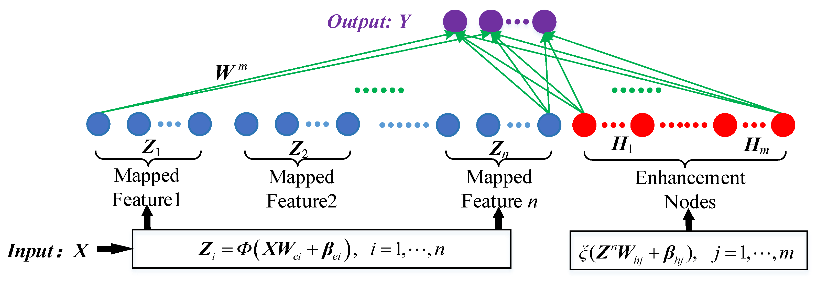
2.2. Broad Learning System

The broad learning system (BLS) is a kind of flat function-link neural network proposed by C. L. Philip Chen and Zhuliu Liu [17] which can overcome the time-consuming training process of deep-learning networks. The core concept of BLS is to transform the original input to the mapped feature (the mapped feature being an input of a function-link neural network) and to establish the enhancement node. In the BLS network, all mapping features and enhancement nodes are directly connected to the output; its structure is shown in Figure 1. The BLS network consists of mapped features, enhancement nodes, and an output layer.

Assuming that the BLS network sets n mapped features and each mapped feature is equipped with k nodes, the i-th mapped feature Z_i can be represented as in Equation (6):

$${\mathit{Z}}_i=\Phi (\mathit{X}{\mathit{W}}_{ei}+{\mathit{\beta }}_{ei}),i=1,\cdots ,n$$

(6)

where X is the input data, W_ei and β_ei are the random weights matrix and the random bias matrix of mapping feature, respectively, Φ(∙) is the nonlinear activation function, and Z_i is the output matrix.

Denoting all of the feature nodes of BLS as Z_n ≡ [Z₁, …, Z_n], the j-th enhancement node H_j can be defined as in Equation (7):

$${\mathit{H}}_j=\xi ({\mathit{Z}}^n{\mathit{W}}_{hj}+{\mathit{\beta }}_{hj}),j=1,\cdots ,m$$

(7)

where W_hj and β_hj are the random weights matrix and the random bias matrix of enhancement node, respectively, and ξ(∙) is the nonlinear activation function. Hence, in mathematical terms, the network output Y of the BLS can be denoted as in Equation (8):

$$\begin{array}{ll}\hfill \mathit{Y}& =\left[{\mathit{Z}}_1,\cdots ,{\mathit{Z}}_n|\xi ({\mathit{Z}}^n{\mathit{W}}_{h1}+{\mathit{\beta }}_{h1}),\cdots ,\xi ({\mathit{Z}}^n{\mathit{W}}_{hm}+{\mathit{\beta }}_{hm})\right]{\mathit{W}}^m\hfill \\ & =\left[{\mathit{Z}}_1,\cdots ,{\mathit{Z}}_n|{\mathit{H}}_1,\cdots ,{\mathit{H}}_m\right]{\mathit{W}}^m=\left[{\mathit{Z}}^n|{\mathit{H}}^m\right]{\mathit{W}}^m\hfill \end{array}$$

(8)

where W_m is the network connection weight matrix and W_m = [Z_n|H_m]⁺Y. [Z_n|H_m]⁺ is the Moore–Penrose inverse matrix of the matrix [Z_n|H_m], the value of which is estimated by ridge regression. Meanwhile, [Z_n|H_m]⁺ can be calculated using Equation (9):

$${\left[{\mathit{Z}}^n|{\mathit{H}}^m\right]}^{+}=\underset{\lambda \to 0}{\lim }(\lambda \mathit{I}+\left[{\mathit{Z}}^n|{\mathit{H}}^m\right]{\left[{\mathit{Z}}^n|{\mathit{H}}^m\right]}^{+}){\left[{\mathit{Z}}^n|{\mathit{H}}^m\right]}^T$$

(9)

As in a random vector function-link neural network, the network weights of BLS can be updated dynamically and quickly. Assuming that the initial network has n mapping features and m enhancement nodes and that the network input features matrix is ${\mathit{A}}_n^m$ = [Zⁿ|H^m], when denoting X_a as the new added data of BLS network the mapping features and enhancement nodes of the new added data are represented as in Equation (10):

$${\mathit{A}}_x=[\Phi ({\mathit{X}}_a{\mathit{W}}_{e1}+{\mathit{\beta }}_{e1}),\cdots ,\Phi ({\mathit{X}}_a{\mathit{W}}_{en}+{\mathit{\beta }}_{en}\left)\right|\xi ({\mathit{Z}}_x^n{\mathit{W}}_{h1}+{\mathit{\beta }}_{h1}),\cdots ,\xi ({\mathit{Z}}_x^n{\mathit{W}}_{hm}+{\mathit{\beta }}_{hm})]$$

(10)

where ${\mathit{Z}}_x^n$ = [Φ(X_aW_e1 + β_e1), …, Φ(X_aW_en + β_en)] is the mapping features matrix corresponding to X_a and W_ei, β_ei and W_hj, β_hj are randomly generated during the initialization of the network. Hence, the updated matrix of the output features, ${}^x\mathit{A}_n^m$, is provided by Equation (11):

$${}^x\mathit{A}_n^m=\left[\begin{array}{l}{\mathit{A}}_n^m\\ {\mathit{A}}_x^T\end{array}\right]$$

(11)

According to the Moore–Penrose inverse matrix recursive algorithm, the Moore–Penrose inverse matrix of the output features update matrix ${}^x\mathit{A}_n^m$ can be obtained as in Equation (12):

$${({}^x\mathit{A}_n^m)}^{+}=[{({\mathit{A}}_n^m)}^{+}+{\mathit{B}}^{\mathrm{T}}{\mathit{D}}^{\mathrm{T}}|{\mathit{B}}^{\mathrm{T}}]$$

(12)

where ${\mathit{D}}^T={\mathit{A}}_x^T{({\mathit{A}}_n^m)}^{+}$, ${\mathit{B}}^{\mathrm{T}}=\{\begin{array}{c}{({\mathit{A}}_x^T-{\mathit{D}}^T{\mathit{A}}_n^m)}^{+},{\mathit{A}}_x^T-{\mathit{D}}^T{\mathit{A}}_m\ne 0\\ (1+{\mathit{D}}^T\mathit{D}{)}^{-1}({\mathit{A}}_n^m{)}^{+}\mathit{D},{\mathit{A}}_x^T-{\mathit{D}}^T{\mathit{A}}_n^m=0\end{array}$.

Therefore, the new network weight matrix ${}^x\mathit{W}_x^m$ can be represented as in Equation (13):

$${}^x\mathit{W}_n^m={({}^x\mathit{A}_n^m)}^{+}{\mathit{Y}}_x$$

(13)

where Y_x is the network output and can be expressed as in Equation (14):

$${\mathit{Y}}_x=\left[\begin{array}{l}\mathit{Y}\\ {\mathit{Y}}_a\end{array}\right]$$

(14)

where Y_a is the output data corresponding to the new added data, X_a.

Based on Equations (8), (11), (12), and (14), the network weight matrix ${}^x\mathit{W}_x^m$ can be transformed as in Equation (15):

$${}^x\mathit{W}_n^m={\mathit{W}}_{}^m+({\mathit{Y}}_a^T-{\mathit{A}}_x^T{\mathit{W}}^m)\mathit{B}$$

(15)

3. EVMD-SR-BLS-ARIMA Hybrid Wind Speed Forecasting Model

In this section, a novel EVMD-SR-BLS-ARIMA hybrid wind speed forecasting model is developed that is able to attain high precision and efficiency.

3.1. Improved Variational Mode Decomposition (EVMD)

The non-linearity, non-smoothness and randomness of wind speed are the main factors that decrease accuracy in wind speed forecasting. VMD has the advantages of high computational efficiency and strong robustness, and can improve the smoothness of the original signal and reduce the complexity of modelling. Compared with the EMD, the values of IMF K and the quadratic penalty term α must be pre-set before using VMD. If the K value is too small, the feature of the original signal cannot be extracted efficiently. Conversely, excessive decomposition leads to added complexity in the model [18]. Furthermore, a smaller value of α results in the bandwidth of each obtained mode function being larger. Therefore, the choice of K and α directly affects the decomposition effect and reconstruction accuracy.

In order to address this problem, improved variational mode decomposition (EPSO-VMD, EVMD) is proposed, in which the minimum mean envelope entropy (MMEE) and enhanced particle swarm optimization (EPSO) algorithms are introduced in order to solve the optimal value of K and α and improve the computational convergence.

According to the characteristics of entropy, it is possible to use it to evaluate the sparsity of a signal. The amount of entropy can reflect the uniformity of a probability distribution [19]. Based on the entropy, the minimum mean envelope entropy (MMEE) of IMF is the objective function of the VMD parameter optimization algorithm. This objective function can be expressed as in Equation (16):

$$\underset{K,\alpha }{\min }F(K,\alpha )=-\frac{1}{K}{\displaystyle \sum _{k=1}^K{\displaystyle \sum _{i=1}^N{p}_i{\log }_2(p_i)}},\hspace{1em}\hspace{1em}\hspace{1em}\hspace{1em}{p}_i=h(i)/{\displaystyle \sum _{i=1}^{N}h(i)}$$

(16)

where h is the envelope of the mode function u_k generated by the Hilbert transform and p_i is the probability at the i-th point of the envelope.

In order to improve convergence, an enhanced particle swarm optimization (EPSO) algorithm is proposed to solve the optimal parameters of VMD in this paper. In ordinary PSO, the velocity and position of each particle in PSO-updating rules are provided as in Equation (17) [20]:

$$\{\begin{array}{l}{v}_i(g+1=w{v}_i(g)+c_1{r}_1(pbes{t}_i-x_i(g)+c_2{r}_2(gbest-x_i(g))\\ x_i(g+1=x_i(g)+v_i(g+1)\end{array}$$

(17)

where pbest_i is the best solution of particle i, gbest is the optimal solution of the entire swarm, g is an iteration number, v_i (g) is velocity, x_i (g) is the position of particle i at iteration g, w is an inertia weight, c₁ and c₂ are learning factors, and r₁ and r₂ are random numbers in [0, 1].

In order to improve the global search ability, the EPSO adds mutation and jump operations in the search process. At each iteration, this algorithm can randomly determine the mutation number and position of an individual optimal solution pbest with a certain mutation probability, and this probability gradually decreases as the iterations proceed. Thus, the pbest updating rule for population number N_p is defined as in Equation (18):

$$\begin{array}{l}pbest=\{\begin{array}{l}pbest,\hspace{1em}\hspace{1em}r>p_{\mathrm{m}}\\ R_{pbest},\hspace{1em}\hspace{1em}r\le p_{\mathrm{m}}\end{array}\\ R_{pbest}(i)=\{\begin{array}{l}pbest(i),\hspace{1em}\hspace{1em}i\notin M_{\mathrm{p}}\\ rand,\hspace{1em}\hspace{1em}i\in M_{\mathrm{p}}\end{array},\hspace{1em}\hspace{1em}i=1,2,\cdots N_{\mathrm{p}}\end{array}$$

(18)

where p_m is the mutation probability, M_p is the randomly determined set of mutation particle positions in pbest, and r is a random number in [0, 1].

At each iteration, the number of elements nm in the set M_p is generated randomly, and n_m ≤ N_p/2. Then, the mutation probability p_m is satisfied as in Equation (19):

$$p_{\mathrm{m}}=p_{\mathrm{m},\max }-\frac{(g-1)(p_{\mathrm{m},\max }-p_{\mathrm{m},\min })}{(g_{\max }-1)}$$

(19)

where p_m,min is the minimum mutation probability, p_m,max is the maximum mutation probability, and g_max is the maximum iteration number.

In later iterations a large number of particles concentrates in a narrow area and the optimization result easily falls into local optimization, from which it is difficult to emerge. Compared with PSO, the multiple uniformly distributed particle populations are regenerated near the current optimal solution via the jump operation and the new optimal solution is obtained via multi-step iterative competition. In this paper, the later iteration is defined as g > 0.7 g_max. Meanwhile, the particle aggregation level is used as the trigger threshold in the jump operation, which can be expressed as in Equation (20):

$$\begin{array}{l}\rho =\frac{1}{N_{\mathrm{p}}d}{\displaystyle \sum _{i=1}^{N_{\mathrm{p}}}{\displaystyle \sum _{j=1}^d\eta (x_{i,j}(g))}}\\ \eta (x_{i,j}(g))=\{\begin{array}{l}1,\hspace{1em}\hspace{1em}(|x_{i,j}(g)-gbest|/|gbest|)<\epsilon \\ 0,\hspace{1em}\hspace{1em}\mathrm{others}\end{array}\end{array}$$

(20)

where ρ is the particle aggregation level and ε is a small positive number.

If ρ > δ, N_J particle swarms are generated, the h-th particle swarm is as provided in Equation (21):

$$x_{i,j}^h(g+1)=\{\begin{array}{l}gbest+r(x_{\max }(g)-gbest),\hspace{1em}\hspace{1em}(x_{\max }(g)-gbest)>(gbest-x_{\min }(g))\\ gbest+r(gbest-x_{\min }(g)),\hspace{1em}\hspace{1em}\mathrm{others}\end{array}$$

(21)

where h is the number of the new generated particle swarms (h = 1,2, …, N_J), r is the random number in [0, 1], x_max(g) is the maximum value of x_i,j at the g-th iteration, and x_min(g) is the minimum value of x_i,j at the g-th iteration.

After g_x iterations and optimizations of N_J particle swarms by Equation (21), the population with the best solution continues to the next iteration to update the global best solution. The introduced random value within a range can increase the population diversity and avoid early maturity. A flowchart representing the EPSO optimization algorithm is shown in Figure 2.

3.2. Subseries Reconstruction Method (SR)

The structure of the traditional decomposition–combination wind speed forecasting model is shown in Figure 3. Here, each subseries must be modelled independently, which increases the model’s complexity and calculation time. In order to improve the accuracy and efficiency of the forecasting model, this paper proposes a subseries reconstruction (SR) method to satisfy the accuracy and timeliness requirements for ultra-short-term wind speed forecasting. In SR, the sample entropy (SE) is introduced to quantify the EVMD subseries complexity, while the reconstruction method of adjacent subseries with approximate entropy is proposed to decrease the number of subseries.

Formally, the sample entropy of time series {x_i} (i = 1, …, N) can be expressed as in Equation (22):

$$E{n}_{\mathrm{samp}}=-\ln \left[\frac{B^{m+1}(r)}{B^m(r)}\right]$$

(22)

where m is the dimension of vector sequences, r is the similarity tolerance, and B^m(r) is the mean of the number of distances between all vectors less than or equal to r, which can be expressed as in Equation (23):

$$\begin{array}{c}{B}^m(r)=\frac{1}{N-m+1}{\displaystyle \sum _{i=1}^{N-m+1}{B}_i^m(r})\\ B_i^m(r)=\frac{1}{N-m}C\left\{\mathrm{d}\right[X(i),X(j)]<r\},i=1,2,\cdots N-m+1,i\ne j\end{array}$$

(23)

where X(i) is m dimensional sequences composed of {x_i} in order, X(i) = [x(i), …, x(i + m − 1)] (i = 1, 2, …, N − m + 1), d[X(i), X(j)] are the absolute maximum distance between vector X(i) and X(j), and C{∙} is a function that counts the number of vectors that satisfy the condition.

Based on Equation (23), m and r are critical in determining the outcome of sample entropy. In most conditions, the value of m is 1 or 2, and r is in [0.1SD, 0.25SD], where SD is the standard deviation of the original time series {x_i} [21]. The sample entropy value of {x_i} is related to the series complexity; the higher the series complexity, the higher the sample entropy value.

In the series reconstruction method, the complexity of EVMD subseries of the original wind speed time series is assessed by sample entropy and the subseries are sorted from lowest to highest according to entropy value. Setting the threshold of entropy, the EVMD subseries are adaptively divided into high-entropy subseries, S_H, and low-entropy subseries, S_L. Evaluating the entropy of adjacent high-entropy subseries, the adjacent subseries with approximate entropy values are merged, then a new group of reconstructed high-entropy subseries, SrH, is obtained. Meanwhile, the low-entropy subseries merge into another new subseries, SrL. Because the complexity of the merged subseries approximates the original subseries, this reconstructed subseries method can improve accuracy and efficiency. The framework of this method is shown in Figure 4.

3.3. Hybrid Wind Speed Forecasting Framework

The EVMD-SR-BLS-ARIMA hybrid wind speed forecasting model proposed in this paper mainly includes data on time–frequency analysis, subseries reconstruction, hybrid model construction, and linear superposition of prediction results in four major parts; the framework is shown in Figure 5. First, the EVMD is utilized to decompose the original wind speed time series in order to obtain K subseries, thereby reducing irregularities. Second, SR is applied to reconstruct the subseries in order to decrease their number and improve forecasting efficiency. Subsequently, the BLS-ARIMA model is used to forecast different reconstructed subseries. Finally, the final forecasting result is obtained by linear superposition of the forecasting values of each subseries.

As shown in Figure 6, the forecasting process of the EVMD-SR-BLS-ARIMA forecasting model is as follows:

Step 1: Initialize the number of forecasting cycles k, k_u, n₀, n₁, and n_r to 0; set the input model wind speed time series length, N_s, and forecasting times, M.

Step 2: Using the EVMD method, the wind speed time series [X(1 + k), …, X(N_s + k)] is decomposed into K subseries u(k); calculate the sample entropy of each subseries and find the minimum sample entropy, En_samp,min.

Step 3: Using 1.2En_samp,min as the threshold, divide the subseries u(k) into the high-entropy subseries S_H and low-entropy subseries S_L, then count the numbers of high-entropy subseries n₀ and low-entropy subseries n₁.

Step 4: The adjacent subseries with no more than 10% En_samp variation in S_H are reconstructed to obtain a new group of high-entropy subseries SrH (the number of SrH is n_r) and the forecasting results Ŷ_B(i) (I = 1, …, n_r) are calculated via the BLS model. The n₁ low-entropy subseries, S_L, merge into a new subseries, SrL, and an ARIMA model for SrL is built to obtain the forecasting result Ŷ_A; then, the k-th wind speed forecasting result is $\widehat{Y}(k)={\widehat{Y}}_{\mathrm{A}}+{\displaystyle \sum _{i=1}^{n_r}{\widehat{Y}}_{\mathrm{B}}(i)}$.

Step 5: k = k + 1. Repeat steps 2–4 until k = M is reached at the end of the forecasting process and the M-step forecasting results are obtained.

In order to improve forecasting accuracy, the error-corrected EVMD-SR-BLS-ARIMA model is developed to post-process the errors. This error-corrected model is essentially a two-stage forecasting model. The first stage is composed of EVMD-SR-BLS-ARIMA for wind speed basis data, which calculates the forecasting error calculated, while the second stage uses ARIMA to calculate the forecasting error of the EVMD- SR-BLS-ARIMA model. In the forecasting process, the second-level model is used to correct the first-level prediction data in order to obtain the final prediction result.

3.4. Evaluation Index

In order to quantitatively evaluate the performance of the forecasting model, the Root Mean Square Error (RMSE), Mean Absolute Error (MAE), and symmetric Mean Absolute Percentage Error (sMAPE) are introduced. The discrepancy between anticipated and actual values is measured by these three indicators, with lesser values indicating better forecast accuracy. Respectively, the three evaluation indexes are defined as in Equations (24)–(26):

$${\delta }_{\mathrm{RMSE}}=\sqrt{\frac{1}{N}{\displaystyle \sum _{t=1}^N(y_t-{\widehat{y}}_t{)}^2}}$$

(24)

$${\delta }_{\mathrm{MAE}}=\frac{1}{N}{\displaystyle \sum _{t=1}^N\left|y_t-{\widehat{y}}_t\right|}$$

(25)

$${\delta }_{\mathrm{sMAPE}}=\frac{1}{N}{\displaystyle \sum _{t=1}^N\frac{2\left|y_t-{\widehat{y}}_t\right|}{y_t+{\widehat{y}}_t}\times 100\%}$$

(26)

where y_t is the actual value at time t, ŷ_t is the predicted value at time t, and N is the observation size.

4. Case Study

In this section, original wind speed data from a Huaneng Group wind farm in Shandong province from 1 January 2016 were used to test the accuracy of the ultra-short-term wind speed forecasting method. The wind forecasting model was constructed using m-files in MATLAB R2016b running on a Windows PC with an Intel I5-8500 CPU.

4.1. Data Collection

The sample data were based on actual test data from a 1.5 MW wind turbine supervisory control and data acquisition (SCADA) system with a the sampling period of 10 min (24 h total, 144 sampling points [X₁, …, X₁₄₄]). The sample wind speed time series is shown in Figure 7. The average wind speed in the sample was 6.72 m/s, the maximum wind speed was 11.80 m/s, and the minimum wind speed was 2.08 m/s. The wind speed sequence fluctuated noticeably with no discernible pattern. In this case study, the first 100 sampling points (sampling points 1~100) of the wind speed series were utilized as modeling data, while the next 44 points (sampling points 101~144) were used as test samples to evaluate the prediction model’s accuracy and timeliness.

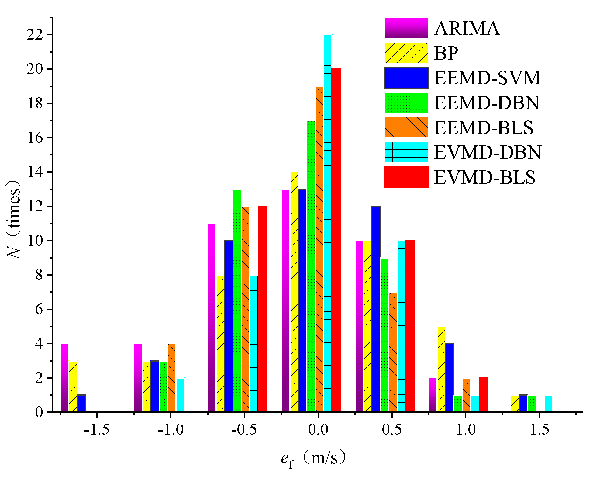
4.2. Experiment 1: EVMD-BLS Forecasting Model

Experiment 1 mainly studied the ultra-short-term wind speed forecasting performance of the EVMD-BLS decomposition–combination model. In this model, the EVMD divides the wind speed time series into subseries with simple frequency components and more regular variation, creates the BLS models of each subseries, and then constructs the error correction model for increased accuracy. Meanwhile, when the wind speed time series N_s in the input model is set to 70, the first 100 wind speed samples are divided into two parts: the first 70 data points are used for wind speed forecasting, and the last 30 are used for error modeling.

According to the method introduced in Section 3.1, the EPSO algorithm was used to solve the optimal values of K and α in the EVMD method. In order to prevent excessive variation from destroying the algorithm’s convergence efficiency, the size of the set of variation particles, M_p, was limited to within 50% of the population particle number N_p. Taking into account the algorithm’s computational efficiency, the start point of the jump operation was set to 70% of the maximum number of iterations. Additionally, the particle aggregation level calculation limit ε in Equation (20) was set to 0.01, the aggregation trigger limit, δ, was 0.5, IMF K was an integer between 1 and 10, and the quadratic penalty term α was a value between 1 and 50. The EPSO optimization algorithm parameters were set as shown in

Table 1. Parameters of the EPSO optimization algorithm.

Parameter	Np	wmin	wmax	c1	c2	pm,min	pm,max
Value	30	0.4	0.9	1.497	1.497	0.1	0.6

.

Figure 8 depicts the variation curve of the minimum average envelope entropy value in the EPSO optimal value search with the number of iterations, g; the parameters of variational mode decomposition are then determined as K = 6 and α = 5.67.

The first 70 wind speed data points were subjected to EVMD to generate six mode functions (u₁, …, u₆), as shown in Figure 9. In order to compare the validity of decomposition, the wind speed data were decomposed using ensemble empirical mode decomposition (EEMD). When the standard deviation of Gaussian white noise was set to 0.4 and the noise order was set to 50 in EEMD, the wind speed data were decomposed into five IMF components and one residual component, r, as shown in Figure 10.

Analyzing the characteristics of each component of EVMD and EEMD, the highest frequency component’s amplitude in EVMD is between [−0.35, 0.40], with a component mean of −0.01, and the highest frequency component’s amplitude in EEMD is between [−0.93, 0.83], with a component mean of 0.03. Compared with EEMD, it is evident that EVMD decomposes the high-frequency component more completely. When the waveforms of the lowest frequency component generated by the two approaches are compared, the lowest frequency component of EVMD can better depict the long-term fluctuation features of the wind speed.

The BLS forecasting model was used for each EVMD subseries of the first 70 wind speed data points, and the forecasting result at the 71st point was derived. We updated the input data and performed the EVMD-BLS forecasting procedure 30 times to obtain the expected wind speeds at the 71st to 100th points, calculate the forecast error at the 71st to 100th points, and obtain the forecasting error series. The ARIMA model for the error series was constructed in order to calculate the error forecasting value at the 101st point. Meanwhile, the corrected forecasting result of the 101st point was obtained by superimposing the 101st point of EVMD-BLS and the error forecasting results for the same point.

To validate the prediction performance of the EVMD-BLS model, the ARIMA, BP, EEMD-SVM, EEMD-DBN, EEMD-BLS, and EVMD-DBN models were employed for comparison.

In this paper, the mapping features of the BLS model are set to 30, each mapping feature contains 100 nodes, and the enhanced nodes are set to 300. The DBN network structure is set to 100-500-500-100. The simulation experiment employed these seven models to predict ultra-short-term wind speed at the 101st to 144th points, with the results are presented in Figure 11.

The wind speed forecast results of the seven models are generally similar to the actual wind speed fluctuation trends, and EEMD-DBN, EEMD-BLS, EVMD-DBN, and EVMD-BLS are better at tracking actual wind speed variation. We used the RMSE, MAE, and sMAPE to evaluate the forecasting performance of these models; the results are shown in

Table 2. Evaluation result of seven forecasting models.

Model	δRMSE (m/s)	δMAE (m/s)	δsMAPE (%)	t (s)
ARIMA	0.64	0.54	12.19	91.07
BP	0.68	0.53	12.77	101.85
EEMD-SVM	0.62	0.48	12.24	226.43
EEMD-DBN	0.46	0.37	9.49	478.99
EEMD-BLS	0.49	0.37	9.20	203.01
EVMD-DBN	0.46	0.34	8.85	235.92
EVMD-BLS	0.38	0.31	7.85	190.45

.

In comparing the evaluation index of the seven models, the forecasting models using time–frequency analysis perform significantly better than the ARIMA and BP models. Among the three EEMD forecasting models, the EEMD-DBN and EEMD-BLS models outperform the EEMD-SVM model, while the EEMD-BLS model has the faster running speed. In both of the models using DBN, the EVMD-DBN model has higher prediction accuracy and efficiency than the EEMD-DBN model; however, the amplitude of the high-frequency component of the EEMD is large, and affects overall prediction accuracy. Furthermore, the Gaussian white noise introduced by the EEMD in signal decomposition increases computation time. Compared to the EVMD-DBN model, the EVMD-BLS model has higher wind speed forecasting accuracy and can greatly reduce computing time. Statistical analysis of the forecasting errors of the seven models was performed, and the results are presented in Figure 12.

For the seven combined models, the distribution of ultra-short-term wind speed prediction errors is as follows: (1) The percentage of prediction errors in the (−0.5, 0.5) interval is 29.54% for the ARIMA model, 29.54% for the EEMD-SVM model, 38.63% for the EEMD-DBN model, 43.18% for the EEMD-BLS model, 50% for the EVMD-DBN model, and 45.45% for the EVMD-BLS model; (2) The percentage of prediction errors in the (−1.0, 1.0) interval is 81.81% for the ARIMA model, 86.36% for the EEMD-SVM model, 93.18% for the EEMD-DBN model, 90.91% for the EEMD-BLS model, 93.18% for the EVMD-DBN model, and 100% for the EVMD-BLS model. Therefore, the prediction errors of the EVMD-BLS model are all less than 1 m/s, and the computing time is short.

The Diebold–Mariano (DM) test is introduced to further evaluate the validity of the forecasting model in this paper. The DM test results of the seven forecasting models are shown in

Table 3. Evaluation result of forecasting models.

		BP	EEMD-SVM	EEMD-DBN	EEMD-BLS	EVMD-DBN	EVMD-BLS
p-value	ARIMA	0.647	0.597	0.018	0.03	0.015	0.003
	BP	/	0.476	0.015	0.036	0.007	0.003
	EEMD-SVM	/	/	0.107	0.17	0.102	0.021
	EEMD-DBN	/	/	/	0.445	0.986	0.014
	EEMD-BLS	/	/	/	/	0.559	0.034
	EVMD-DBN	/	/	/	/	/	0.088
DM-value	ARIMA	−0.461	0.533	2.467	2.239	2.524	3.195
	BP	/	0.719	2.547	2.167	2.807	3.195
	EEMD-SVM	/	/	1.646	1.397	1.67	2.389
	EEMD-DBN	/	/	/	−0.771	−0.017	2.565
	EEMD-BLS	/	/	/	/	0.589	2.191
	EVMD-DBN	/	/	/	/	/	1.744

.

According to the DM test method, the tested model’s accuracy is better than the reference model when the p-value is <0.05 and the DM value is >0. As shown in Table 3, except for the BP model, the forecasting accuracy of ARIMA is lower than the other five models. In particular, the EVMD-BLS method proposed in this paper significantly outperforms the ARIMA, BP, EEMD-SVM, EEMD-DBN, and EEMD-BLS models. Compared with the EVMD-DBN model, the p-value of 0.088 from the DM test of the EVMD-BLS model is very close to the threshold of significant difference (0.05), and its time, error statistics, and three evaluated indexes are better than those of EVMD-DBN.

4.3. Experiment 2: EVMD-SR-BLS-ARIMA Hybrid Forecasting Model

According to the method introduced in Section 3.2 and Section 3.3, the EVMD-SR-BLS-ARIMA hybrid model was used to forecast the ultra-short-term wind speed of wind farms, with the 101st point in the forecasting process used as an example to demonstrate the modeling.

With the input wind speed data length N_s set to 100, the input wind speed data are [X₁, …, X₁₀₀].

The EPSO algorithm was used to solve the optimization parameters K and α as 7 and 6.40, respectively, and the input data were decomposed by the EVMD to obtain seven subseries (u₁, …, u₇), as shown in Figure 13a. Using sample entropy (SE) to evaluate the complexity of the decomposed subseries, the SE evaluation parameters m and r were set to 2 and 0.2 SD (standard deviation), respectively; the SE results for each subseries are presented in Figure 14.

In Figure 14, the horizontal axis u value of 0 represents the sample entropy of the undecomposed wind speed data, u₀. The sample entropy values of each subseries u₁~u₇ are 60.32%, 73.68%, 63.47%, 61.56%, 71.10%, 20.22% and 21.69% of the sample entropy value of u₀, respectively, and the minimum sample entropy, En_samp,min, is 0.299. The high-entropy-value subseries were screened as u₁~u₅ and the low-entropy-value sequences as u6 and u₇ using the method shown in Figure 6, with 1.2 En_samp,min as the threshold. The subseries u₆ and u₇ were reconstructed as the new subseries SrL, and the adjacent high-entropy subseries were reconstructed with the requirement that the change in En_samp did not exceed 10%. The reconstructed subseries are shown in Figure 13b. The nascent subsequence SrH₁ is u₁, SrH₂ is u₂, SrH₃ is u₃ combined with u₄, SrH₄ is u₅, and SrL is u₆ fused with u₇. In the EVMD-SR-BLS-ARIMA model, the forecasting results of the nascent high-entropy subseries SrH are calculated by the BLS model, while the ARIMA model obtains the forecasting result of the new low-entropy subseries.

The simulation experiment employed the EVMD-SR-BLS-ARIMA model to predict ultra-short-term wind speed at the 101st to 144th points, with the results presented in Figure 15. The green dotted lines with triangle symbols represent the EVMD-SR-BLS-ARIMA model’s forecasting results, while the red dashed lines with dots represent the results of the error-corrected EVMD-SR-BLS-ARIMA model. Wind speed variations can be tracked with excellent precision using these two models; their forecasting evaluation results are shown in

Table 4. Evaluation indexes by EVMD-SR-BLS-ARIMA model.

Model	δRMSE (m/s)	δMAE (m/s)	δsMAPE (%)	t (s)
EVMD-SR-BLS-ARIMA	0.45	0.32	8.25	126.94
Error-corrected EVMD-SR-BLS-ARIMA	0.34	0.30	7.99	172.67

.

The forecasting accuracy of the EVMD-SR-BLS-ARIMA model is similar to that of the EVMD-BLS model, and is better than the other models, as shown in Table 3. Due to the complexity of evaluating the wind speed decomposition subseries using sample entropy, the low-entropy series is passed to the ARIMA model for processing, and the adjacent approximate high-entropy series are reconstructed to reduce the model size and computational time.

The model calculation time is decreased from 190.45 s in the EVMD-BLS model to 126.94 s, which is just 66.65% of the EVMD-BLS model’s calculation time. The δ_RMSE, δ_MAP, and δ_MAPE of the error-corrected EVMD-SR-BLS-ARIMA model are 0.34 m/s, 0.30 m/s, and 8.38%, respectively, and its computation time is 90.66% of that of the EVMD-BLS model. To summarize, the EVMD-SR-BLS-ARIMA model can provide an excellent balance of accuracy and efficiency in wind speed forecasting.

The statistical analysis results of the forecasting error of the two reconstructed models are shown in Figure 16. It can be observed that (1) the EVMD-SR-BLS-ARIMA model’s forecasting error is [−1.33, 1.04], the probability that the forecasting error is in the (−1.0, 1.0) interval is 93.18%, and the probability that the forecasting error is in the (−0.5, 0.5) interval is 68.18%; (2) the error-corrected EVMD-SR-BLS-ARIMA model’s forecasting error is [−0.68, 0.55], and the probability that the forecasting error is in the (−0.5, 0.5) interval is 84.09%.

This paper used two different days of wind speed data from the same wind farm (collected on 6 and 13 January 2016) to verify the applicability of the model; the results are shown in Figure 17. Compared with the ARIMA model, the p-value and DM-value of the error-corrected EVMD-SR-BLS-ARIMA model are 0.045 and 2.057, and its δ_sMAPE is 7.41% less than that of ARIMA (10.58%) for 6 January 2016; the p-value and DM-value of the error-corrected EVMD-SR-BLS-ARIMA model are 0.033 and 2.20, and its δ_sMAPE is 6.62% less than that of ARIMA (7.73%) for 13 January 2016. Hence, the proposed model has better applicability.

According to the above experimental simulation results, it can be observed that (1) the proposed model has higher prediction accuracy and stronger prediction performance; and (2) the proposed model can significantly improve computational operation efficiency and reduce the time required to completion.

5. Conclusions

In view of the fact that actual wind speed is affected by weather, temperature, and random factors, there are a large number of outliers in wind speed prediction and it is strongly nonlinear. In this study, a hybrid intelligent forecasting model for ultra-short-term wind speed forecasting based on EVMD, SR, and BLS is proposed. The conclusions of this paper can be listed as follows:

• EVMD was used to decompose the wind speed time series, while the minimum mean envelope entropy (MMEE) and enhanced particle swarm optimization (EPSO) algorithms were introduced to attain the optimal values of K and α of EVMD.
• SR was applied to recombine the subseries obtained by EVMD. The subseries of EVMD were adaptively divided into high-entropy and low-entropy subseries. Adjacent high-entropy subseries of approximate entropy values were merged to obtain a new group of reconstructed high-entropy subseries, and the low-entropy subseries were merged into a new subseries as well.
• The EVMD-SR-BLS-ARIMA hybrid wind speed forecasting model was constructed to obtain the reconstructed subseries forecasting results. Experimental results showed that the proposed method can significantly improve the forecasting accuracy and reduce the time required.

In future research, we intend to select more appropriate models for wind speed datasets with different features, investigate forecasting results with a nonlinear weighted combination of components, improve forecasting accuracy characteristics from the standpoint of BLS structure, optimize this model to carry out wind power forecasting, and identify the optimal configuration of the energy storage system capacity of wind power systems.

References

1. Liu, H.; Chen, C. Data Processing Strategies in Wind Energy Forecasting Models and Applications: A Comprehensive Review. Appl. Energy 2019, 249, 392–408. [Google Scholar] [CrossRef]
2. Zuo, H.; Bi, K.; Hao, H. A State-of-the-Art Review on the Vibration Mitigation of Wind Turbines. Renew. Sustain. Energy Rev. 2020, 121, 109710. [Google Scholar] [CrossRef]
3. Tascikaraoglu, A.; Uzunoglu, M. A Review of Combined Approaches for Prediction of Short-Term Wind Speed and Power. Renew. Sustain. Energy Rev. 2014, 34, 243–254. [Google Scholar] [CrossRef]
4. Okumus, I.; Dinler, A. Current Status of Wind Energy Forecasting and a Hybrid Method for Hourly Predictions. Energ. Convers. Manag. 2016, 123, 362–371. [Google Scholar] [CrossRef]
5. Tascikaraoglu, A.; Sanandaji, B.M.; Poolla, K.; Varaiya, P. Exploiting Sparsity of Interconnections in Spatio-Temporal Wind Speed Forecasting Using Wavelet Transform. Appl. Energy 2016, 165, 735–747. [Google Scholar] [CrossRef] [Green Version]
6. Wang, H.Z.; Wang, G.B.; Li, G.Q.; Peng, J.C.; Liu, Y.T. Deep Belief Network Based Deterministic and Probabilistic Wind Speed Forecasting Approach. Appl. Energy 2016, 182, 80–93. [Google Scholar] [CrossRef]
7. Liu, H.; Tian, H.; Li, Y. An Emd-Recursive Arima Method to Predict Wind Speed for Railway Strong Wind Warning System. J. Wind Eng. Ind. Aerod. 2015, 141, 27–38. [Google Scholar] [CrossRef]
8. An, N.; Zhao, W.; Wang, J.; Shang, D.; Zhao, E. Using Multi-Output Feedforward Neural Network with Empirical Mode Decomposition Based Signal Filtering for Electricity Demand Forecasting. Energy 2013, 49, 279–288. [Google Scholar] [CrossRef]
9. Huang, Y.; Yang, L.; Liu, S.; Wang, G. Multi-Step Wind Speed Forecasting Based on Ensemble Empirical Mode Decomposition, Long Short Term Memory Network and Error Correction Strategy. Energies 2019, 12, 1822. [Google Scholar] [CrossRef] [Green Version]
10. Sun, B.; Yao, H. Short-Term Wind Speed Forecasting Based on Local Mean Decomposition and Multi-Kernel Support Vector Machine. Acta Energ. Solaris Sin. 2013, 34, 1567–1573. [Google Scholar]
11. Dragomiretskiy, K.; Zosso, D. Variational Mode Decomposition. IEEE Trans. Signal. Process 2014, 62, 531–544. [Google Scholar] [CrossRef]
12. Sun, W.; Gao, Q. Short-Term Wind Speed Prediction Based on Variational Mode Decomposition and Linear–Nonlinear Combination Optimization Model. Energies 2019, 12, 2322. [Google Scholar] [CrossRef] [Green Version]
13. Han, L.; Zhang, R.; Wang, X.; Bao, A.; Jing, H. Multi-Step Wind Power Forecast Based on Vmd-Lstm. Iet Renew. Power Gen. 2019, 13, 1690–1700. [Google Scholar] [CrossRef]
14. Zhu, L.; Lian, C. Wind Speed Forecasting Based on a Hybrid Emd-Bls Method; Institute of Electrical and Electronics Engineers Inc.: Hangzhou, China, 2019; pp. 2191–2195. [Google Scholar]
15. Zhu, L.; Lian, C.; Zeng, Z.; Su, Y. A Broad Learning System with Ensemble and Classification Methods for Multi-Step-Ahead Wind Speed Prediction. Cogn. Comput. 2020, 12, 654–666. [Google Scholar] [CrossRef]
16. Bai, Y.; Liu, M.; Ding, L.; Ma, Y. Double-Layer Staged Training Echo-State Networks for Wind Speed Prediction Using Variational Mode Decomposition. Appl. Energy 2021, 301, 117461. [Google Scholar] [CrossRef]
17. Chen, C.L.P.; Liu, Z. Broad Learning System: An Effective and Efficient Incremental Learning System without the Need for Deep Architecture. IEEE Trans Neur. Net. Learn. 2018, 29, 10–24. [Google Scholar] [CrossRef] [PubMed]
18. Zhang, G.; Liu, H.; Zhang, J.; Yan, Y.; Zhang, L.; Wu, C.; Hua, X.; Wang, Y. Wind Power Prediction Based on Variational Mode Decomposition Multi-Frequency Combinations. J. Mod. Power Syst. Clean 2019, 7, 281–288. [Google Scholar] [CrossRef] [Green Version]
19. Tang, G.; Wang, X. Parameter Optimized Variational Mode Decomposition Method with Applicaltion to Incipient Fault Diagnosis of Rolling Bearing. J. Xi’an Jiaotang Univ. 2015, 49, 73–81. [Google Scholar]
20. Ramadan, H.S.; Bendary, A.F.; Nagy, S. Particle Swarm Optimization Algorithm for Capacitor Allocation Problem in Distribution Systems with Wind Turbine Generators. Int. J. Electr. Power Energy Syst. 2017, 84, 143–152. [Google Scholar] [CrossRef]
21. Alcaraz, R.; Rieta, J.J. A Review on Sample Entropy Applications for the Non-Invasive Analysis of Atrial Fibrillation Electrocardiograms. Biomed. Signal. Proces. 2010, 5, 1–14. [Google Scholar] [CrossRef]
Figure 1. Structure of the broad learning system.
Energies 15 04492 g001
Figure 2. Flowchart of EPSO optimization algorithm.
Energies 15 04492 g002
Figure 3. Framework of traditional decomposition–combination wind speed forecasting model.
Energies 15 04492 g003
Figure 4. Framework of subseries reconstruction method.
Energies 15 04492 g004
Figure 5. The framework of the EVMD-SR-BLS-ARIMA hybrid wind speed forecasting model.
Energies 15 04492 g005
Figure 6. Flowchart of EVMD-SR-BLS-ARIMA for ultra-short-term wind speed forecasting.
Energies 15 04492 g006
Figure 7. Sample of wind speed time series.
Energies 15 04492 g007
Figure 8. Iterative process of variational mode decomposition parameter optimization.
Energies 15 04492 g008
Figure 9. EVMD results of the first 70 points in the wind speed series.
Energies 15 04492 g009
Figure 10. Ensemble empirical mode decomposition results of the first 70 points of the wind speed series.
Energies 15 04492 g010
Figure 11. Wind speed forecasting results of seven different models.
Energies 15 04492 g011
Figure 12. Forecasting-error statistics of seven models.
Energies 15 04492 g012
Figure 13. Decomposition result of the first 100 points in the wind speed series: (a) result of EVMD and (b) result of subseries reconstruction.
Energies 15 04492 g013
Figure 14. Subseries sample entropy of EVMD.
Energies 15 04492 g014
Figure 15. Wind speed forecasting results of EVMD-SR-BLS-ARIMA model.
Energies 15 04492 g015
Figure 16. Forecasting errors and statistics of EVMD-SR-BLS-ARIMA models: (a) forecasting error and (b) error statistics.
Energies 15 04492 g016
Figure 17. Wind speed forecasting results at different times: (a) 6 January 2016 and (b) 13 January 2016.
Energies 15 04492 g017