A Catalytic Effectiveness Factor for a Microbial Electrolysis Cell Biofilm Model

Abstract

The aim of this work is to propose a methodology to obtain an effectiveness factor for biofilm in a microbial electrolysis cell (MEC) system and use it to reduce a partial differential equation (PDE) biofilm MEC model to an ordinary differential equation (ODE) MEC model. The biofilm mass balances of the different species are considered. In addition, it is considered that all the involved microorganisms are attached to the anodic biological film. Three effectiveness factors are obtained from partial differential equations describing the spatial distributions of potential and substrate in the biofilm. Then, a model reduction is carried out using the global mass balances of the different species in the system. The reduced model with three uncertain but bounded effectiveness factors is evaluated numerically and analyzed in the sense of stability and parametric sensibility to demonstrate its applicability. The reduced ODE model is compared with a validated model taken from the literature, and the results are in good agreement. The biofilm effectiveness factor in MEC systems can be extended to the reduction of PDE models to obtain ODE models that are commonly used in optimization and control problems.

1. Introduction

Bioelectrochemical systems (BES) have recently gained significant interest due to their potential for energy recovery from renewable soluble organic matter. In particular, microbial electrolysis cells (MEC) provide a new alternative to treat wastewater and produce hydrogen simultaneously [1].

Through reactions catalyzed in the anode electrode by electroactive microorganisms within an active biofilm, the removal of organic compounds from agroindustrial wastewaters is carried out during the oxidation of organic matter under anaerobic conditions [1,2]. Protons, electrons, and CO${}_2$ are generated in this process [1]. The electrons circulate from the anode surface to the cathode by applying a small additional external electrical potential (0.3–1.0 V) between both electrodes [2]. Protons (hydrogen ions) are transferred to the cathode electrode through a membrane, after which the electrical current (electrons) is used to reduce the protons to biohydrogen [1,2].

Unfortunately, despite the recent attention and growing research interest in using MECs for wastewater treatment, their development has not yet moved beyond laboratory- and pilot-scale implementations, and their adoption by the industry remains limited [3,4,5]. This is partly due to the significant challenges posed by the step towards the industrial scale [6,7,8,9,10]. For instance, the impact of MEC operating conditions [11], the optimization of the process design for its integration into more complex systems, the establishment of critical performance ranges, and many other operational and empirical issues; as well as biological, physical-chemical, and bioelectrochemical considerations; and its integration in fundamental modeling are still important challenges for experts [12,13,14].

Certainly, the mathematical modeling of MEC systems constitutes an effective strategy for improving the understanding of their dynamic behavior and even becomes an essential tool for successfully scaling up from laboratory to pilot- and industrial-scale levels [15,16]. Indeed, model-based design, control, and optimization approaches may help to extend BES technologies toward industrial uptake [7]. Several contributions have been made [7,8] ever since the first BES mathematical model was reported for a microbial fuel cell (MFC) system [16]. However, only a few reviews have been devoted to MFC modeling [17,18,19], and even fewer have addressed MEC systems [14].

A BES mathematical model can be classified according to its mathematical formulation. From a practical point of view, MFC models can be categorized into two main groups, namely, mechanism-based models and application-based models [17]. The most reported MEC models [14] are mechanism-based models [15], and only a few are application-based models [13,20]. At their turn, mechanism-based MEC models can be further classified according to the mathematical formulation of their mass balances, electrochemical phenomena, or biofilm growth [14,15]. Other categories can be related to the complexity of the model, for instance, spatial dimension (1D, 2D, or 3D), time dependence, or steady state models. In this regard, most MEC models have been proposed as either ordinary differential equation (ODE) systems [21,22,23,24,25] or partial differential equation (PDE) systems [12,15,26,27,28]. Generally, both model types also include algebraic equations (AE), resulting in ordinary differential algebraic equations (ODAE) and partial differential algebraic equations (PDAE).

Table 1. Microbial electrolysis cell model classification based on ordinary differential algebraic equations structure.

	[21]	[22]	[23]	[24]	[25]
Structure	5A+8OD	3A+5OD	A+4OD	3A+3OD	2A+5OD
I	A	A	A	A	A
H${}_2$	A	A		A	A
CH${}_4$	2A			A	A
M${}_T$	A	A
M${}_o$	OD	OD	OD		OD
Substrate	2OD	OD		OD	OD
EM	OD	OD	OD	OD	OD
FM	OD
MM	3OD	2OD	2OD	OD	2OD

A = algebraic equation, OD = ordinary differential equation, MT = total mediator, Mo = oxidized mediator, EM = exoelectrogenic microorganisms, FM = fermentative microorganisms,MM= methanogenic microorganisms.

and

Table 2. Microbial electrolysis cell model classification based on partial differential algebraic equation structure.

	[12]	[15]	[26]	[27]	[28]
Structure	A+7PD${}^3$	A+2PD${}^2$+3PD${}^3$	3A+4OD+2PD${}^1$	A+2PD${}^3$	A+5PD${}^3$
I	3PD${}^3$	PD${}^3$	A	A	PD${}^3$
H${}_2$	A		A		A
CH${}_4$			A
Substrate	PD${}^3$	2OD+2PD${}^3$	OD+PD${}^1$	PD${}^3$	OD+2PD${}^3$
EM			OD		OD
MM			OD
Potential	PD${}^3$	2PD${}^2$	PD${}^1$	PD${}^3$
Hydro	2PD${}^3$				2PD${}^3$
$L_f$			OD

A = algebraic equation, OD = ordinary differential equation, PD = partial differential equation, EM = exoelectrogenic microorganisms, MM = methanogenic microorganisms, Hydro = hydrodynamics, L_f = biofilm thickness. PDⁱ where i = 1, 2, 3 stands for one, two, or three dimensions.

summarizes the structure and variables of reported mechanism-based MEC models.

The significant issues regarding ODE models are the oversimplification or nonconsideration of spatial variation. Despite providing a spatial variation in substrate and potential at steady state, reported PDE models do not take into account the variation in biofilm thickness. To the best of the authors’ knowledge, there is only one MEC contribution (3AE+4ODE+2PDE) that models the variation in biofilm thickness [26].

On the other hand, multidimensional PDE models tend to require long solution times and large computational resources, and, despite recent advances and improvements in multiprocessing capabilities and programming, the use of such approaches is minimal. Therefore, the current trend is to simplify 3D models [8]. Reaction-diffusion biofilm models accurately describe biofilm and could be recommended for rigorous performance analysis and design [7]. In this regard, the reduction of a PDE MEC model should include biofilm dynamics but reduce to an appropriate ODE MEC model suitable for real-time process monitoring and control applications.

Due to the incorporation of the hydrodynamical effect in the modeling of biomass detachment in anaerobic digestion processes [29], by means of the parameter $\alpha$, several contributions including this phenomenon have been reported in ODE MEC models. The concentration of microorganisms in biofilm is mainly a function of growth kinetics. However, additional biofilm mass retention terms could be included, for instance: (i) constant parameter [22,24]; (ii) continuous AE [30]; and (iii) piecewise constant AE [30], where the maximum value is an upper-bounded constant related to the maximum mass retention (i.e., $X_{max}$).

Biofilm growth and retention are modeled with constants or AEs. The approach has the advantage of simplicity and is a reliable alternative for optimization and control applications [25,31]. However, scaling up is limited if hydrodynamics does not hold. On the other hand, the dynamic description of biofilm on PDE models provides information about concentration and potential in biofilm, which could be important in scaling up [15,28]. However, the use of robust PDE models is still limited in scale-up design and, in some cases, prohibitive in process optimization and control applications. Therefore, an ODE model with a biofilm variable state can be easier to implement than biofilm PDE models [8]. In this sense, an effectiveness factor (EF) for MEC biofilm could address two apparently conflicting goals: (i) the description of mass transfer diffusion and electrical properties in biofilm from the PDE MEC model and (ii) a simple description of biofilm in the ODE MEC model.

PDE models are rarely used for design, optimization, or control purposes due to the difficulty of finding a computationally inexpensive solution [32]. To address this problem, an alternative approach is the use of the aforementioned EF concept [32,33,34]. Then, the reaction rate in a catalyst is expressed as function of reaction rates at surface/bulk conditions and the effectiveness factors [32]. Indeed, the EF is a useful tool for the study of heterogeneous reaction systems. Moreover, the EF has been reported in chemical and biochemical engineering literature for: catalyst particles [32], immobilized enzyme catalysts [35], immobilized growing cell systems [36], biofilm growth and maintenance [37,38,39,40], biocatalytic membrane reactors [41], and hollow fiber membrane bioreactors [42,43]. Microbial growth kinetics have been modeled with: (i) zero-, first-, and second-order kinetics [37,38,39,41]; (ii) Monod kinetics [37,39,41,44]; and (iii) Michaelis Menten kinetics [35,40,42,43]. To the best of the authors’ knowledge, there is no contribution in bioelectrochemical systems concerning the effectiveness factor concept.

The aim of this work is to propose a methodology to obtain an effectiveness factor for biofilm in MEC systems and use it to reduce a PDE biofilm MEC model to an ODE MEC model. Therefore, the present work develops a methodology to describe the complex combined effect of local mass transfer and potential on biofilm composed of a growing microbial consortium. It aims to obtain the equation of the effectiveness factor, which in turn allows us to capture the dynamic behavior of the catalytic biofilm. The numerical values obtained from the PDE MEC model are used to determine a bounded range of uncertain parameters that represent the complex combined effect of the biofilm of nonhomogeneous substrate and potential profile space-time dependence. Such parameters can be used in the ODE MEC model. Hence, the proposed methodology looks for an uncertain ODE MEC model in which uncertain parameters also contain biofilm catalytic variability. The resulting model can be used for real-time process monitoring and robust control.

2. Dynamical PDAE Biofilm Model

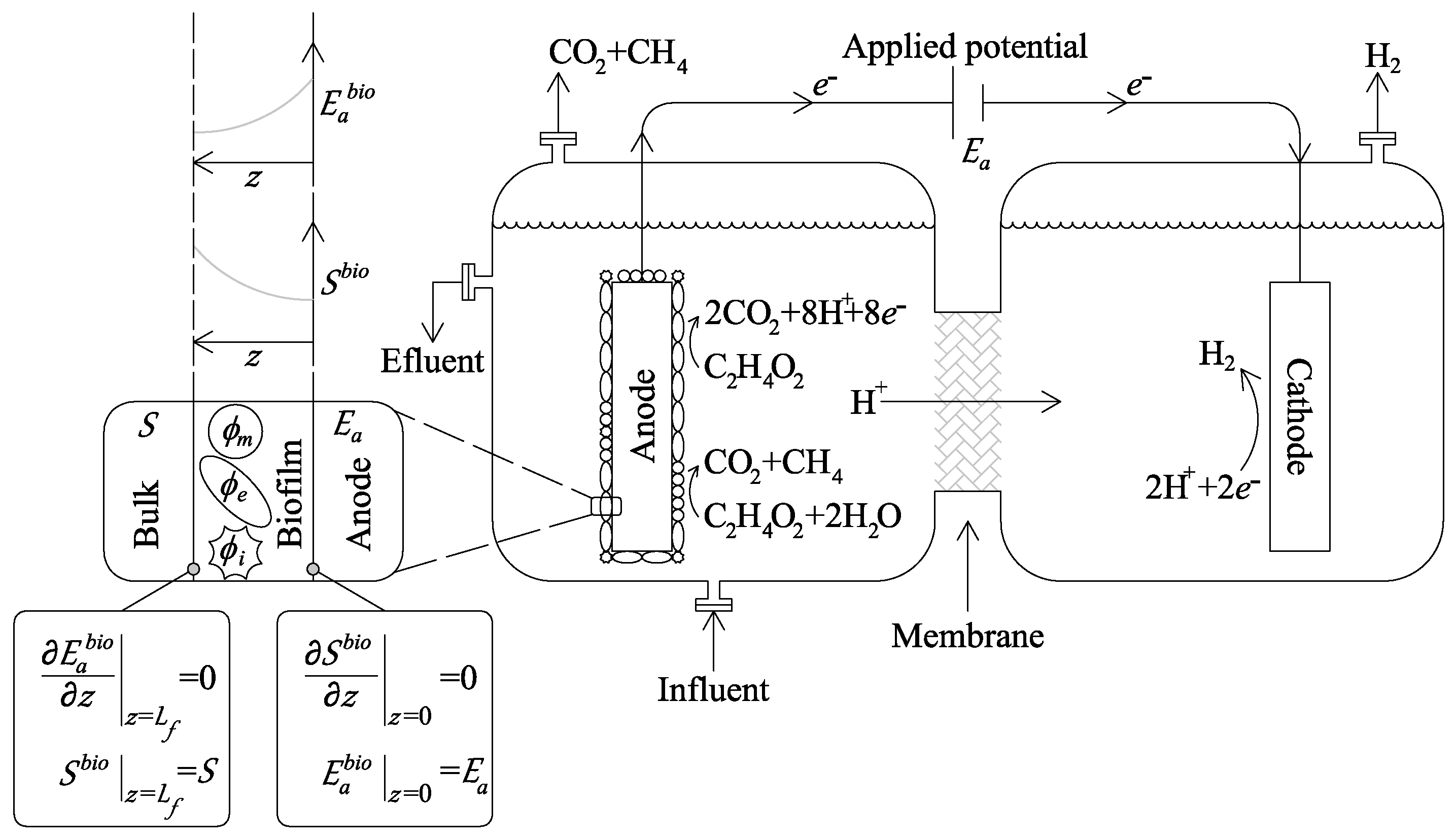
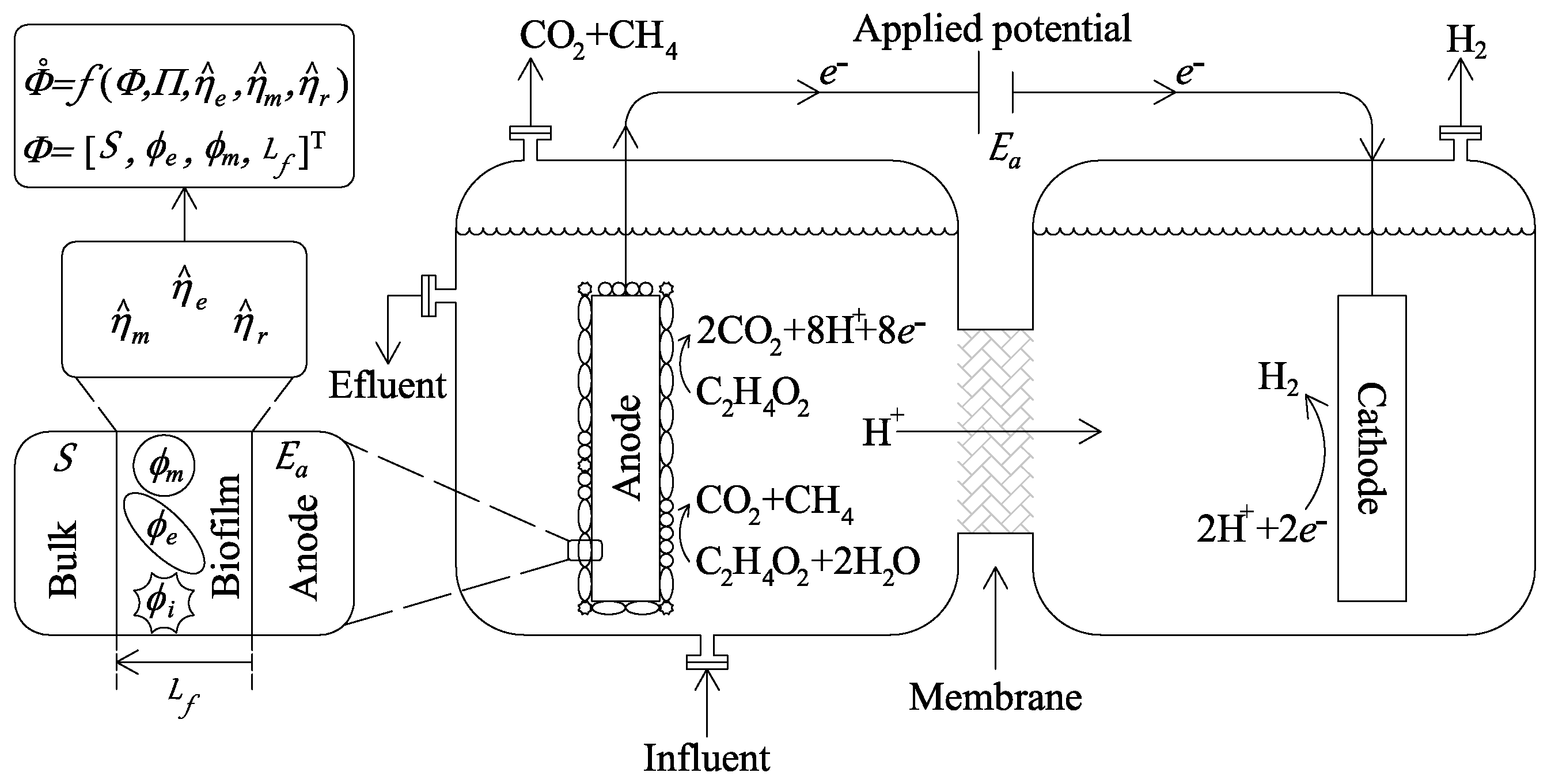
According to [26], the biofilm model is based on a set of two PDEs which are coupled to four ODEs. The model (2PDE+4ODE) is depicted in Figure 1. The following assumptions are considered for the two PDEs: (i) the biofilm is a continuum and it is homogeneous; (ii) acetic acid (C₂H₄O₂) is the only substrate; (iii) competition between methanogenic and exoelectrogenic microorganisms for the carbon source is the only one that occurs, while an inert fraction does not consume substrate; (iv) substrate and potential gradients only take place in the biofilm through the z axis, and thus, axial diffusion, as well as back diffusion, are negligible; (v) substrate is transferred by diffusion only (Fick’s law); (vi) the distribution of the substrate in the biofilm rapidly reaches a steady state once the concentration of substrate in the liquid phase changes; (vii) the distribution of the potential in the biofilm rapidly reaches a steady state once the applied potential in the anode changes; and (viii) physical and transport parameters are constant (i.e., density, conductivity, and effective diffusion).

Under these assumptions, the first PDE describes the substrate dynamics in the biofilm as follows [26]:

$$D_e\frac{{\partial }^2{S}^{bio}}{\partial z^2}-{\rho }_x\left. [{\mu }_m\left(S^{bio}\right){\varphi }_m+{\mu }_e\left(S^{bio},E_a^{bio}\right){\varphi }_e\right]=0$$

(1)

with boundary conditions:

$${\left.\frac{\partial S^{bio}}{\partial z}\right|}_{z=0}=0;S^{bio}{|}_{z=L_f}=S$$

where $S^{bio}$ and $E_a^{bio}$ are the local substrate concentration and the local potential through the biofilm, respectively, S is the substrate concentration in the liquid phase, ${\rho }_x$ is the biofilm density, $D_e$ is the effective diffusion of the substrate in the biofilm, ${\varphi }_m$ and ${\varphi }_e$ are the mass fractions of the exoelectrogenic and methanogenic microorganisms, respectively, and ${\varphi }_i$ is an inert fraction (${\varphi }_m+{\varphi }_e+{\varphi }_i$ = 1). Notice that the first boundary condition in (1) implies no substrate diffusion across the anode electrode interface. The second boundary condition corresponds to no substrate concentration gradient at the interface between the liquid phase and the biofilm surface.

Again, under the former assumptions, the second PDE describes the potential variation $E_a^{bio}$ through the biofilm [26]:

$${\kappa }_{bio}\frac{{\partial }^2{E}_a^{bio}}{\partial z^2}-\frac{\mathfrak{F}}{\gamma }\left. [k_5{\mu }_e\left(S^{bio},E_a^{bio}\right)+k_6{r}_{res}\left(E_a^{bio}\right)\right]{\rho }_x{\varphi }_e=0$$

(2)

with boundary conditions:

$${\left.\frac{\partial E_a^{bio}}{\partial z}\right|}_{z=L_f}=0;E_a^{bio}{|}_{z=0}=E_a$$

where $E_a$ is the potential at the anode surface, ${\kappa }_{bio}$ is the biofilm conductivity that can be seen as the sum of the effects related to the electron transfer mechanisms, $\mathfrak{F}$ is the Faraday constant, and $\gamma$ is the conversion time factor. Notice that the first boundary condition in (2) corresponds to no potential losses at the interface between the anode and biofilm surfaces. In contrast, the second boundary condition implies that electrons conduct only on the biofilm matrix.

Due to the mass and charge transfer, active microorganisms in the biofilm are exposed to different substrate concentrations and potentials. Therefore, their growth and oxidation rates depend on their positions inside the biofilm. The reaction rates (i.e., specific growth rates and respiration rate) in the biofilm for exoelectrogenic and methanogenic microorganisms are [26]:

$${\mu }_m\left(S^{bio}\right)={\mu }_{m,max}\frac{S^{bio}}{S^{bio}+K_{S,a}+\frac{{\left(S^{bio}\right)}^2}{K_I}}$$

(3)

$${\mu }_e\left(S^{bio},E_a^{bio}\right)={\mu }_{e,max}\frac{S^{bio}}{S^{bio}+K_{S,e}}\frac{1}{1+exp\{-\frac{\mathfrak{F}}{RT}(E_a^{bio}-E_{K_A})\}}$$

(4)

$$r_{res}\left(E_a^{bio}\right)=b_{res}\frac{1}{1+exp\{-\frac{\mathfrak{F}}{RT}(E_a^{bio}-E_{K_A})\}}$$

(5)

To find the average reaction rates, the previous expressions are integrated along the biofilm as follows [26]:

$${\overline{\mu }}_m\left(S^{bio}\right)=\frac{1}{L_f}{\int }_0^{L_f}{\mu }_m\left(S^{bio}\right)dz$$

(6)

$${\overline{\mu }}_e(S^{bio},E_a^{bio})=\frac{1}{L_f}{\int }_0^{L_f}{\mu }_e(S^{bio},E_a^{bio})dz$$

(7)

$${\overline{r}}_{res}\left(E_a^{bio}\right)=\frac{1}{L_f}{\int }_0^{L_f}{r}_{res}\left(E_a^{bio}\right)dz$$

(8)

Global Balance

The time-dependent mass balance is also based on a previous work [26] and describes an MEC system consisting in an ideal continuous stirred-tank reactor with two chambers.

$$\frac{dS}{dt}=\frac{F}{V_a}[S^{in}-S]-\frac{A_a}{V_a}[{\overline{\mu }}_m\left(S^{bio}\right)L_f{\rho }_x{\varphi }_m+{\overline{\mu }}_e(S^{bio},E_a^{bio})L_f{\rho }_x{\varphi }_e]$$

(9)

$$\frac{d{L}_f}{dt}=k_1{\overline{\mu }}_a\left(S^{bio}\right)L_f{\varphi }_m+k_4{\overline{\mu }}_e(S^{bio},E_a^{bio})L_f{\varphi }_e-b_{det}{L}_f^2-{\overline{r}}_{res}\left(E_a^{bio}\right)L_f{\varphi }_e$$

(10)

$$\frac{d{\varphi }_m}{dt}=k_1{\overline{\mu }}_m\left(S^{bio}\right)[{\varphi }_m-{\varphi }_m^2]-b_{in}{\varphi }_m-k_4{\overline{\mu }}_e(S^{bio},E_a^{bio}){\varphi }_e{\varphi }_m+{\overline{r}}_{res}{\varphi }_e{\varphi }_m$$

(11)

$$\frac{d{\varphi }_e}{dt}=[k_4{\overline{\mu }}_e(S^{bio},E_m^{bio})-{\overline{r}}_{res}\left(E_m^{bio}\right)][{\varphi }_e-{\varphi }_e^2]-b_{in}{\varphi }_e-k_1{\overline{\mu }}_m\left(S^{bio}\right){\varphi }_m{\varphi }_e$$

(12)

where S is the acetic acid concentration (as the only carbon source), $L_f$ is the biofilm thickness, F is the volumetric flow, $V_a$ is the anode chamber volume, $S_{in}$ is the inlet acetate concentration, $A_a$ is the anode active area, and $k_i$ for $i=1,2,3,4$ are yield coefficients. Under the assumption that all the generated electrons go to the anode, the expected current I (mA) is [26]:

$$I=\frac{\mathfrak{F}}{\gamma }{A}_a[k_5{\overline{\mu }}_e(S,E_a)+k_6{\overline{r}}_{res}\left(E_a\right)]L_f{\rho }_x{\varphi }_e$$

(13)

where $k_5$ and $k_6$ are yield coefficients. Then, the biofilm model consists of two PDEs (1)–(2), local reaction rates (3)–(5), average reaction rates (6)–(8), the global balance (9)–(12), and the expected current (13).

Table 3. Set of parameters.

Symbol	Description	Value	Unit	Reference
$\mathfrak{F}$	Faraday constant	96,487	C mol e${}^{-1}$	[45]
R	Ideal gas constant	8.314	atm L mol${}^{-1}$ k${}^{-1}$	[45]
${\mu }_{m,max}$	Maximum methanogenic growth rate	$0.198$	mmol S mg VS${}_a^{-1}$d${}^{-1}$	[29]
$K_{S,m}$	Half-rate constant of methanogenic	9.28 $\times {10}^{-3}$	mmol S mL${}^{-1}$	[29]
$K_I$	Inhibition constant associated with S	0.256	mmol S mL${}^{-1}$	[29]
${\mu }_{e,max}$	Maximum electricigenic growth rate	0.132	mmol S mg VS${}^{-1}$d${}^{-1}$	[29]
$K_{S,e}$	Half-rate constant of electricigenic	3 × 10${}^{-5}$	mmol S mL${}^{-1}$	[29]
$E_{K_A}$	Half maximum rate potential	−0.156	V	[46]
$b_{in}$	Inactivation constant	$0.1$	d${}^{-1}$	[46]
$b_{res}$	Endogenous respiration reaction rate	$0.05$	d${}^{-1}$	[46]
$b_{det}$	Detachment constant	60	cm${}^{-1}$ d${}^{-1}$	assumed
$D_e$	Diffusion coefficient	$0.753$	cm${}^{-2}$ d${}^{-1}$	[46]
$\gamma$	Biofilm retention constant	86,400	s d${}^{-1}$	estimated
$k_{bio}$	Biofilm conductivity	$1\times {10}^{-3}$	mA V${}^{-1}$ cm${}^{-1}$	[46]
${ϵ}_{cat}$	Efficiency of the cathode	$0.9$	dimensionless	assumed
$k_{H_2}$	Electrons transferred per mol	$0.5$	mmol H${}_2$ mEQ${}^{-1}$	assumed
$f_{exp}$	Fraction of energy-generating electrons	$0.8$	dimensionless	assumed
${\rho }_x$	Biofilm density	1042	mg VS cm${}^{-3}$	[47]
$k_1$	Yield coefficient	$0.72$	mmol CH${}_4$ mmol $S^{-1}$	[48]
$k_2$	Yield coefficient	$0.602$	mmol CO${}_2$ mmol $S^{-1}$	[48]
$k_3$	Yield coefficient	$1.366$	mmol CO${}_2$ mmol $S^{-1}$	estimated
$k_4$	Yield coefficient	$13.7$	mg VS${}_e$ mmol $S^{-1}$	[48]
$k_5$	Yield coefficient	$6.4$	mEQ mmol $S^{-1}$	estimated
$k_6$	Yield coefficient	$0.177$	mEQ mg VS${}_e^{-1}$	[46]

shows the parameters. For details, the reader is invited to refer to [26].

To solve numerically the previously reported model in (1)–(13), the numerical method ode15s in MATLAB${}^{\circledR }$ (MathWorks${}^{\mathrm{TM}}$, Natick, MA, USA) was used. The discretization of Equations (1) and (2) was firstly proposed and due to their boundary conditions, a double boundary problem was solved with the numerical method bvp5c in MATLAB${}^{\circledR }$. Simultaneously, local reaction rates (3)–(5) were obtained. Then, average reaction rates were calculated as indicated in Equations (6)–(8). Finally, the global mass balance (9)–(12) was solved and the current (13) was calculated. The entire procedure was repeated for each time step.

3. Effectiveness Factor for an MEC Biofilm

The study of reaction-diffusion phenomena in a heterogeneous reaction system commonly involves the solution of PDEs for catalyst particles, where the concept of the effectiveness factor (EF), $\eta$, is used as an alternative for avoiding the inherent computationally expensive efforts. The main idea is to express the reaction rate in a catalyst particle as a function of $\eta$. For biofilm systems, $\eta$ has been reported for zero-order and first-order kinetics [41] or Monod- [44] and Michaelis-Menten-type kinetics [40]. For more complex kinetics, there is no analytical solution.

The effectiveness factor has been defined as: the ratio of the actual reaction rate to that which would be observed if the total surface area throughout the catalyst interior were exposed to a fluid at the same conditions as those prevailing at the outside surface of the particle [33,34]. Effectiveness factors can be defined for methanogenic and exoelectrogenic microorganisms and for the respiration process as follows:

$${\eta }_m=\frac{{\overline{\mu }}_m\left(S^{bio}\right)}{{\mu }_m\left(S\right)}=\frac{\frac{1}{L_f}{\int }_0^{L_f}{\mu }_m\left(S^{bio}\right)dz}{{\mu }_{m,max}\frac{S}{S+K_{S,a}+\frac{S^2}{K_I}}}$$

(14)

$${\eta }_e=\frac{{\overline{\mu }}_e(S^{bio},E_a^{bio})}{{\mu }_e(S,E_a)}=\frac{\frac{1}{L_f}{\int }_0^{L_f}{\mu }_e(S^{bio},E_a^{bio})dz}{{\mu }_{e,max}\frac{S}{S+K_{S,e}}\frac{1}{1+exp\{-\frac{\mathfrak{F}}{RT}(E_a-E_{K_A})\}}}$$

(15)

$${\eta }_r=\frac{{\overline{r}}_{res}\left(E_a^{bio}\right)}{r_{res}\left(E_a\right)}=\frac{\frac{1}{L_f}{\int }_0^{L_f}{r}_{res}\left(E_a^{bio}\right)dz}{b_{res}\frac{1}{1+exp\{-\frac{\mathfrak{F}}{RT}(E_a-E_{K_A})\}}}$$

(16)

where $S^{bio}$ is the local substrate concentration (1), S is the bulk substrate concentration (9), $E_a^{bio}$ is the local potential (2), and $E_a$ is the anode applied potential (operating condition).

4. Numerical Implementation

To obtain the numerical values of the effectiveness factors (14)–(16), a set of operating conditions for initial substrate concentration ($S(t=0)$), inlet substrate concentration ($S_{in}$), and anode potential ($E_a$) were established to simulate the dynamical model in (9)–(12). Notice that the selected operating conditions for $S_{in}$ and $E_a$ have been reported in MEC experimental implementations [49,50,51].

Table 4. Set of operating conditions and initial condition.

Symbol	Description	Value	Unit
$S(t=0)$	Substrate initial condition	2, 3, 4, 5	g L${}^{-1}$
$S_{in}$	Substrate inlet concentration	2, 3, 4, 5	g L${}^{-1}$
$E_a$	Voltage applied	0.3, 0.4, 0.5, 0.6, 0.7, 0.8	V
T	Temperature	303	K
$V_a$	Anodic compartment volume	200	mL
F	Incoming flow	200	mL d${}^{-1}$
$A_a$	Anodic active area	30.0	cm${}^2$
$L_{f,0}$	Biofilm thickness initial condition	10	$\mathsf{\mu }$m

summarizes the operating conditions used for the numerical implementation. Volume, inlet flow, and active anode area were considered constant.

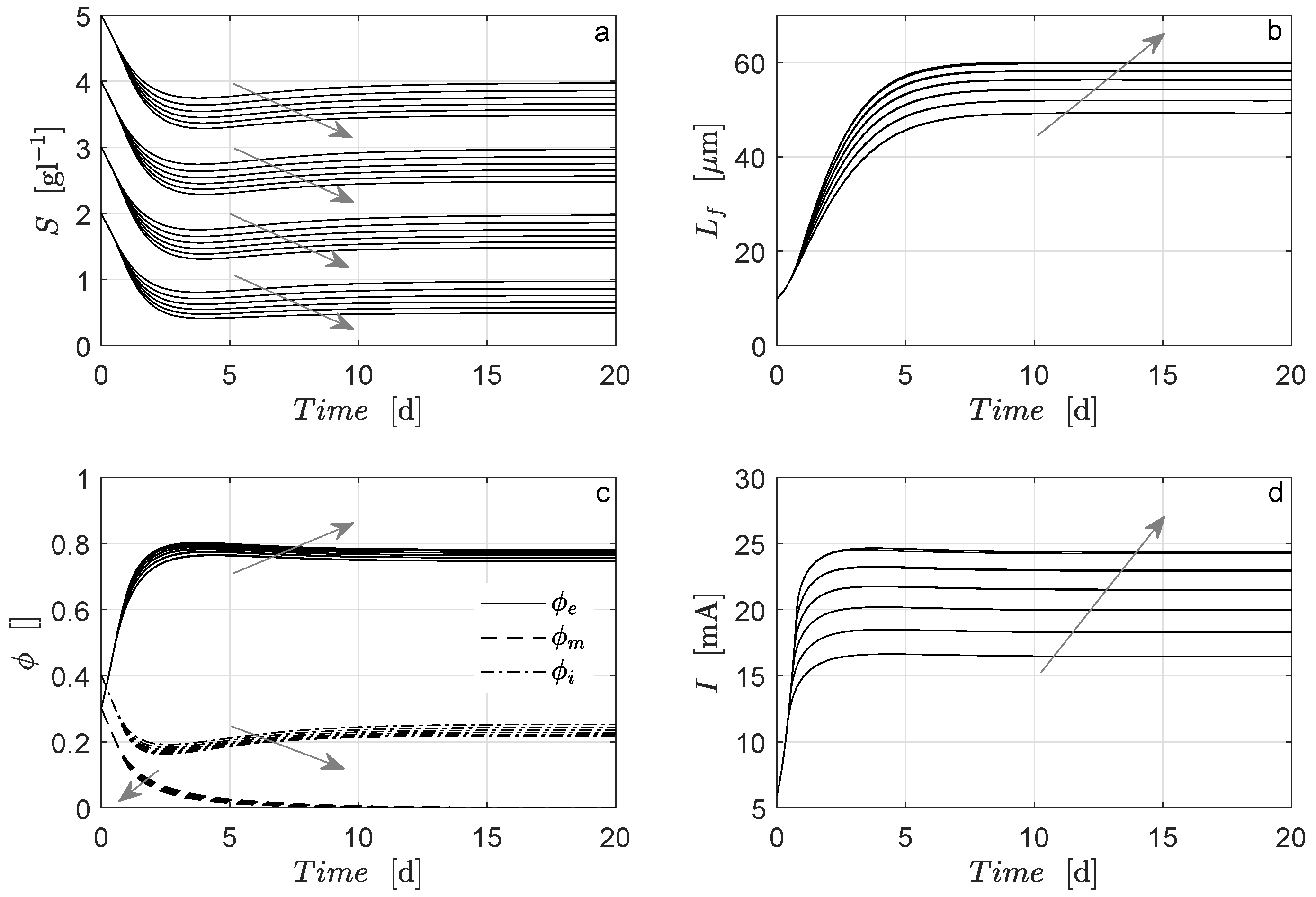
Figure 2 shows the solution of the dynamical model in (1)–(12) and the current production for different values of operating conditions (see Table 4). From the comparison of substrate profiles (Figure 2a), it can be said that a more significant consumption of substrate is obtained when higher voltage is applied. In addition, bigger values of biofilm thickness (Figure 2b), exoelectrogenic microorganism fraction (Figure 2c), and current (Figure 2d) are obtained when higher voltage is applied. In contrast, smaller values are obtained for the mass fraction of methanogenic microorganisms (Figure 2c) when higher voltages are applied.

The mass fraction of methanogenic microorganisms is zero at steady state (Figure 2c) in all numerical simulations. For the operating conditions (see Table 4), only exoelectrogenic microorganisms survive. The MEC model in (1)–(12) predicts the noncoexistence of microbial species in biofilm, although an inert fraction remains at steady state. The coexistence of MEC microbial species has been discussed in [24].

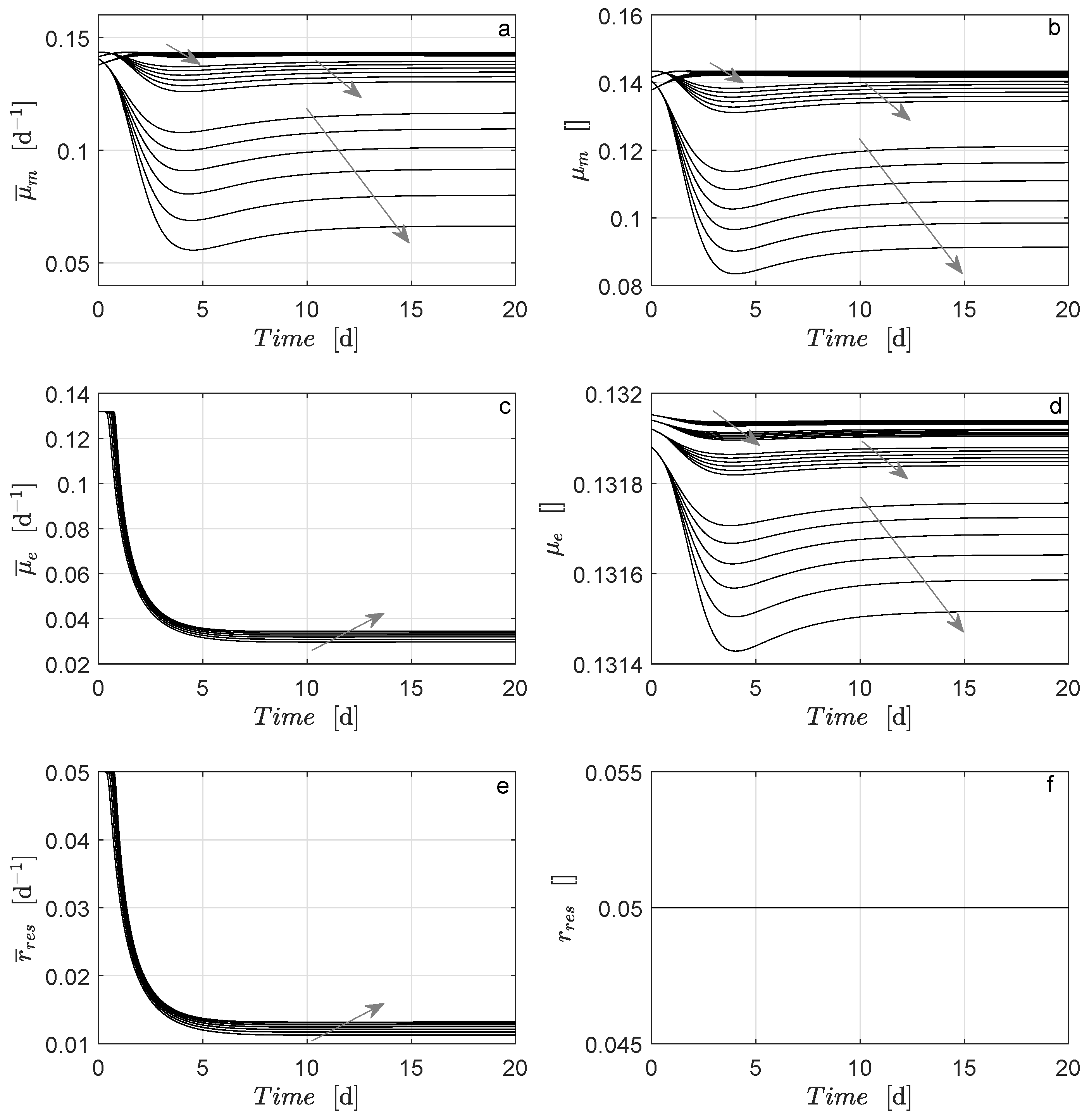
The numerical evaluation of the average reaction rates (6)–(8) and reaction rates are shown in Figure 3. It can be seen that the average reaction rate ${\overline{\mu }}_m$ (6) and reaction rate ${\mu }_m$ (Figure 3a,b, respectively) exhibit similar dynamical behavior. That is mainly due to the average reaction rate of methanogenic microorganisms being affected by the diffusional resistance offered by the biofilm; thus, ${\overline{\mu }}_m$ < ${\mu }_m$, which is expected. However, this effect is almost negligible under saturated conditions (i.e., high concentrations).

Nevertheless, the average reaction rate ${\overline{\mu }}_e$ (7) and reaction rate ${\mu }_e$ exhibit significantly different dynamical behavior. That is mainly due to the average reaction rate of exoelectrogenic microorganisms being affected by diffusional resistance in the biofilm and by the local potential. Notice that ${\mu }_e$ presents similar dynamical behavior as ${\mu }_m$ in the sense of lower magnitude in reaction rates being developed under lower bulk substrate concentration (S) and low applied voltage (V) as well, which is expected too. The average reaction rate ${\overline{r}}_{res}$ (8) and reaction rate $r_{res}$ exhibit different dynamical behavior due to the dependence of the local potential, i.e., $r_{res}$ is only a function of the applied potential, which, for this numerical implementation, is constant (see Table 4).

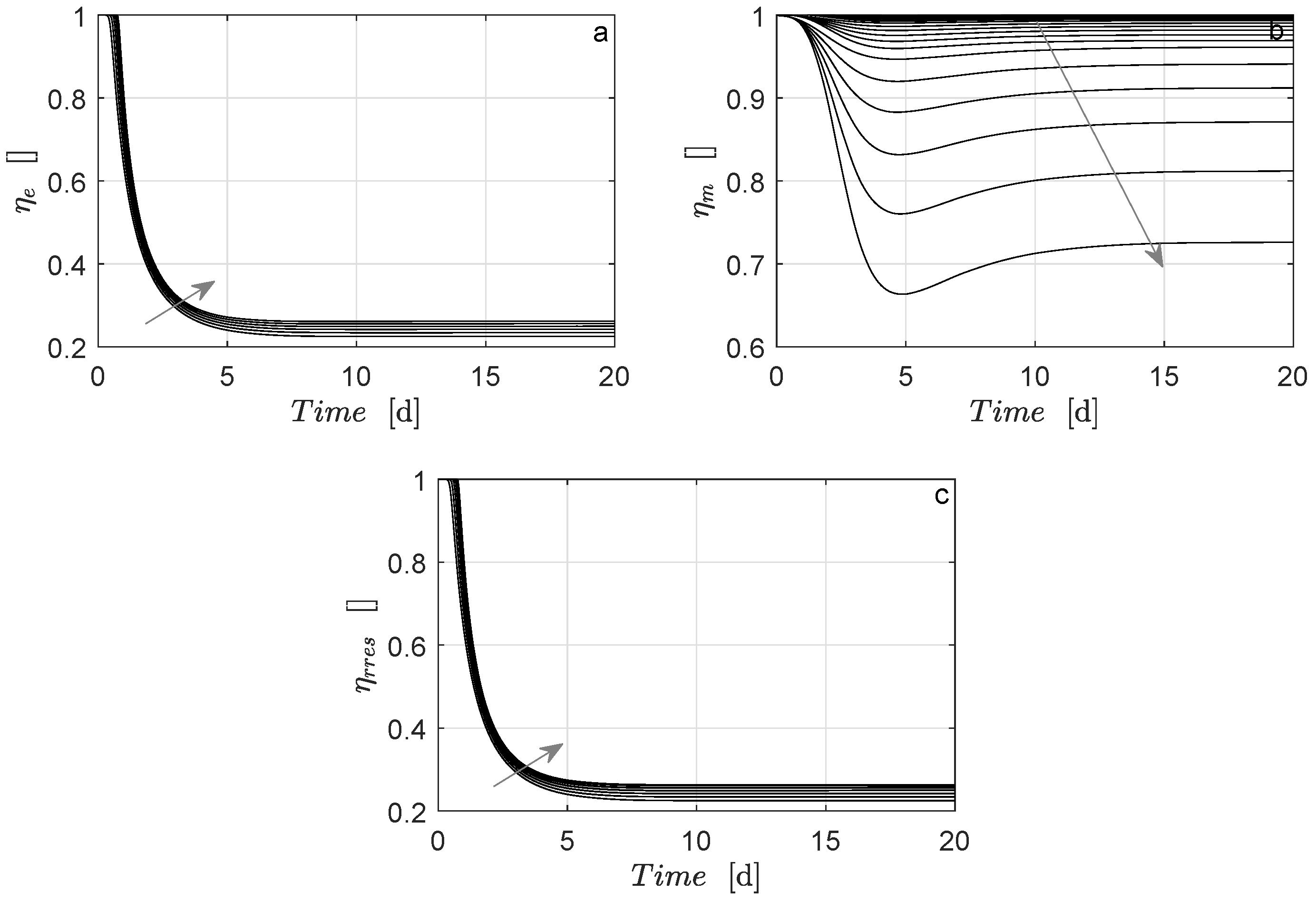
Figure 4a,c clearly show similar results for effectiveness factors ${\eta }_e$ and ${\eta }_r$. In addition, the behavior of ${\eta }_e$ and ${\eta }_r$ are in good agreement with those obtained for ${\overline{\mu }}_e$ and ${\overline{r}}_{res}$ (Figure 3c,e), respectively. These results indicate that the dominant phenomenon is conductivity (which is related to the local potential) upon mass transfer. In support information, an additional numerical case is explored when the diffusional resistance offered by biofilm is almost negligible.

It is important to point out that, as mentioned before, ${\overline{\mu }}_m$ and ${\mu }_m$ are not a function of the potential. Therefore, the effectiveness factor ${\eta }_m$ approximates unity to the extent that the saturating substrate operating conditions hold. It is essential to notice that from a practical point of view, it is convenient to operate in such conditions to remove as much substrate as possible, avoiding mass transfer limitations. On the other hand, despite mass transfer limitations not being shown for methanogenic microorganisms, for all numerical simulations of operation conditions (see Table 4), the fraction ${\varphi }_m$ is zero at steady state. Interestingly, the coexistence of microorganisms does not depend on mass transfer limitations.

From Figure 4 (at steady state), the lower and upper bounds ${\eta }_{lb}$ and ${\eta }_{ub}$ represent the permissible range for the effectiveness factors (14)–(16) for a set of parameters and operating conditions. In the present example (data in Table 3 and Table 4), these bounds result in ${\eta }_e$ = ${\eta }_{rres}$ = (0.225, 0.260) and ${\eta }_m$ = (0.725, 1).

5. Dynamical Reduced Model

The effectiveness factor for an MEC biofilm can be defined as an uncertain but bounded parameter $\widehat{{\eta }_i}\in [{\eta }_{lb,i},{\eta }_{ub,i}]$ with $i=e,m,r$. The bounded values are ${\eta }_{lb,i}=min\left({\eta }_i^{*}\right)$ and ${\eta }_{ub,i}=max\left({\eta }_i^{*}\right)$, where * stands for the value of ${\eta }_i$ obtained at steady state from the numerical evaluation of different operating conditions (see Table 4). Without loss of generality, a nominal effectiveness factor can be defined as the average of range-bounded values at steady state [52]. Therefore, the effectiveness factor for an MEC biofilm is redefined as a function of the nominal value as follows: ${\widehat{\eta }}_i={\widehat{\eta }}_{nom,i}(1+|{\Delta }_i|/100)$, where ${\Delta }_i$ is the maximum percentage of variation between the nominal value ${\widehat{\eta }}_{nom,i}$ and the upper or lower value at steady state. The values of ${\eta }_{lb,i}$, ${\eta }_{ub,i}$, ${\widehat{\eta }}_{ub,i}$, and $|{\Delta }_i|$ are obtained from Figure 4 at steady state and are shown in

Table 5. Values of effectiveness factor for a microbial electrolysis cell biofilm.

Symbol	${\widehat{\mathit{\eta }}}_{\mathit{lb},\mathit{i}}$	${\widehat{\mathit{\eta }}}_{\mathit{ub},\mathit{i}}$	${\widehat{\mathit{\eta }}}_{\mathit{nom},\mathit{i}}$	$|{\mathsf{\Delta }}_{\mathit{i}}|$
exoelectrogenic microorganisms	0.225	0.260	0.242	7.21
methanogenic microorganisms	0.725	0.999	0.857	15.4
respiration processes	0.225	0.260	0.242	7.21

.

Then, a reduction of the MEC model in (1)–(12) is then defined by the following set of ODEs:

$$\frac{dS}{dt}=\frac{F}{V_a}[S^{in}-S]-\frac{A_a}{V_a}[{\widehat{\eta }}_m{\mu }_m\left(S\right)L_f{\rho }_x{\varphi }_m+{\widehat{\eta }}_e{\mu }_e(S,E_a)L_f{\rho }_x{\varphi }_e]$$

(17)

$$\frac{d{L}_f}{dt}=k_1{\widehat{\eta }}_m{\mu }_m\left(S\right)L_f{\varphi }_m+k_4{\widehat{\eta }}_e{\mu }_e(S,E_a)L_f{\varphi }_e-b_{det}{L}_f^2-{\widehat{\eta }}_r{r}_{res}\left(E_a\right)L_f{\varphi }_e$$

(18)

$$\frac{d{\varphi }_m}{dt}=k_1{\widehat{\eta }}_m{\mu }_m\left(S\right)[{\varphi }_m-{\varphi }_m^2]-b_{in}{\varphi }_m-k_4{\widehat{\eta }}_e{\mu }_e(S,E_a){\varphi }_e{\varphi }_m+{\widehat{\eta }}_r{r}_{res}\left(E_a\right){\varphi }_e{\varphi }_m$$

(19)

$$\frac{d{\varphi }_e}{dt}=[k_4{\widehat{\eta }}_e{\mu }_e(S,E_a)-{\widehat{\eta }}_r{r}_{res}\left(E_a\right)][{\varphi }_e-{\varphi }_e^2]-b_{in}{\varphi }_e-k_1{\widehat{\eta }}_m{\mu }_m\left(S\right){\varphi }_m{\varphi }_e$$

(20)

Consequently, the dynamic MEC model in (1)–(12) with the biofilm model described by the set of PDEs (1)–(2) and the set of ODEs (9)–(12) is reduced through an effectiveness factor for an MEC biofilm. The reduced MEC model, in a compact form, is defined as follows:

$${\displaystyle \dot{\mathsf{\Phi }}=f(\mathsf{\Phi },\Pi ,{\widehat{\eta }}_e,{\widehat{\eta }}_m,{\widehat{\eta }}_r),\mathsf{\Phi }\left(t_0\right)={\mathsf{\Phi }}_0}$$

(21)

It consists of the set of ODEs (17)–(20); state variables $\mathsf{\Phi }=[S,L_f,{\varphi }_e,{\varphi }_m]$${}^T$; the set of parameters $\Pi =[$${\mu }_{max,e}$, ${\mu }_{max,m}$, $K_{S,e}$, $K_{S,m}$, $K_i$, $E{k}_a$, ${\rho }_X$, $b_{det}$, $b_{res}$, $b_{in}$, $f_{exp}$, $D_e$, $k_{bio}$, $k_1$, $k_2$, $k_3$, $k_4$, $k_5$, $k_6$, $e_{cat}$, $k_{H2}]$; and operational conditions $[S_{in}$, $E_a$, T, $V_a$, F, $A_a]$ with uncertain but bounded parameters ${\widehat{\eta }}_e$, ${\widehat{\eta }}_m$, and ${\widehat{\eta }}_r$, where ${\widehat{\eta }}_e={\widehat{\eta }}_{nom,e}(1+|{\Delta }_e|/100)$, ${\widehat{\eta }}_m={\widehat{\eta }}_{nom,m}(1+|{\Delta }_m|/100)$, and ${\widehat{\eta }}_r={\widehat{\eta }}_{nom,r}(1+|{\Delta }_r|/100)$.

The main assumptions of the reduced ODE MEC model are the following: (i) acetate is the only substrate in the feed wastewater; (ii) the anodic chamber operates as an ideal continuous stirred-tank reactor; (iii) all variables are considered spatially uniform; (iv) exoelectrogenic and (possibly) methanogenic microbial populations are mostly attached to the anodic biological biofilm; (v) in consequence, biomass growth in the anodic bulk phase is negligible; (vi) microbial populations compete for the same substrate; (vii) there is instant gas transfer from the liquid to the gas phase; and (viii) pH = 5.5 and temperature T = 25 °C are constant. Figure 5 shows the schematic representation of the reduced ODE MEC model in (21).

It is important to remark that even when suspended bacteria may affect biofilm growth, mass transfer, and electricity generation in BES [53,54], the former assumptions (physically plausible) imply the inhibition of methanogenic archaea growth (mainly because of the acid pH) and favor that the only exoelectrogenic bacteria that survive are eventually attached to the anode [55].

Experimental results in the literature reported that there are lower efficiency and electricity generation when scaling up BES [3,6]. The reactor and electrode size influence the efficiency of the MEC system and therefore the electricity generation [3,6]. Despite ideal suppositions on the reduced ODE MEC model, the proposed EF approach could be applied to a more complex PDE MEC system. In this sense, a detailed PDE MEC model for current, potential, and nonideal flow patterns can be solved numerically for complex geometries and then applied to the proposed EF approach on a representative ODE MEC model. Thus, reactor-electrode size side effects on mass transfer and electricity generation could be included in the alternative reduced ODE MEC model in a scale-up approach.

5.1. Equilibrium Points

In order to recognize the possible steady-state solutions for the model in (21), it is necessary to compute the equilibrium points and then classify them in the sense of stability criteria. Then, the following steps are performed: (i) to compute an equilibrium point under parameters and operating conditions; (ii) to find the Jacobian matrix of the nonlinear reduced model in (21); (iii) to compute the eigenvalues of the Jacobian matrix at an equilibrium point; and (iv) to corroborate the criteria of stability. The equilibrium point is locally asymptotically stable if all eigenvalues have negative real parts. Otherwise, if there is even one eigenvalue with a positive real part, the equilibrium point is unstable. As an example of this procedure,

Table 6. Equilibrium points $\psi$ of reduced model in (21).

	${\mathit{S}}^{*}$ [g L${}^{-1}$]	${\mathit{L}}_{\mathit{f}}^{*}$ [$\mathsf{\mu }$m]	${\mathit{\varphi }}_{\mathit{m}}^{*}$ []	${\mathit{\varphi }}_{\mathit{e}}^{*}$ []	PM/NPM	SP/NSP
${\psi }_{01}$	0.654	56.393	0	0.772	PM	SP
${\psi }_{02}$	−0.012	69.138	0	0.805	NPM	SP
${\psi }_{03}$	2	0	0	0.0	PM	NSP
${\psi }_{04}$	2	0	0	0.772	NPM	NSP
${\psi }_{05}$	2	0	−0.008	0.0	NPM	NSP
${\psi }_{06}$	2	0	−4.508	1.016	NPM	NSP
${\psi }_{07}$	2	−0.138	−0.008	0	NPM	NSP
${\psi }_{08}$	0.01856	−15.92	−21.21	0	NPM	NSP
${\psi }_{09}$	−2.013	22.65	0.5761	0	NPM	NSP
${\psi }_{10}$	−7.129	34.16	0.6721	0	NPM	NSP
${\psi }_{11}$	−23.8	−57.43	1.409	0	NPM	NSP
${\psi }_{12}$	0.00005	−16.54	0	−133.2	NPM	NSP
${\psi }_{13}$	−0.00073	−71.14	0	1.306	NPM	NSP

PM = physical meaning, NPM = nonphysical meaning, SP = stable point, NSP = non stable point, * stands for steady state.

shows the numerical evaluation of the equilibrium points under the set of parameters in Table 3 and operating conditions $S(t=0)$ = 2 [g L${}^{-1}$], $S_{in}=$ 2 [g L${}^{-1}$], and $E_a=$ 0.3 [V], and the remaining operating conditions are shown in Table 4.

Notice that only the equilibrium point ${\psi }_{01}$ exhibits stable behavior and has a physical meaning. It is said that the MEC system is operating in a desirable condition of noncoexistence of microorganisms in which only exoelectrogenic microorganisms degrade the substrate [24]. Equilibrium point ${\psi }_{02}$ exhibits stable behavior, but this point does not have physical meaning because this would imply a physically impossible negative value for the substrate at steady state. Equilibrium point ${\psi }_{03}$ is particularly interesting because it shows that the MEC system exhibits washout and that the steady-state substrate concentration is given by its inlet composition. However, ${\psi }_{03}$ will not arise because it is an unstable equilibrium point. The analysis is similar for the other equilibrium points ${\psi }_{04}$ to ${\psi }_{13}$, from which it can be deduced that the reduced MEC model in (21) has only one reachable locally stable equilibrium point ${\psi }_{01}$ under the set of parameters $\Pi$ (Table 3) and the operating conditions under consideration for this example.

5.2. Parametric Sensitivity Analysis

Departing from the reduced MEC model in (21), a sensitivity parametric analysis [52] is performed to determine which parameters in $\mathsf{\Pi }$ affect the dynamical behavior of the field $f(\mathsf{\Phi };\pi )$. For a set of parameters $\pi$, the approximate solution for the sensitivity function is computed by the simultaneous solution of the MEC model in (21) and the linear time-varying sensitivity equation ${\dot{\mathsf{\Theta }}}_f$ as follows [52]:

$$\begin{array}{c}{\displaystyle \dot{\mathsf{\Phi }}=f(\mathsf{\Phi },{\pi }_0),\mathsf{\Phi }\left(t_0\right)={\mathsf{\Phi }}_0}\hfill \\ {\displaystyle {\dot{\mathsf{\Theta }}}_f={\left. [\frac{\mathsf{\partial }f(\mathsf{\Phi },\mathsf{\Pi })}{\mathsf{\partial }\mathsf{\Phi }}\right]}_{{\pi }_0}{\mathsf{\Theta }}_f+{\left. [\frac{\mathsf{\partial }f(\mathsf{\Phi },\mathsf{\Pi })}{\mathsf{\partial }\mathsf{\Pi }}\right]}_{{\pi }_0},{\mathsf{\Theta }}_f\left(t_0\right)=0}\hfill \end{array}$$

(22)

The parameters of Table 3 and operation conditions in Table 4 are used to numerically solve Equation (22). In addition, in order to appreciate the parameter subset having the most significant effect of the MEC model in (21), the following parameter values are changed from Table 4: $S_{in}=1$ [g L${}^{-1}$], $E_a=0.3$ [V], and $A_a=5$ [cm${}^2$]. The following values for the effectiveness factor for an MEC biofilm are considered: ${\widehat{\eta }}_m=0.98$, ${\widehat{\eta }}_e=0.25$, and ${\widehat{\eta }}_r=0.25$. Notice that such values belong to the uncertainty value range shown in Table 5. The following initial conditions for the numerical solution of (22) are considered: $\mathsf{\Phi }\left(t_0\right)$ = [1 g L${}^{-1}$, 10 $\mathsf{\mu }$ m, 0.3, 0.3]${}^T$ and ${\mathsf{\Theta }}_0$ = [1, 1, 1, 1]${}^T$. The numerical method ode15s in MATLAB${}^{\circledR }$ was used to solve numerically Equation (22).

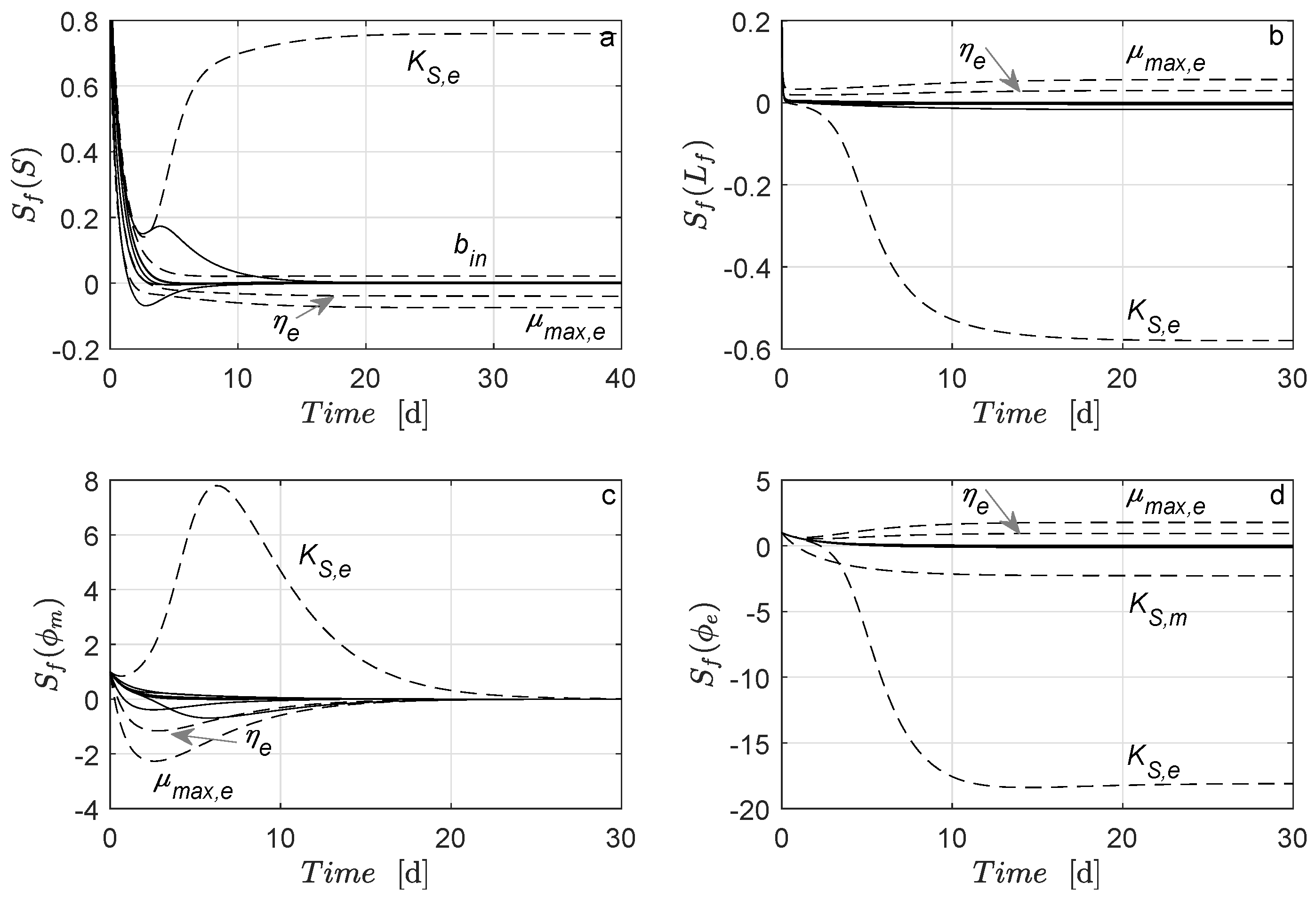
Figure 6 shows the numerical solution of (22). Notice that at stable steady-state conditions, the parameter subset having the most significant effect of the MEC model in (21) is: $K_{S,e}$, $b_{in}$, ${\mu }_{max,e}$, and ${\widehat{\eta }}_e$. Interestingly, only the effectiveness factor ${\widehat{\eta }}_e$ arises as the important parameter in the parametric sensitivity analysis in comparison to ${\widehat{\eta }}_m$ and ${\widehat{\eta }}_r$.

From Figure 6c, $K_{S,e}$, ${\widehat{\eta }}_e$, and ${\mu }_{max,e}$ arise as the important parameters in the parametric sensitivity analysis for $S_f\left({\mathsf{\Phi }}_m\right)$ under transient condition. However, all solutions of $S_f\left({\mathsf{\Phi }}_m\right)$ converge to zero at steady state. Consequently, all parameters exert a significant influence on the ${\mathsf{\Phi }}_m^{*}$ value when they change (${}^{*}$ stands for steady state).

5.3. Open-Loop Dynamical Behavior

The performance of the reduced MEC model in (21) is evaluated and compared in an open-loop simulation with the following ODE model reported by Pinto et al. [30]:

$$\begin{array}{c}\dot{S}=(S_{in}-S)D-q_e{X}_e-q_m{X}_m\hfill \\ {\dot{X}}_e={\mu }_e{X}_e-\alpha X_e\hfill \\ {\dot{X}}_m={\mu }_m{X}_m-\alpha X_m\hfill \\ {\dot{M}}_{ox}=-Y_M{q}_e+\frac{\gamma }{V_{reac}{X}_e}\frac{I_{MEC}}{m\mathfrak{F}}\hfill \end{array}$$

(23)

where S is the substrate (acetate) concentration; $X_e$ and $X_m$ are the exoelectrogenic and methanogenic microorganism concentrations, respectively; $M_{ox}$ is the oxidized mediator fraction per exoelectrogenic microorganism; $q_e$ and $q_m$ are the acetate consumption rates by exoelectrogenic and methanogenic microorganisms, respectively; ${\mu }_e$ and ${\mu }_m$ are the growth rates; $\alpha$ is the dimensionless biofilm retention constant; D is the dilution rate ($D=F_{in}{V}_{reac}^{-1}$); $Y_M$ is the oxidized mediator yield; $\gamma$ is the mediator molar mass; m is the number of electrons transferred per mol of mediator; and $\mathfrak{F}$ is the Faraday constant. The following expressions are included:

$$\begin{array}{c}{\displaystyle M_{total}=M_{red}+M_{ox}}\hfill \\ {\displaystyle q_e=q_{max,e}\frac{S}{K_{S,e}+S}\frac{M_{ox}}{K_M+M_{ox}}}\hfill \\ {\displaystyle q_m=q_{max,m}\frac{S}{K_{S,m}+S}}\hfill \\ {\displaystyle {\mu }_e={\mu }_{max,e}\frac{S}{K_{S,e}+S}\frac{M_{ox}}{K_M+M_{ox}}}\hfill \\ {\displaystyle {\mu }_m={\mu }_{max,m}\frac{S}{K_{S,m}+S}}\hfill \\ {\displaystyle \alpha =\left\{\begin{array}{cc}\frac{{\mu }_e{X}_e+{\mu }_m{X}_m}{X_e+X_m}& \mathrm{if}{X}_e+X_m>X_{max}\\ 0& \mathrm{otherwise}\end{array}\right.}\hfill \end{array}$$

(24)

where $M_{total}$ is the total mediator fraction per microorganism; $M_{red}$ is the reduced mediator fraction per exoelectrogenic microorganism; $q_{max,e}$ and $q_{max,m}$ are the maximum acetate consumption rates; ${\mu }_{max,e}$ and ${\mu }_{max,m}$ are the maximum growth rates; $K_{S,e}$ and $K_{S,m}$ are the half saturation constants; and $X_{max}$ is the maximum attainable biomass concentration.

Table 7. Set of parameters for model in (23) and auxiliary functions in (24).

Symbol	Description	Value	Unit
${\mu }_{max,e}$	Max. electricigenic growth rate	2.0	d${}^{-1}$
${\mu }_{max,m}$	Max. methanogenic growth rate	0.1	d${}^{-1}$
$q_{max,e}$	Max. electricigenic reaction rate	14.0	d${}^{-1}$
$q_{max,m}$	Max. methanogenic reaction rate	14.12	d${}^{-1}$
$Y_{CH4}$	Methane yield	0.28	ml $C{H}_4$ mL $S^{-1}$
$K_{S,e}$	Half-rate constant of electricigens	20.0	mg S L${}^{-1}$
$K_{S,m}$	Half-rate constant of methanogens	20.0	mg S L${}^{-1}$
$K_M$	Mediator half-rate constant	0.01	mg M L${}^{-1}$
$M_{total}$	Mediator fraction	0.05	mg M mg $X^{-1}$
$X_{max}$	Anode biofilm space limitation	512.5	mg X L${}^{-1}$
$R_{min}$	Lowest internal resistance	30.0	$\mathsf{\Omega }$
$R_{max}$	Highest internal resistance	2000.0	$\mathsf{\Omega }$
$K_R$	Constant	0.024	L mg $X^{-1}$
$Y_M$	Oxidized mediator yield	36.6	mg M mg $S^{-1}$
$E_{CEF}$	Counter-electromotive force	−0.35	V
$Y_{H2}$	Cathode efficiency	0.8	dimensionless
$\gamma$	Mediator molar mass	663,400	mg M mol $M^{-1}$
${\eta }_{act}$	Activation overpotential	0.05	V

summarizes the set of parameters used in the model in (23) and in the auxiliary functions (24).

Notice that the biofilm in the model in (23) is limited by $X_{max}$. Therefore, for the sake of normalization, the biomass fraction for the model in (23) is defined as follow:

$${\displaystyle {\varphi }_e=\frac{X_e}{X_{max}},{\varphi }_m=\frac{X_m}{X_{max}}}$$

(25)

The operating conditions for both models are: $S_{in}$ = 2 g L${}^{-1}$, $E_a$ = 0.5 V, $V_a$ = 50 mL, and F = 50 mL. Additional operating conditions used in the reduced model in (21) are $A_a=5$ cm${}^2$, ${\eta }_e$ = ${\eta }_r$ = 0.25, and ${\eta }_m$ = 0.95. The initial condition for the model in (23) is: [2 g L${}^{-1}$, 200 mg L${}^{-1}$, 100 mg L${}^{-1}$, 0.25 mg $M_{ox}$ mg $X^{-1}]$${}^T$. The initial condition for the model in (21) is: [2 g L${}^{-1}$, 20 $\mathsf{\mu }$m, 0.3, 0.3]${}^T$. The numerical method ode15s in MATLAB${}^{\circledR }$ was used to solve numerically the model in (21) and the model in (23)–(25).

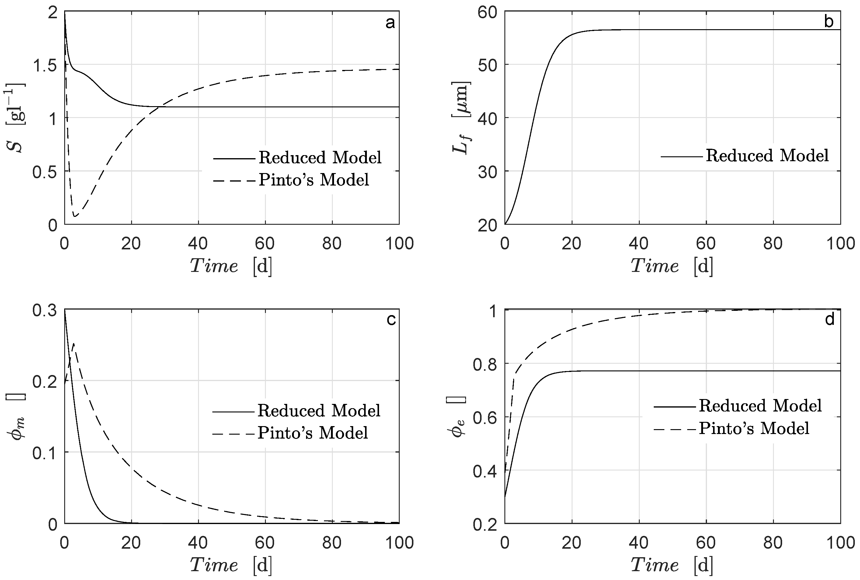
Figure 7 illustrates the dynamical behavior of the state variables of the reduced model in (21) and the model in (23). In the same figure, it can be seen that S in both models converges to a near-steady state. Notice that the values for S predicted by the model in (23) are smaller than the ones predicted by the reduced model in (21) for $0<t<20$ [d] (see Figure 7a). Moreover, the model in (23) predicts a minimum substrate concentration for $0<t<5$ [d]. This is because there is an increase in the mass fractions of methanogenic (Figure 7c) and exoelectrogenic (Figure 7d) microorganisms. In addition, for $t>5$ [d], the model in (23) predicts: (i) an increase in S (Figure 7a) and the mass fraction of exoelectrogenic microorganisms (Figure 7d) and (ii) a decrease in the mass fraction of methanogenic microorganisms. On the other hand, all the states of the reduced model in (21) exhibit smooth dynamic behavior. Moreover, states S and ${\mathsf{\Phi }}_m$ decrease, and states $L_f$ and ${\mathsf{\Phi }}_e$ slowly increase and finally reach a steady state. It should be noted that the dynamic smoothness of the reduced model in (21) may be desirable in control or real-time applications.

It is important to remark that the aim of the work was to propose a methodology to obtain an effectiveness factor for biofilm in an MEC system and use it in the reduction of the PDE biofilm MEC model to the ODE MEC model, but the experimental validation stricto sensu is not provided here. Indeed, the numerical implementation includes operating conditions from the literature [49,50,51]. Moreover, the reduced ODE model was compared with the validated model taken also from [30] and the results were in good agreement. Nevertheless, the parameters of the reduced model should be adjusted to be successfully applied to lab-scale or pilot-scale implementations. This task is planned as future work.

6. Conclusions

In this work, an effectiveness factor for the microbial electrolysis cell model was proposed. This effectiveness factor was defined for the biofilm respiration process and methanogenic and exoelectrogenic microorganisms. Departing from a partial differential equation and numerical data obtained from a set of operating conditions, a set of uncertain but bounded ranges of effectiveness factor values was obtained. The stability and parametric sensibility of the reduced model were evaluated. Then, a reduced model based on ordinary differential equations was obtained. The reduced model was analyzed in the sense of stability and parametric sensibility. The reduced model was also tested in numerical simulation using a validated model taken from the literature.

The proposed effectiveness factor was included in a microbial electrolysis cell model described by a set of ordinary differential equations. The procedure is an alternative to address the tradeoff between (i) the local description of multipopulation microorganisms, local mass, and local potential in the biofilm and (ii) a simple and reliable alternative description of biofilm in an ordinary differential equation representing a continuous microbial electrolysis cell system.

The procedure could be extended to models comprising mass and charge transport in biofilm, simulated in two or three dimensions and then coupled with global mass balances for microbial electrolysis cell systems.

References

1. Logan, B.E.; Rossi, R.; Ragab, A.; Saikaly, P.E. Electroactive microorganisms in bioelectrochemical systems. Nat. Rev. Microbiol. 2019, 17, 307–3019. [Google Scholar] [CrossRef] [PubMed]
2. Logan, B.E.; Call, D.; Cheng, S.; Hamelers, H.V.; Sleutels, T.H.; Jeremiasse, A.W.; Rozendal, R.A. Microbial electrolysis cells for high yield hydrogen gas production from organic matter. Environ. Sci. Technol. 2008, 42, 8630–8640. [Google Scholar] [CrossRef] [PubMed]
3. Leicester, D.; Amezaga, J.; Heidrich, E. Is bioelectrochemical energy production from wastewater a reality? Identifying and standardising the progress made in scaling up microbial electrolysis cells. Renew. Sustain. Energy Rev. 2020, 133, 110279. [Google Scholar] [CrossRef]
4. Mejía-López, M.; Verea, L.; Joseph Sebastian, P.; Verde, A.; Perez-Sarinana, B.Y.; Campos, J.; Hernández-Romano, J.; Moeller-Chávez, G.E.; Lastres, O.; Monjardín-Gámez, J.J. Improvement of biofilm formation for application in a single chamber microbial electrolysis cell. Fuel Cells. 2021, 21, 317–327. [Google Scholar] [CrossRef]
5. Fudge, T.; Bulmer, I.; Bowman, K.; Pathmakanthan, S.; Gambier, W.; Dehouche, Z.; Al-Salem, S.M.; Constantinou, A. Microbial Electrolysis Cells for Decentralised Wastewater Treatment: The Next Steps. Water 2021, 13, 445. [Google Scholar] [CrossRef]
6. Escapa, A.; Mateos, R.; Martínez, E.J.; Blanes, J. Microbial electrolysis cells: An emerging technology for wastewater treatment and energy recovery. From laboratory to pilot plant and beyond. Renew. Sustain. Energy Rev. 2016, 55, 942–956. [Google Scholar] [CrossRef]
7. Recio-Garrido, D.; Perrier, M.; Tartakovsky, B. Modeling, optimization and control of bioelectrochemical systems. Chem. Eng. J. 2016, 289, 180–190. [Google Scholar] [CrossRef]
8. Gadkari, S.; Gu, S.; Sadhukhan, J. Towards automated design of bioelectrochemical systems: A comprehensive review of mathematical models. Chem. Eng. J. 2018, 343, 303–316. [Google Scholar] [CrossRef]
9. Rousseau, R.; Etcheverry, L.; Roubaud, E.; Basséguy, R.; Délia, M.L.; Bergel, A. Microbial electrolysis cell (MEC): Strengths, weaknesses and research needs from electrochemical engineering standpoint. Appl. Energy. 2020, 257, 113938. [Google Scholar] [CrossRef]
10. Osman, A.I.; Deka, T.J.; Baruah, D.C.; Rooney, D.W. Critical challenges in biohydrogen production processes from the organic feedstocks. Biomass Convers. Biorefin. 2020, 1–19. [Google Scholar] [CrossRef]
11. Lewis, A.J.; Borole, A.P. Microbial electrolysis cells using complex substrates achieve high performance via continuous feeding-based control of reactor concentrations and community structure. Appl. Energy 2019, 2040, 608–616. [Google Scholar] [CrossRef]
12. Lacroix, R.; Roubaud, E.; Erable, B.; Etcheverry, L.; Bergel, A.; Basséguy, R.; Da Silva, S. Design of 3D microbial anodes for microbial electrolysis cells (MEC) fuelled by domestic wastewater. Part I: Multiphysics modelling. J. Environ. Chem. Eng. 2021, 9, 105476. [Google Scholar] [CrossRef]
13. Sewsynker, Y.; Gueguim Kana, E.B.; Lateef, A. Modelling of biohydrogen generation in microbial electrolysis cells (MECs) using a committee of artificial neural networks (ANNs). Biotechnol. Biotechnol. Equip. 2015, 29, 1208–1215. [Google Scholar] [CrossRef] [Green Version]
14. Mohd Asrul, M.A.; Farid Atan, M.; Halim Yun, H.A.; Hui Lai, J.C. Mathematical model of biohydrogen production in microbial electrolysis cell: A review. Int. J. Hydrogen Energy 2021, 46, 37174–37191. [Google Scholar] [CrossRef]
15. Hernández-García, K.M.; Cercado, B.; Rivero, E.P.; Rivera, F.F. Theoretical and experimental evaluation of the potential-current distribution and the recirculation flow rate effect in the performance of a porous electrode microbial electrolysis cell (MEC). Fuel 2020, 279, 118463. [Google Scholar] [CrossRef]
16. Zhang, X.C.; Halme, A. Modelling of a microbial fuel cell process. Biotechnol. Lett. 1995, 17, 809–814. [Google Scholar] [CrossRef]
17. Xia, C.; Zhang, D.; Pedrycz, W.; Zhu, Y.; Guo, Y. Models for Microbial Fuel Cells: A critical review. Biotechnol. Lett. 2018, 373, 119–131. [Google Scholar] [CrossRef]
18. Jadhav, A.A.; Carmona-Martínez, A.C.; Chendake, A.D.; Pandit, A.; Pant, D. Modeling and optimization strategies towards performance enhancement of microbial fuel cells. Bioresour. Technol. 2021, 320, 124256. [Google Scholar] [CrossRef]
19. Deb, D.; Patel, R.; Balas, V.E. A Review of Control-Oriented Bioelectrochemical Mathematical Models of Microbial Fuel Cells. Processes 2020, 8, 583. [Google Scholar] [CrossRef]
20. Hosseinzadeh, A.; Zhou, J.L.; Altaee, A.; Baziar, M.; Li, D. Effective modelling of hydrogen and energy recovery in microbial electrolysis cell by artificial neural network and adaptive network-based fuzzy inference system. Bioresour. Technol. 2020, 316, 123967. [Google Scholar] [CrossRef]
21. Pinto, R.P.; Srinivasan, B.; Escapa, A.; Tartakovsky, B. Multi-Population Model of a Microbial Electrolysis Cell. Environ. Sci. Technol. 2011, 45, 5039–5046. [Google Scholar] [CrossRef] [Green Version]
22. Yahya, A.M.; Hussain, M.A.; Abdul Wahab, A.K. Modeling, optimization, and control of microbial electrolysis cells in a fed-batch reactor for production of renewable biohydrogen gas. Int. J. Energy Res. 2014, 39, 557–572. [Google Scholar] [CrossRef]
23. Dudley, H.J.; Lu, L.; Ren, Z.J.; Bortz, D.M. Sensitivity and Bifurcation Analysis of a Differential-Algebraic Equation Model for a Microbial Electrolysis Cell. SIAM J. Appl. Dyn. Syst. 2019, 18, 709–728. [Google Scholar] [CrossRef]
24. Flores-Estrella, R.A.; Rodriguez-Valenzuela, G.; Ramirez-Landeros, J.R.; Alcaraz-Gonzalez, V.; Gonzalez-Alvarez, V. A simple microbial electrochemical cell model and dynamic analysis towards control design. Chem. Eng. Commun. 2019, 207, 493–505. [Google Scholar] [CrossRef]
25. Alcaraz-Gonzalez, V.; Rodriguez-Valenzuela, G.; Gomez-Martinez, J.J.; Dotto, G.L.; Flores-Estrella, R.A. Hydrogen production automatic control in continuous microbial electrolysis cells reactors used in wastewater treatment. J. Environ. Manag. 2021, 281, 111869. [Google Scholar] [CrossRef]
26. Flores-Estrella, R.A.; Garza-Rubalcava, U.J.; Haarstrick, A.; Alcaraz-Gonzalez, V. A Dynamic Biofilm Model for a Microbial Electrolysis Cell. Processes 2019, 7, 183. [Google Scholar] [CrossRef] [Green Version]
27. Reyes-Vidal, Y.; López-Maldonado, J.; Castañeda, F.; Orozco, G.; Rivera, F.F. Evaluation of Inlet Design and Flow Rate Effect on Current Density Distribution in a Microbial Electrolysis Cell Using Computational Simulation Techniques, Coupling Hydrodynamics and Bioanode Kinetics. Int. J. Chem. React. Eng. 2018, 16, 20170259. [Google Scholar] [CrossRef]
28. Hernández-García, K.M.; Cercado, B.; Rodríguez, F.A.; Rivera, F.F.; Rivero, E.P. Modeling 3D current and potential distribution in a microbial electrolysis cell with augmented anode surface and non-ideal flow pattern. Biochem. Eng. J. 2020, 162, 107714. [Google Scholar] [CrossRef]
29. Bernard, O.; Hadj-Sadok, Z.; Dochain, D.; Genovesi, A.; Steyer, J.P. Dynamical model development and parameter identification for an anaerobic wastewater treatment process. Biotechnol. Bioeng. 2000, 75, 424–438. [Google Scholar] [CrossRef]
30. Pinto, R.P.; Tartakovsky, B.; Srinivasan, B. Optimizing energy productivity of microbial electrochemical cells. J. Process Control 2012, 22, 1079–1086. [Google Scholar] [CrossRef]
31. Alcaraz-Gonzalez, V.; Rodriguez-Valenzuela, G.; Gomez-Martinez, J.J.; Dotto, G.L.; Flores-Estrella, R.A. FPGA-Based Implementation of an Optimization Algorithm to Maximize the Productivity of a Microbial Electrolysis Cell. Processes 2021, 9, 1111. [Google Scholar]
32. Álvarez-Ramirez, J.; Valdés-Parada, F.J.; Ochoa-Tapia, J.A. Low-Order Models for Catalyst Particles: A dynamic effectiveness factor approach. AICHE J. 2005, 51, 3219–3230. [Google Scholar] [CrossRef]
33. Aris, R. The Mathematical Theory of Diffusion and Reaction in Permeable Catalysts; Volume 1: The Theory of the Steady State; Oxford University Press: Oxford, UK, 1975. [Google Scholar]
34. Hill, C.G.; Root, T.W. Introduction to Chemical Engineering Kinetics and Reactor Design; Wiley: Hoboken, NJ, USA, 2014. [Google Scholar]
35. Gottifredi, J.C.; Gonzo, B. On the effectiveness factor calculation for a reaction-diffusion process in an immobilized biocatalyst pellet. Biochem. Eng. J. 2005, 24, 235–242. [Google Scholar] [CrossRef]
36. Willaert, R.G.; Baron, G.V. Effectiveness factor calculation for immobilized growing cell systems. Biotechnol. Tech. 1994, 8, 695–700. [Google Scholar] [CrossRef]
37. Vanede, C.J.; Bollen, A.M.; Beenackers, A.A.C.M. Analytical Effectiveness Factor Calculations Concerning Product-Inhibited Fermentations Associated With Biofilm Growth and Maintenance. Can. J. Chem. Eng. 1993, 71, 901–910. [Google Scholar] [CrossRef]
38. Yuanxiang, F.; Rakesh, G. A New Thiele’s Modulus for the Monod Biofilm Model. Chin. J. Chem. Eng. 2008, 16, 277–286. [Google Scholar]
39. Gonzo, B.; Wuertz, S.; Rajal, V.B. Continuum heterogeneous biofilm model-A simple and accurate method for effectiveness factor determination. Biotechnol. Bioeng. 2012, 109, 1779–1790. [Google Scholar] [CrossRef]
40. Vos, H.J.; Heederik, P.J.; Potters, J.J.M.; Luyben, K.C.A.M. Effectiveness factor for spherical biofilm catalysts. Bioprocess Eng. 1990, 5, 63–72. [Google Scholar] [CrossRef]
41. Godongwana, B. Effectiveness Factors and Conversion in a Biocatalytic Membrane Reactor. PLoS ONE 2016, 11, e0153000. [Google Scholar] [CrossRef]
42. Calabro, V.; Curcio, S.; Iorio, G. A theoretical analysis of transport phenomena in a hollow fiber membrane bioreactor with immobilized biocatalyst. J. Membr. Sci. 2002, 206, 217–241. [Google Scholar] [CrossRef]
43. Gonzo, B.; Gottifredi, J.C. A simple and accurate method for simulation of hollow fiber biocatalyst membrane reactors. Biochem. Eng. J. 2007, 37, 80–85. [Google Scholar] [CrossRef]
44. Tanyolac, A.; Beyenal, H. Effectiveness factor for a hollow-fiber biofilm reactor at maximum substrate consumption. Chem. Eng. J. 1996, 62, 149–154. [Google Scholar] [CrossRef]
45. Logan, B.E. Microbial Fuel Cells; John Wiley & Sons: Hoboken, NJ, USA, 2008. [Google Scholar]
46. Marcus, A.K.; Torres, C.I.; Rittmann, B.E. Conduction-based modeling of the biofilm anode of a microbial fuel cell. Biotechnol. Bioeng. 2007, 98, 1171–1182. [Google Scholar] [CrossRef]
47. Jayasinghe, N.; Franks, A.; Nevin, K.P.; Mahadevan, R. Metabolic modeling of spatial heterogeneity of biofilms in microbial fuel cells reveals substrate limitations in electrical current generation. Biotechnol. J. 2014, 9, 1350–1361. [Google Scholar] [CrossRef]
48. Pinto, R.P.; Srinivasan, B.; Manuel, M.F.; Tartakovsky, B. A two-population bio-electrochemical model of a microbial fuel cell. Bioresour. Technol. 2010, 101, 5256–5265. [Google Scholar] [CrossRef] [Green Version]
49. Marone, A.; Ayala-Campos, O.R.; Trably, E.; Carmona-Martınez, A.A.; Moscoviz, R.; Latrille, E.; Steyer, J.P.; Alcaraz-Gonzalez, V.; Bernet, N. Coupling dark fermentation and microbial electrolysis to enhance bio-hydrogen production from agro-industrial wastewaters and by-products in a bio-refinery framework Conduction-based modeling of the biofilm anode of a microbial fuel cell. Int. J. Hydrogen Energy 2017, 42, 1609–1621. [Google Scholar] [CrossRef]
50. Segundo-Aguilar, A.; Gonzalez-Gutierrez, L.V.; Paya, V.C.; Feliu, J.; Buitron, G.; Cercado, B. Energy and economic advantages of simultaneous hydrogen and biogas production in microbial electrolysis cells as a function of the applied voltage and biomass content. Sustain. Energy Fuels 2021, 5, 2003–2017. [Google Scholar] [CrossRef]
51. Ning, X.; Lin, R.C.; O’Shea, R.; Wall, D.; Deng, C.; Wu, B.T.; Murphy, J.D. Emerging bioelectrochemical technologies for biogas production and upgrading in cascading circular bioenergy systems. iScience 2021, 24, 102998. [Google Scholar] [CrossRef]
52. Khalil, H.K. Nonlinear Systems; Prentice Hall: Upper Saddle River, NJ, USA, 2002. [Google Scholar]
53. Wang, A.; Liu, W.; Ren, N.; Zhou, J.; Cheng, S. Key factors affecting microbial anode potential in a microbial electrolysis cell for H2 production. Int. J. Hydrogen Energy 2010, 35, 13481–13487. [Google Scholar] [CrossRef]
54. Picioreanu, C.; Katuri, K.; van Loosdrecht, M.C.M.; Head, I.M.; Scott, K. Modelling microbial fuel cells with suspended cells and added electron transfer mediator. J. Appl. Electrochem. 2010, 40, 151–162. [Google Scholar] [CrossRef]
55. Hasany, M.; Mardanpour, M.M.; Yaghmaei, S. Biocatalysts in microbial electrolysis cells: A review. Int. J. Hydrogen Energy 2016, 41, 1477–1493. [Google Scholar] [CrossRef]
Figure 1. Biofilm schematic representation of the microbial electrolysis cell including involved boundary conditions.
Energies 15 04179 g001
Figure 2. Numerical solution for the microbial electrolysis cell model in (1)–(13) under operating conditions shown in Table 4: (a) substrate (Equation (9)), (b) biofilm thickness (Equation (10)), (c) mass fractions (Equations (11) and (12)), (d) current (Equation (13)). Arrows indicate the direction of increased applied voltage.
Energies 15 04179 g002
Figure 3. Numerical solution for the MEC model in (1)–(13) under operating conditions in Table 4. Average reaction rates for (a) exoelectrogenic microorganisms (Equation (4)), (c) methanogenic microorganisms (Equation (3)), and (e) respiration processes (Equation (5)). Reaction rates into the bulk for (b) exoelectrogenic microorganisms (Equation (7)), (d) methanogenic microorganisms (Equation (6)), and (f) respiration processes (Equation (8)). Arrows indicate the direction of increased applied voltage.
Energies 15 04179 g003
Figure 4. Numerical solution for the effectiveness factor for (a) exoelectrogenic microorganisms (Equation (15)), (b) methanogenic microorganisms (Equation (14)), and (c) respiration process (Equation (16)). Arrows indicate the direction of increased applied voltage.
Energies 15 04179 g004
Figure 5. Biofilm schematic representation of the microbial electrolysis cell including effectiveness factor.
Energies 15 04179 g005
Figure 6. Numerical solution of Equation (22) for: (a) substrate, (b) biofilm thickness, (c) mass fraction of methanogenic microorganisms, and (d) mass fraction of exoelectrogenic microorganisms.
Energies 15 04179 g006
Figure 7. Open-loop numerical simulation of reduced model in (21) and Pinto’s model in (23) for: (a) substrate, (b) biofilm thickness, (c) mass fraction of methanogenic microorganisms, and (d) mass fraction of exoelectrogenic microorganisms.
Energies 15 04179 g007