Production Simulation of Oil Reservoirs with Complex Fracture Network Using Numerical Simulation

Abstract

This paper established a numerical simulation model to analyze the pressure transient and rate transient behaviors in reservoir with complex fracture network. Firstly, the fractures are introduced into the coordinate system through the position, angle, and length. Secondly, a mathematical model is established by using unstable seepage model. Thirdly, the central difference method was used to solve the model and local grid refinement method is introduced to describe the network fractures. Finally, we compared the results obtained from this paper’s model with the production data. The results show acceptable and reasonable matches for typical well. Meanwhile, the sensitivity of two properties is discussed. The model solution is verified with an analytical method thoroughly. The novelty of this paper is to introduce each fracture in fracture network into the coordinate system. Then, the grid refinement is achieved according to the fracture information. The presented new model simplifies the analysis of the pressure transient and rate transient of the reservoir with complex fracture network, and it is more efficient than the conventional numerical method. Compared with the analytical methods, the new model describes the fractures system in more detail. However, the new model treats fractures as reservoirs with higher permeability in the central difference method, which is simpler and rougher than traditional numerical methods.

1. Introduction

Hydraulic fracturing is a common measure to increase production of reservoirs. Interacting with the natural fractures, the hydraulic fracturing generates a complex fracture system and thus immensely improves hydrocarbon production [1]. The fracture network has a significant impact on the production performance of tight reservoirs.

Linear flow model or elliptical flow model is used in analytical/semi-analytical methods for production performance of fracture network. Assuming that the reservoir includes the hydraulic fracture region, inner matrix region, and outer matrix region, Ozkan et al. [2] and Tian et al. [3] established the “trilinear flow model”. Stalgorova et al. [4] established the “five region model” in which the reservoir is divided into small sections by fracture systems. Al-Rbeawi [5] discussed the applicability of multi-linear flow regimes approach in gas reservoirs having multiple porous media including a matrix, natural fractures, and hydraulic fractures. Ke et al. [6] established a multi-linear flow model to describe the flow process of rectangular network fracture in detail. For the elliptical flow model, Zhao et al. [7] and Guo et al. [8] analyzed the performance of reservoir with horizontal well. The fracture network is simplified as a circle region. Lots of models to characterize the fracture network as an ellipse shape [9,10] or a rectangular shape [11]. Ketineni [12] proposed a composite model for a multi-stage fractured horizontal well considering the fracture network. Li et al. [13] presented a rigorous semi-analytical model for a horizontal well with complex fracture networks in heterogeneous reservoirs.

Papi et al. [14] used two general contradictory examples to show that ignoring the fracture network and assuming an equivalent single-fracture has no logical justification and results in a considerable error. The numerical simulation methods can describe the complex, heterogeneous, and naturally fractured reservoir. These methods mainly include orthogonal wire-mesh model (OWM) and unconventional fracture model (UFM). The OWM can be divided into rectangular model and elliptical model according to the plane form of fracture network. The rectangular model assumes that a rectangular fracture system is formed in the reservoir after fracturing and that it was used to simulate the production performance by Mayerhofer [15], Cipolla [16] and Jia et al. [17]. The elliptical model is proposed by Xu [18], and its advantage is the idea of introducing elliptic flow and taking into account the change of fracture extension in space. UFM can simplify the fracture system into the form of multi-fracture or staggered distribution. Cipolla et al. [19] established a prediction model of fracture network with orthogonal distribution. Meyer et al. [20] considered the steady flow and pseudo-steady flow, then used the orthogonal ellipsoid to simulate the fracture network to obtain the productivity prediction chart. Xiao et al. [21] Established a comprehensive numerical modelling for multi-stage fractured horizontal well in shale gas reservoirs. A Discrete fracture–matrix method based on numerical well testing model is proposed to study the pressure transient responses of multistage fractured horizontal well with discretely distributed natural fractures [22].

A fast and flexible method is proposed for making reliable well performance predictions for hydraulically fractured wells [23]. Parvizi et al. [24] demonstrated the analysis and performance evaluation of hydraulic fractures that are connected to high permeability streaks or natural fractures. Parvizi et al. [25] suggests a practical multi-disciplinary workflow for hydraulic fracturing modelling (mainly in tight gas sandstone reservoirs).

In the above existing methodologies, three ideas are mainly used. The first idea is to simplify the network fracture system by considering the whole fracture network as the reservoir with higher permeability. Therefore, mathematical modeling and solutions are simplified. The second idea is to consider a regular network fracture system. By simplifying the network fracture system, the mathematical model established by these two ideas is less time-consuming. If the parameters are reasonable, it can achieve satisfactory results. However, when complex fracture network are produced by volume fracturing, these methods cannot describe the real fracture network. The third idea is to use numerical method to accurately describe the fracture network. However, these methods are difficult and time-consuming [23].

When the fracture system is simulated by the UFM, it is necessary to use the fracture system to establish a numerical simulation model for production rate prediction. Moreover, the information of location, geometry porosity, and permeability of each fracture is used, and the production rate simulation will be closer to the actual situation.

Therefore, this paper built a numerical simulation model for performance analysis of UFM results. At the same time, it can ensure that the processing is not difficult and the computational efficiency is satisfactory. Firstly, the information of each fracture in the fracture system is described in detail. Secondly, the mathematical model is established and solved by the central difference method. According to the characteristics of the network fracture system, the local grid refinement technology is used in the mathematical model solving. Finally, the practical application and comparison with existing method are carried out. The sensitivity analyses of the two properties are discussed. The new model can enrich the computing methods of production rate for tight oil reservoirs. The flowchart with detailed procedure is shown as Figure 1.

2. Model Construction

2.1. The Description of Network Fracture

The size of network fracture can be got by using unconventional fracture model, then the production simulation can be carried out. It can be seen from the characteristics of network fracture (Figure 2) that the distribution of fractures in reservoir is irregular. Therefore, for this simulation results, it is necessary to estimate the yield of reservoir by using numerical simulation method.

The complete unconventional fracture model not only needs to describe the distribution characteristics of the fractured network, but also needs to describe the characteristics of the single fracture, such as the location, orientation, and size, and then production simulation can be carried out by combining the network fracture with the reservoir. According to the simulation results, the network fracture is firstly placed into a reservoir with specified size, and the wellbore is assumed to be in the center of the given reservoir.

In order to describe the actual position, orientation and size of each fracture, the treatment method in this paper is to give the position (coordinates) of the fracture initiation point. The position of the initiation point is defined as the minimum x-axis value of the fracture in the rectangular coordinate system. Then, the length and inclination of each fracture is given.

According to the description rule of network fracture in reservoir of this paper, the coordinate system is established as shown in Figure 3. It can be seen that the origin of the coordinate system is in the lower left corner of the reservoir. For simplicity, it is assumed that there are 13 fractures in the entire network fracture, the direction of the main fracture is in the x-axis direction, and the length and width of each grid is 10 m.

So, the information in each fracture in Figure 3 is shown as

Table 1. Model parameters.

Fracture Number	Initiation Point	Angle	Length (m)
Fracture 1	(Lx/2 − 85, Ly/2)	0°	170
Fracture 2	(Lx/2 + 15, Ly/2)	45°	20
Fracture 3	(Lx/2 + 15, Ly /2 + 10)	0°	16
Fracture 4	(Lx/2 + 25, Ly/2 − 18)	90°	18
Fracture 5	(Lx/2 + 25, Ly/2 − 18)	−30°	25
Fracture 6	(Lx/2 + 55, Ly/2)	−60°	18
Fracture 7	(Lx/2 + 38, Ly/2 − 15)	0°	22
Fracture 8	(Lx/2 − 32, Ly/2 − 17)	35°	25
Fracture 9	(Lx/2 − 58, Ly/2 − 13)	45°	30
Fracture 10	(Lx/2 − 43, Ly/2 + 12)	−45°	15
Fracture 11	(Lx/2 − 67, Ly/2 − 12)	0°	32
Fracture 12	(Lx/2 − 80, Ly/2 + 13)	−45°	18
Fracture 13	(Lx/2 − 75, Ly/2 + 3)	90°	17

.

2.2. Establishment of Mathematical Model

Based on the description of network fracture, a seepage flow model in reservoir is established. The assumptions of the model are as follows: (1) the formation is horizontal with original pressure pi and uniform thickness of h; (2) unsteady Darcy’s flow is considered and gravity is ignored in the model; (3) the fluid in the reservoir is considered as single-phase flow; and (4) the height of fractures is the same as the thickness of the reservoir.

Due to the existence of hydraulic fractures in reservoir, the seepage channel becomes larger. So, the method for dealing with network fracture in the model is that the local permeability is higher for the area with hydraulic fractures. That is, a high permeability is given for the area with hydraulic fracture, and the reservoir permeability is constant for the area without hydraulic fracture. So, the mathematical model can be expressed as:

$$\frac{\partial }{\partial x}\left(\frac{k_x(x,y)}{B\mu }\cdot \frac{\partial p}{\partial x}\right)+\frac{\partial }{\partial y}\left(\frac{k_y(x,y)}{B\mu }\cdot \frac{\partial p}{\partial y}\right)+q_v=\frac{\varphi C}{B}\frac{\partial p}{\partial t}$$

(1)

The initial condition is:

$$p(x,y,0)=p_i, (0\le x\le L_x,0\le y\le L_y)$$

(2)

3. Numerical Solution of Mathematical Model

3.1. Selection of Grid System

An appropriate grid system must be chosen at the numerical simulation. The block center grids are selected in this paper. Meanwhile, due to the complexity of the fracture system in the reservoir, the location of the fractures should be described in detail. Considering the computational efficiency and the precise description of the reservoir, the local grid refinement technique is chosen [27,28]. The schematic diagram is shown in Figure 4.

It can be seen from the characteristics of the network fracture system that the local grid refinement is appropriate for the actual situation. That is, grid refinement is performed near the wellbore and at the location where the fracture exists, and a coarse grid is used where there is no fracture. For the network fracture system, the use of grids is greatly reduced.

Using the local grid refinement, the contact relationship between grids is variable. In order to implement it, it is necessary to deal with the grid refinement, the contact surface of grids, the grid number, and the solution of the coefficient matrix.

3.2. The Difference Equations of Mathematical Model

In this paper, the finite difference method with implicit difference scheme is used to discretize the established mathematical model [29]. Therefore, the difference equation of Equation (1) can be expressed as:

$$\begin{gathered} \frac{{\left(\frac{k_x(x,y)}{B\mu }\right)}_{i+1/2,j}\cdot \frac{p_{i+1,j}-p_{i,j}}{0.5(\Delta x_{i+1}+\Delta x_i)}-{\left(\frac{k_x(x,y)}{B\mu }\right)}_{i-1/2,j}\cdot \frac{p_{i,j}-p_{i-1,j}}{0.5(\Delta x_i+\Delta x_{i-1})}}{\Delta x_i}+ \\ \frac{{\left(\frac{k_y(x,y)}{B\mu }\right)}_{i+1/2,j}\cdot \frac{p_{i+1,j}-p_{i,j}}{0.5(\Delta y_{i+1}+\Delta y_i)}-{\left(\frac{k_y(x,y)}{B\mu }\right)}_{i-1/2,j}\cdot \frac{p_{i,j}-p_{i-1,j}}{0.5(\Delta y_i+\Delta y_{i-1})}}{\Delta y_i}+q_{vi,j} \\ ={\left(\frac{\varphi C}{B}\right)}_{i,j}\frac{p_{i,j}^{n+1}-p_{i,j}^n}{\Delta t} \end{gathered}$$

(3)

Each item of Equation (3) is multiplied by the volume of the grid unit (${\upsilon }_{i,j}=\Delta x_i\Delta y_{i}h$), and the source-sink of the grid (i, j) is represented as:

$$Q_{vi,j}=q_{vi,j}\Delta x_i\Delta y_{j}h$$

So,

$${\upsilon }_{pi,j}={\varphi }_{i,j}\Delta x_i\Delta y_{j}h$$

The Equation (3) can be written as:

$$\begin{gathered} T_{yj-1/2}{p}_{i,j-1}^{n+1}+T_{xi-1/2}{p}_{i-1,j}^{n+1}-\left(T_{xi-1/2}+T_{xi+1/2}+T_{yj-1/2}+T_{yj+1/2}+\frac{{\upsilon }_{pi,j}{C}_{i,j}}{B_{i,j}\Delta t}\right)p_{i,j}^{n+1}+ \\ {T}_{xi+1/2}{p}_{i+1,j}^{n+1}+T_{yj+1/2}{p}_{i,j+1}^{n+1}=-\left(Q_{vi,j}+\frac{{\upsilon }_{pi,j}{C}_{i,j}}{B_{i,j}\Delta t}{p}_{i,j}^n\right) \end{gathered}$$

(4)

where, $T_{xi\pm 1/2}=\frac{{\left(\frac{k_x(x,y)}{B\mu }\right)}_{i\pm 1/2,j}\Delta y_j\cdot h}{0.5(\Delta x_i+\Delta x_{i\pm 1})}$, $T_{yj\pm 1/2}=\frac{{\left(\frac{k_y(x,y)}{B\mu }\right)}_{i,j\pm 1/2}\Delta x_i\cdot h}{0.5(\Delta y_j+\Delta y_{j\pm 1})}$.

The following coefficients are used to represent the corresponding items in Equation (4):

$$\begin{array}{l}{c}_{i,j}=T_{yj-1/2}\\ a_{i,j}=T_{xi-1/2}\\ e_{i,j}=-\left(T_{xi-1/2}+T_{xi+1/2}+T_{yj-1/2}+T_{yj+1/2}+\frac{{\upsilon }_{pi,j}{C}_{i,j}}{B_{i,j}\Delta t}\right)\\ b_{i,j}=T_{xi+1/2}\\ d_{i,j}=T_{yj+1/2}\\ f_{i,j}=-\left(Q_{vi,j}+\frac{{\upsilon }_{pi,j}{C}_{i,j}}{B_{i,j}\Delta t}{p}_{i,j}^n\right)\end{array}\}$$

(5)

So, Equation (4) can be written as:

$$c_{i,j}{p}_{i,j-1}^{n+1}+a_{i,j}{p}_{i-1,j}^{n+1}+e_{i,j}{p}_{i,j}^{n+1}+b_{i,j}{p}_{i+1,j}^{n+1}+d_{i,j}{p}_{i,j+1}^{n+1}=f_{i,j}$$

(6)

Figure 5 shows the corresponding positional relationship between the coefficients and the grids.

Equation (6) is the difference equation of the grid (i, j).

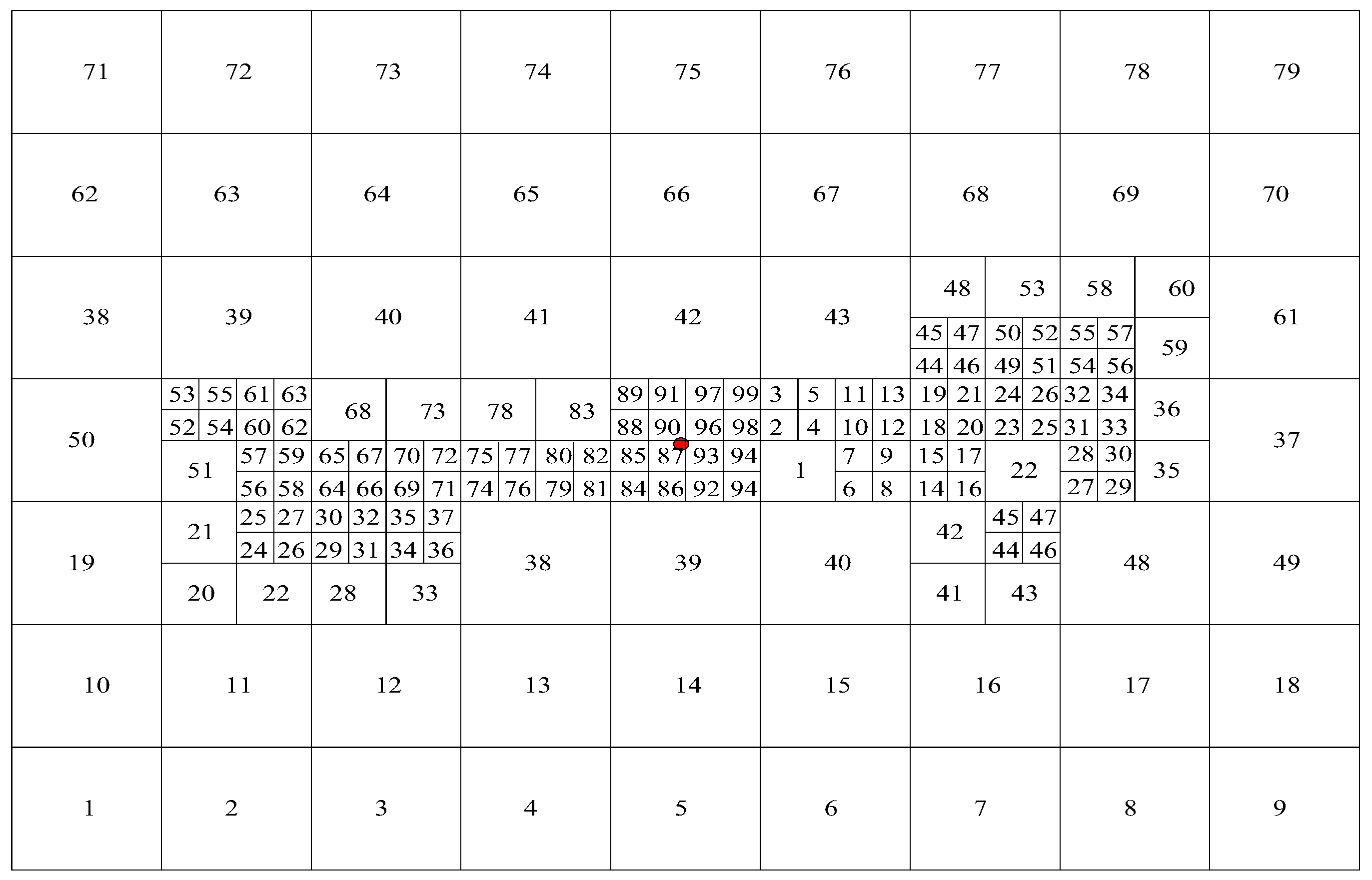
• Local grid refinement

Seen from Figure 3, the entire grid system will be divided into several layers. In this paper, there is a two-fold difference of space step between the adjacent layers. The grid refinement process is to interpolate the coarse-grid variable on the covered finest grids, and then calculate the variables for each finest grid. The linear interpolation method is introduced for the grid refinement in this paper, as shown in Figure 6. Grid 1 is taken out and evenly divided into four grid blocks which are, respectively, labeled as southwest block, southeast block, northwest block, and northeast block.

The steps of linear interpolation in the northeast block of grid 1 are as follows:

(1) The adjacent two grids (grid 2 and grid 3) are given. Therefore, the center point of grid 1, grid 2, and grid 3 can determine a plane.

With the variable of T, the linear polynomial on the two-dimensional plane is:

T(x,y) = ax + by + c

(7)

The three grids here are all coarse grids, so the value of T is known. The central coordinates (x_i,y_i) of grid 1, grid 2, and grid 3, and the value T_i corresponding to the three points are respectively substituted into the Equation (7), so the values of a, b and c can be obtained. Then using Equation (7), the coordinate values of each fine grid in the northeast block of grid 1 are respectively substituted, and the interpolation in these fine grids is calculated. With the above method, local grid refinement can be carried out according to the location network fractures.

• Handling of coarse and fine grid contact surfaces

It can be seen from the establishment of the above differential equations that the information of the four surrounding grids needs to be used. However, using local grid refinement, the center points of fine grid and coarse grid are not on the same horizontal line. Here we still use linear interpolation to calculate the pressure of the corresponding position.

As shown in Figure 7, assuming that the right side of grid 1 touches two grids, grid 2 and grid 3, respectively, the size of grid 2 and grid 3 is the same according to the grid refinement method.

In order to deal with the contact mode of Figure 7, it is assumed that the two sides of the contact interface are flow-conserved, and the pressure inside the same grid has a linear distribution. It is assumed that grid 1 is the k layer grid, while the two adjacent grids on the right are in the k + 1 layer grid. Seen from Figure 7, the contact interface is represented by a and b, respectively, and the auxiliary pressures p₄ and p₅ are, respectively, introduced at the midpoints of the interfaces a and b.

So, point 1, point 4 and point 5 can form a plane, then the expression of the pressure on the plane can be obtained according to the polynomial relationship, namely:

p(x,y) = f(p₁,p₄,p₅,x₁,x₄,x₅,y₁,y₄,y₅)

where, p₁ is known, p₄ and p₅ are unknown. The linear polynomial is assumed to be:

p(x,y) = ax + by + c

(8)

That is,

p₁ = ax₁ + by₁ + c

p₄ = ax₄ + by₄ + c

p₅ = ax₅ + by₅ + c

The linear equations are solved to obtain the unknown quantities a, b, and c. Meanwhile, the auxiliary point 6 and point 7 are given, and the two auxiliary points are symmetrically with points 2 and 3 related to the contact interface. The coordinates of point 6 and point 7 are introduced into Equation (10) to obtained p₆ and p₇. Since p₄ and p₅ are unknown, then p₆ and p₇ are functions of p₄ and p₅.

From the equal flow on both sides of the contact interface, we can get:

$$\left(\frac{k_{1x}}{\mu B}\right)\frac{(p_4-p_6)}{(x_4-x_6)}=\left(\frac{k_{2x}}{\mu B}\right)\frac{(p_2-p_4)}{(x_2-x_4)}$$

(9)

$$\left(\frac{k_{1x}}{\mu B}\right)\frac{(p_5-p_7)}{(x_5-x_7)}=\left(\frac{k_{3x}}{\mu B}\right)\frac{(p_3-p_5)}{(x_3-x_5)}$$

(10)

Therefore, the pressure p₄ and p₅ on the interface a and b can be obtained by using Equations (9) and (10). Then the total flow through the contact interface can be expressed as:

$$T_{xi+1/2}(p_{i+1,j}^{n+1}-p_{i,j}^{n+1})=\left(\frac{k_{1}h\Delta y_j}{B\mu }\right)\frac{(p_5-p_7)+(p_4-p_6)}{\Delta x_i/2}$$

(11)

If the current grid is grid 2, then:

$$T_{xi-1/2}(p_{i,j}^{n+1}-p_{i-1,j}^{n+1})=\left(\frac{k_{1}h\Delta y_j}{B\mu }\right)\frac{(p_2-p_4)}{\Delta x_i}$$

(12)

The total flow here is expressed in the form of $T_{xi+1/2}(p_{i+1,j}^{n+1}-p_{i,j}^{n+1})$ and $T_{xi-1/2}(p_{i,j}^{n+1}-p_{i-1,j}^{n+1})$, and i and j represent the number of the current operational grid in the grid system.

• Numeral order

In the grid refinement, the contact relationship between the grids has the characteristics of variability, so the coefficient matrix structure produced by the different sorting of these grids is different. Therefore, the selection of appropriate grid sorting is also very important. Figure 8 shows the grid numbering method after grid refinement. In the sorting method, the grid layers are ignored and the different layer grids are numbered sequentially. The advantage of this sorting method is that it will not generate invalid numbers and is easier to solve.

3.3. Treatment of Boundary Conditions

The outer boundary of the reservoir is closed and bottom hole pressure is fixed. So, the inner boundary can be expressed as:

$$Q_{vi,j}=PI(p_{i,j}-p_{wf})$$

(13)

The outer boundary can be expressed as:

$$\begin{array}{c}{\frac{\partial p}{\partial x}|}_{i=1/2}=0\\ {\frac{\partial p}{\partial y}|}_{j=1/2}=0\\ {\frac{\partial p}{\partial x}|}_{i=N_x+1/2}=0\\ {\frac{\partial p}{\partial y}|}_{j=N_y+1/2}=0\end{array}\}$$

(14)

A circle of virtual grid is created outside the closed boundary, and the pressure of the virtual grid is equal to the pressure of outer boundary.

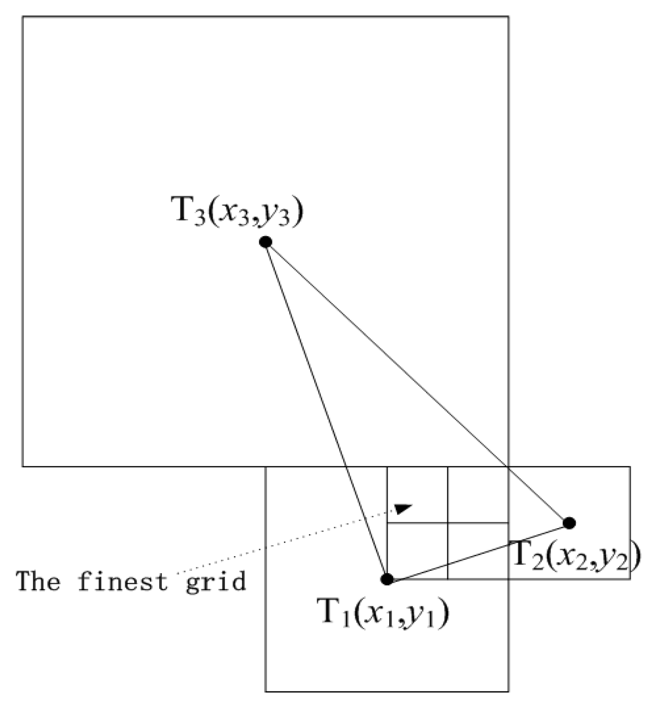
3.4. Treatment of Fracture System

After grid refinement, the parameters of the grid where the fracture is located should be assigned.

Suppose the position of the center point of the grid is (x₀, y₀), the grid width in the x direction is w_x, the grid width in the y direction is w_y, the grid permeability of the corresponding fracture is k_f, the width of the fracture is w_f, and the angle between the fracture and the grid is $\alpha$.

Then the permeability of the grid in the x direction and y direction can be expressed as:

$$k_x(x_0,y_0)=\frac{{\beta }_1{k}_f{w}_f\cos (\alpha )}{w_x}$$

(15)

$$k_y(x_0,y_0)=\frac{{\beta }_2{k}_f{w}_f\sin (\alpha )}{w_y}$$

(16)

3.5. Treatment of Transmission Coefficient

In the above difference equation, the value of $T_{xi\pm 1/2}$ and $T_{yi\pm 1/2}$ is needed. In this paper, the two values are calculated by means of harmonic average, namely:

$$T_{xi\pm 1/2}=\frac{2T_{xi}\cdot T_{xi\pm 1}}{T_{xi}+T_{xi\pm 1}}$$

(17)

where, $T_{xi}={\left(\frac{k}{B\mu }\right)}_i\frac{\Delta y_j\cdot h}{\Delta x_i}$, $T_{xi-1}={\left(\frac{k}{B\mu }\right)}_{i-1}\frac{\Delta y_j\cdot h}{\Delta x_{i-1}}$, $T_{xi+1}={\left(\frac{k}{B\mu }\right)}_{i+1}\frac{\Delta y_j\cdot h}{\Delta x_{i+1}}$.

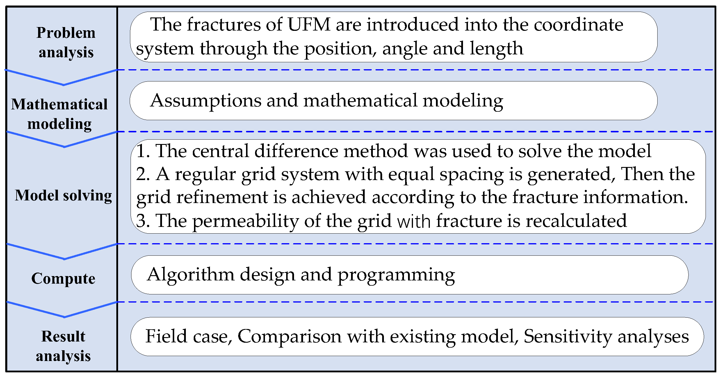
3.6. Calculation Steps and Procedures

With the above model and numerical calculation methods, the numerical simulation of production rate based on the UFM can be performed.

The workflow is shown in Figure 9. The steps are as follows:

(1) Input parameters of the model.

(2) A regular grid system with equal spacing is generated and each grid is assigned the reservoir parameters. Then the grid refinement is achieved according to the fracture information.

(3) The permeability of the grid with fracture is calculated according to Equations (15) and (16).

(4) Set t = 1;

(5) According to the information of the grid system and the pressure distribution at the previous time (when t = 1, the pressure of the previous time is the original formation pressure p_i), the coefficient matrix A and the linear equation group AP = B are obtained. Solve the AP = B, and then set t = t + 1.

(6) Whether the equation of t < t_max is correct. If yes, go to step (7). If no, return to step (5).

(7) Output simulation results, including reservoir pressure distribution and production rate.

(8) End.

4. Field Case and Sensitivity Analyses

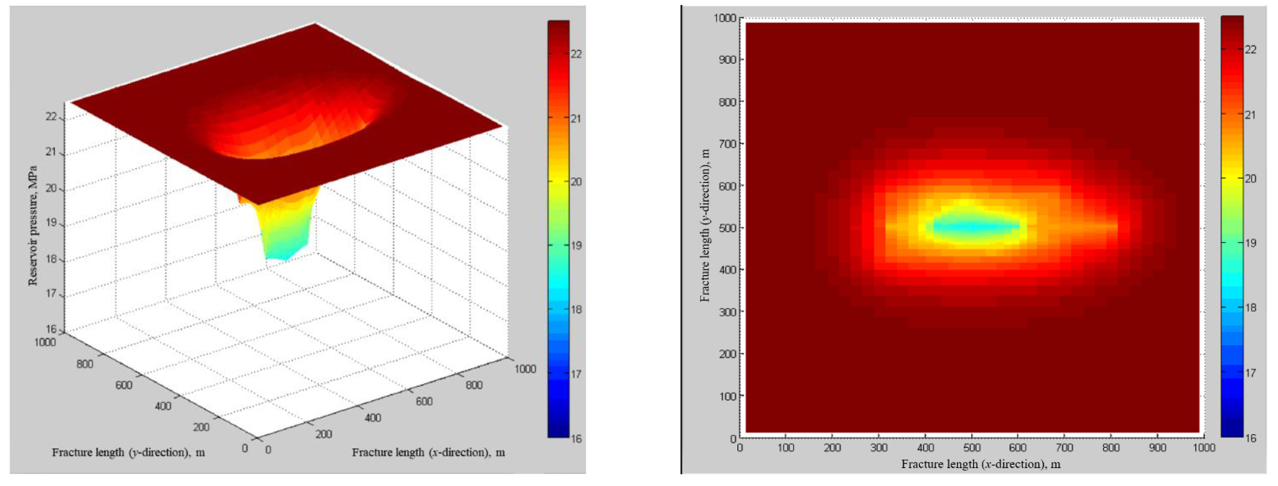
4.1. Field Application

To prove applicability of new method for field cases, a history match is performed.

To the development of natural fractures in the reservoir, the UFM [30] is used to simulate the fracture network system. The simulated results are shown in Figure 10, and the simulated fracture conductivity is 23.5 D·cm. The parameters of the model are presented in

Table 2. Reservoir parameters of well A.

Parameter	Value	Parameter	Value
Reservoir permeability, mD	0.55	Porosity, %	9.2
Initial pressure, MPa	22.5	Reservoir thickness, m	15.5

.

The well is produced with 16 MPa of bottom hole pressure. According to the network fracture simulation results, the detailed information of each fracture is extracted and each fracture is numbered. Then, the information of fracture network is input into the model for prediction of production rate.

The history matching parameters are ${\beta }_1$ and in Equations (15) and (16). In this paper, the initial ${\beta }_1$ and ${\beta }_2$ are 1.00. The parameters values are gradually adjusted for history match. The final value of ${\beta }_1$ is 0.78 and the final value of ${\beta }_2$ is 0.81. The final results are shown in Figure 11. The model can achieve good matching results.

The simulation results are shown in Figure 12, Figure 13 and Figure 14, which are three-dimensional and two-dimensional graphs of pressure distribution for 100 days, 1 year and 2 years respectively. In Figure 12, Figure 13 and Figure 14, the main fracture of the fracture system is placed on the x-axis. So, the fracture system in the upper part of Figure 10 is placed on the right side in the pressure distribution graph, and the fracture system in the lower part of Figure 10 is placed on the left side in the pressure distribution graph. It can be seen from Figure 10 that the fracture system is asymmetrical, and the density of the fracture system above is significantly higher than that of the fracture system below.

The simulation results in Figure 12, Figure 13 and Figure 14 shows that the pressure drop expansion on the right side is obviously larger than that on the left side, and pressure distribution of the reservoir is the same as expected.

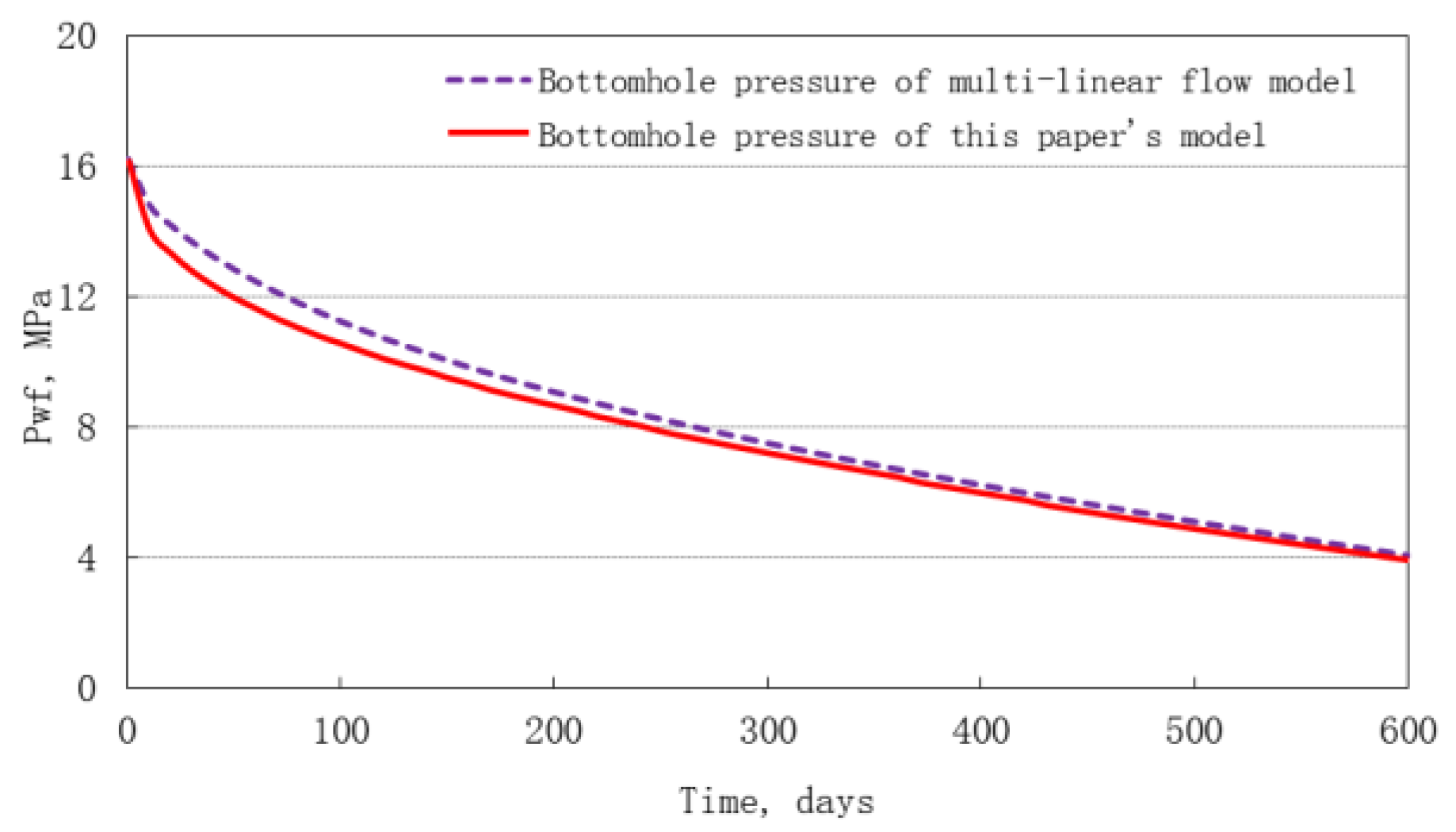
4.2. Comparison with Existing Method

The presented new model is compared with multi-linear flow model [6]. According to the characteristics of fracture networks in the multi-linear flow model, a regular fracture network is adopted for comparison, as shown in Figure 15. The parameters are presented in

Table 3. Model parameters.

Parameter	Value	Parameter	Value
Initial pressure	16.2 MPa	Production rate	20 m3/d
Permeability	0.1 mD	Porosity	0.09
Reservoir length	1000 m	Reservoir width	600 m
Reservoir thickness	15 m	Fracture conductivity	15 D·cm
Fracture spacing	26 m

.

We compared the results of this paper’s model with the results of multi-linear flow model (Figure 16). For the selected model configuration, the results showed excellent agreement. The run time of new model is 15 min.

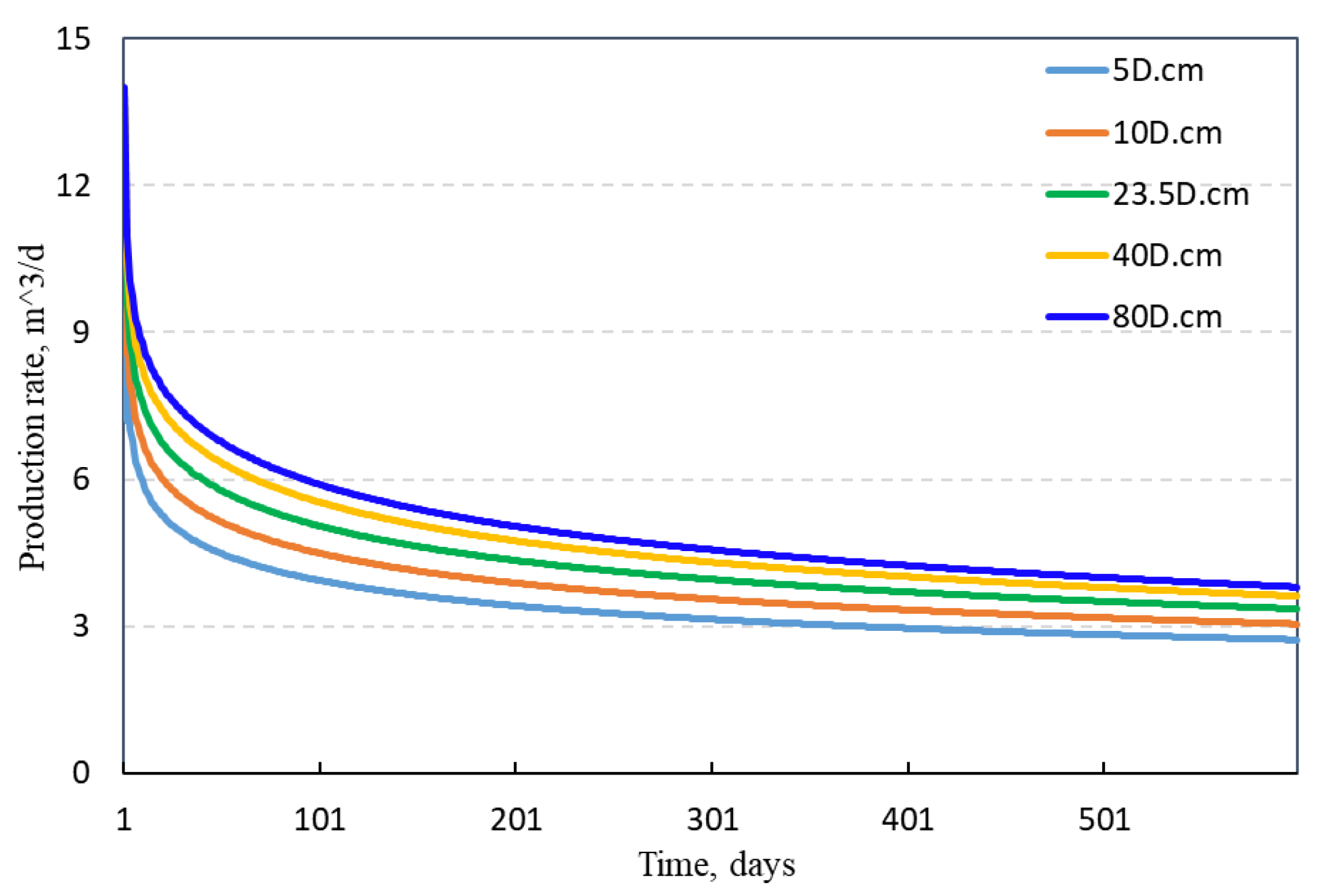
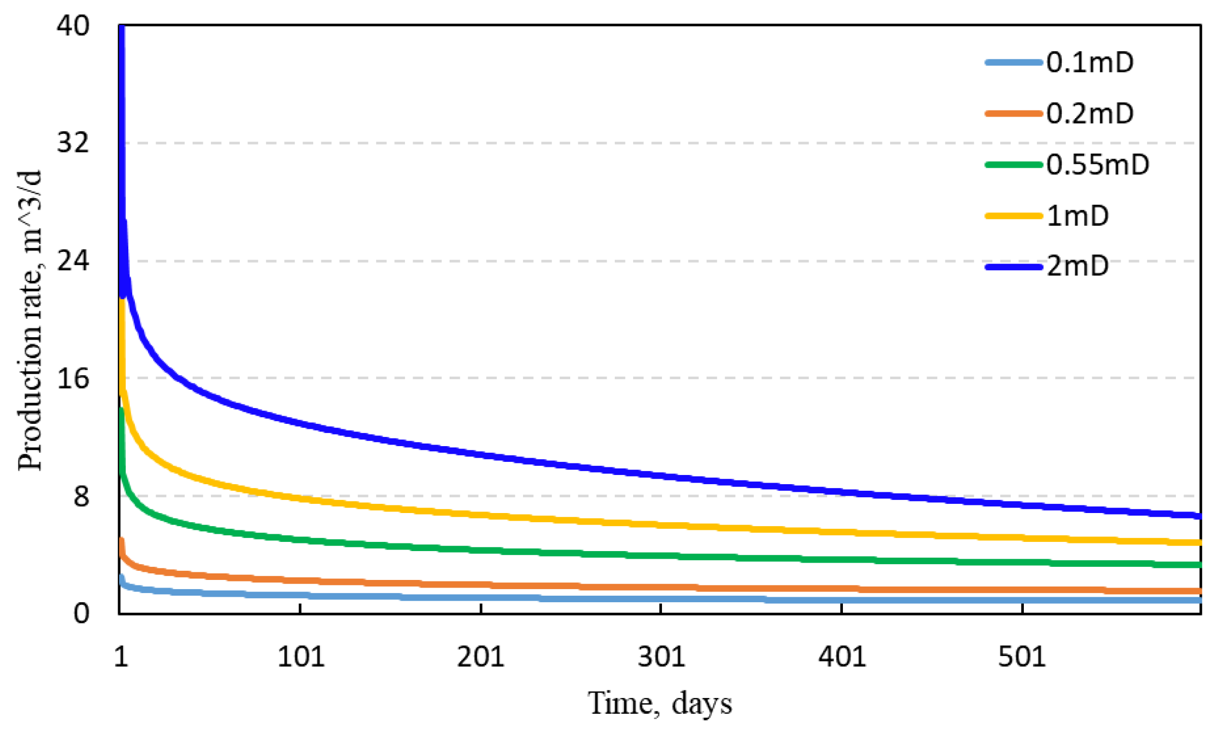
4.3. Sensitivity Analyses

Two properties are discussed by using the new model. The reservoir parameters of Table 2 are used. The parameters discussed include fracture system conductivity and reservoir permeability.

• Fracture system conductivity

Figure 17 shows the impact of the fracture system conductivity on the production rate. We selected five conductivity scenarios of 5 D·cm, 10 D·cm, 23.5 D·cm, 40 D·cm, and 80 D·cm. The conductivity of fracture has a significant influence on production rate. The greater the conductivity, the higher the yield. However, the yield is limited when the conductivity exceeds 40 D·cm.

2.

Reservoir permeability

Figure 18 shows the impact of the reservoir permeability on the production rate. We selected five permeability scenarios of 0.1 mD, 0.2 mD, 0.55 mD, 1 mD, and 2 mD. The permeability has a significant influence on production rate. The greater the permeability, the higher the yield.

4.4. Results and Discussion

Firstly, the new model is applied in field cases to analyze performance in tight oil reservoir with fracture network. According to the fracture parameters of UFM, the detailed information of each fracture in UFM is extracted and numbered. Then, the information of fracture network is input into the model for prediction of production rate. History matching results are shown according to real production data. Compared with the field data, the new model can achieve good matching result. The application of the field case shows that the main advantage of the new model is that it can describe a complex fracture system. Through numerical calculation, the pressure distribution of the reservoir and its change with production time can be given, and the corresponding three-dimensional diagram of pressure distribution can be given. At the same time, the change of production rate with production time can be calculated.

Secondly, the presented new model is compared with multi-linear flow model. When the regular fracture network is adopted, the results of new model showed excellent agreement with existing models. The run time of new model is 15 min. The advantage of this model is that it is more efficient than the conventional numerical method.

Thirdly, according to the characteristics of the new model, the parameters discussed include fracture system conductivity and reservoir permeability. The sensitivity analyses further verified the reliability of the new model.

The disadvantages of the model mainly include the following points. Firstly, the position, angle and length of each fracture in fracture network must be given. Compared with the existing model which simplifies the fracture network, the treatment of the new model is more complex. Secondly, this paper establishes a two-dimensional numerical method, and the description of fracture system is not as precise as the traditional three-dimensional numerical methods. Thirdly, this paper treats fractures as reservoirs with higher permeability in the central difference method, which is simpler and rougher than traditional numerical methods.

5. Conclusions

The purpose of the model in this paper is to present a method for study on the performance analysis of tight reservoir with complex fracture network. The unconventional fracture model (UFM) is one of the commonly used model for the evaluation of fracture system shape and it is necessary to analyze the performance based on detailed fractures information. In this paper, with the numerical simulation method, the analysis model was established. The conclusions are as follows:

(1)

According to the simulation results of the UFM, the fractures are introduced into the coordinate system through the position, angle, and length of the fractures in the fracture system.

(2)

Using unstable seepage model, the reservoir with complex network fracture is treated as heterogeneous reservoir, and then the mathematical model of production rate prediction is established. In the coordinate system, the permeability at the location of fractures is determined by the fracture conductivity.

(3)

According to the characteristics of reservoir and fracture system, local grid refinement method is introduced to describe the network fractures. Based on the mathematical model, the differential equations are first established according to the conventional grid, and then the grid refinement is performed.

(4)

At present, volume fracturing is a popular reservoir stimulation technique, which generates complex fracture systems. The new model can describe complex fracture systems for productivity analysis. According to the fractures shape of UFM, we compared the results between the new model and the field case. The results show acceptable and reasonable matches for typical well. Meanwhile, the presented new model is compared with multi-linear flow model. Finally, the sensitivity of the two properties is discussed. Fracture conductivity and reservoir permeability has a great impact on production rate.

(5)

The presented new model simplifies the analysis of pressure transient and rate transient of reservoir with complex fracture network, and it is more efficient than the conventional numerical method. Compared with the analytical methods, the new model describes the fractures system in more detail. The new model is suitable for production rate modeling of UFM. However, the new model treats fractures as reservoirs with higher permeability in the central difference method, which is simpler and rougher than traditional numerical methods.

References

1. Zhou, W.; Banerjee, R.; Poe, B.D.; Spath, J.; Thambynayagam, M. Semianalytical production simulation of complex hydraulic-fracture networks. SPE J. 2013, 19, 6–18. [Google Scholar] [CrossRef]
2. Ozkan, E.; Brown, M.L.; Raghavan, R.S.; Kazemi, H. Comparison of fractured horizontal-well performance in conventional and unconventional reservoirs. In Proceedings of the SPE Western Regional Meeting, San Jose, CA, USA, 23–26 April 2019. [Google Scholar]
3. Tian, L.; Xiao, C.; Liu, M.; Gu, D.; Song, G.; Cao, H.; Li, X. Well testing model for multi-fractured horizontal well for shale gas reservoirs with consideration of dual diffusion in matrix. J. Nat. Gas Sci. Eng. 2014, 21, 283–295. [Google Scholar] [CrossRef]
4. Stalgorova, E.; Mattar, L. Practical analytical model to simulate production of horizontal wells with branch fractures. In Proceedings of the SPE Canadian Unconventional Resources Conference, Calgary, AB, Canada, 30 October–1 November 2012. [Google Scholar]
5. Al-Rbeawi, S. Analysis of pressure behaviors and flow regimes of naturally and hydraulically fractured unconventional gas reservoirs using multi-linear flow regimes approach. J. Nat. Gas Sci. Eng. 2017, 45, 637–658. [Google Scholar] [CrossRef]
6. Ke, X.; Guo, D.; Zhao, Y.; Zeng, X.; Xue, L. Analytical model to simulate production of tight reservoirs with discrete fracture network using multi-linear flow. J. Pet. Sci. Eng. 2017, 151, 348–361. [Google Scholar] [CrossRef]
7. Zhao, Y.L.; Zhang, L.H.; Luo, J.X.; Zhang, B.N. Performance of fractured horizontal well with stimulated reservoir volume in unconventional gas reservoir. J. Hydrol. 2014, 512, 447–456. [Google Scholar] [CrossRef]
8. Guo, J.; Wang, H.; Zhang, L. Transient pressure and production dynamics of multi-stage fractured horizontal wells in shale gas reservoirs with stimulated reservoir volume. J. Nat. Gas Sci. Eng. 2016, 35, 425–443. [Google Scholar] [CrossRef]
9. Xu, J.; Guo, C.; Teng, W.; Wei, M.; Jiang, R. Production performance analysis of tight oil/gas reservoirs considering stimulated reservoir volume using elliptical flow. J. Nat. Gas Sci. Eng. 2015, 26, 827–839. [Google Scholar] [CrossRef]
10. Zhang, Q.; Su, Y.; Wang, W.; Lu, M.; Ren, L. Performance analysis of fractured wells with elliptical SRV in shale reservoirs. J. Nat. Gas Sci. Eng. 2017, 45, 380–390. [Google Scholar] [CrossRef]
11. Dongyan, F.; Jun, Y.; Hai, S.; Hui, Z.; Wei, W. A composite model of hydraulic fractured horizontal well with stimulated reservoir volume in tight oil & gas reservoir. J. Nat. Gas Sci. Eng. 2015, 24, 115–123. [Google Scholar]
12. Ketineni, S.P.; Ertekin, T. Analysis of production decline characteristics of a multistage hydraulically fractured horizontal well in a naturally fractured reservoir. In Proceedings of the SPE Eastern Regional Meeting, Lexington, KY, USA, 3–5 October 2012. [Google Scholar]
13. Li, Z.; Wu, X.; Han, G.; Zhang, L.; Zhao, R.; Shi, S. A semi-analytical pressure model of horizontal well with complex networks in heterogeneous reservoirs. J. Pet. Sci. Eng. 2021, 202, 108511. [Google Scholar] [CrossRef]
14. Papi, A.; Mohebbi, A.; Eshraghi, S.E. Numerical Simulation of the Impact of Natural Fracture on Fluid Composition Variation Through a Porous Medium. J. Energy Resour. Technol. 2019, 141, 042901. [Google Scholar] [CrossRef]
15. Mayerhofer, M.J.; Lolon, E.P.; Youngblood, J.E.; Heinze, J.R. Integration of microseismic-fracture-mapping results with numerical fracture network production modeling in the Barnett Shale. In Proceedings of the SPE Annual Technical Conference and Exhibition, San Antonio, TX, USA, 24–27 September 2006. [Google Scholar]
16. Cipolla, C.L.; Lolon, E.P.; Erdle, J.C.; Rubin, B. Reservoir modeling in shale-gas reservoirs. SPE Reserv. Eval. Eng. 2010, 13, 638–653. [Google Scholar] [CrossRef]
17. Jia, X.; Filippov, A.; Khoriakov, V.; McNealy, T. An Effective Numerical Model for Fracture-Stimulated Condensate Reservoir Production History Matching, Surveillance, and Prediction. In Proceedings of the Unconventional Resources Technology Conference (URTEC), San Antonio, TX, USA, 1–3 August 2016. [Google Scholar]
18. Xu, W.; Thiercelin, M.J.; Ganguly, U.; Weng, X.; Gu, H.; Onda, H.; Le Calvez, J. Wiremesh: A novel shale fracturing simulator. In Proceedings of the International Oil and Gas Conference and Exhibition in China, Beijing, China, 8–10 June 2010. [Google Scholar]
19. Cipolla, C.L.; Lolon, E.; Mayerhofer, M.J. Reservoir modeling and production evaluation in shale-gas reservoirs. In Proceedings of the International Petroleum Technology Conference, Doha, Qatar, 7–9 December 2009. [Google Scholar]
20. Meyer, B.R.; Bazan, L.W. A discrete fracture network model for hydraulically induced fractures-theory, parametric and case studies. In Proceedings of the SPE Hydraulic Fracturing Technology Conference, The Woodlands, TX, USA, 24–26 January 2011. [Google Scholar]
21. Xiao, C.; Tian, L. Modelling of fractured horizontal wells with complex fracture network in natural gas hydrate reservoirs. Int. J. Hydrogen Energy 2020, 45, 14266–14280. [Google Scholar] [CrossRef]
22. Liu, H.; Zhao, X.; Tang, X.; Peng, B.; Zou, J.; Zhang, X. A Discrete fracture–matrix model for pressure transient analysis in multistage fractured horizontal wells with discretely distributed natural fractures. J. Pet. Sci. Eng. 2020, 192, 107275. [Google Scholar] [CrossRef]
23. Parvizi, H.; Rezaei-Gomari, S.; Nabhani, F. Robust and flexible hydrocarbon production forecasting considering heterogeneity impact for hydraulically fractured wells. Energy Fuels 2017, 31, 8481–8488. [Google Scholar] [CrossRef] [Green Version]
24. Parvizi, H.; Rezaei-Gomari, S.; Nabhani, F.; Turner, A.; Uk, E. Hydraulic Fracturing Performance Evaluation in Tight Sand Gas Reservoirs with High Perm Streaks and Natural Fractures. In Proceedings of the Europec 2015, Madrid, Spain, 1–4 June 2015. SPE-174338-MS. [Google Scholar]
25. Parvizi, H.; Rezaei-Gomari, S.; Nabhani, F.; Dastkhan, Z.; Wei, C.F. A Practical Workflow for Offshore Hydraulic Fracturing Modelling: Focusing on Southern North Sea. In Proceedings of the Europec 2015, Madrid, Spain, 1–4 June 2015; OnePetro: Madrid, Spain, 2015. [Google Scholar]
26. Fisher, M.K.; Heinze, J.R.; Harris, C.D.; Davidson, B.M.; Wright, C.A.; Dunn, K.P. Optimizing horizontal completion techniques in the Barnett shale using microseismic fracture mapping. In Proceedings of the SPE Annual Technical Conference and Exhibition, Houston, TX, USA, 26–29 September 2004. [Google Scholar]
27. Ewing, R.E. Adaptive local grid refinement. In Mathematical and Computational Methods in Seismic Exploration and Reservoir Modeling; Siam: Philadelphia, PA, USA, 1986; Volume 23, p. 235. [Google Scholar]
28. Heinemann, Z.E.; Gerken, G.; von Hantelmann, G. Using local grid refinement in a multiple-application reservoir simulator. In Proceedings of the SPE Reservoir Simulation Symposium, San Francisco, CA, USA, 15–18 November 1983. [Google Scholar]
29. Ke, X.; Guo, D.; Xue, L.; Li, X.; Zhao, Y. Study on Productivity Prediction of Hydraulic Fracturing with Branch Fractures Based on Numerical Simulation Method. Math. Pract. Theory 2019, 49, 89–98. [Google Scholar]
30. Xu, L. The Study on the Menchansim of Fracture Propagation and Numerical Simulation in Volume Fracturing. Doctoral Dissertation, Southwest Petroleum University, Chengdu, China, 2015. [Google Scholar]
Figure 1. The flowchart with detailed procedure of the new method.
Energies 15 04050 g001
Figure 2. The shape of network fracture [26].
Energies 15 04050 g002
Figure 3. Fine description of fracture system (schematic diagram).
Energies 15 04050 g003
Figure 4. Grid system with the local grid refinement.
Energies 15 04050 g004
Figure 5. The corresponding positional relationship between the coefficients and the grids.
Energies 15 04050 g005
Figure 6. Linear interpolation in northeast block of grid 1.
Energies 15 04050 g006
Figure 7. Linear interpolation of pressure and flow conservation at interface.
Energies 15 04050 g007
Figure 8. Grid sorting in local grid refinement. (The red dot refers to the wellbore).
Energies 15 04050 g008
Figure 9. The workflow of the computational procedure.
Energies 15 04050 g009
Figure 10. The simulation results of UFM. (The red dot refers to the wellbore and the red lines refer to the fractures).
Energies 15 04050 g010
Figure 11. History matching of production rate.
Energies 15 04050 g011
Figure 12. Reservoir pressure distribution at the time of 100 days.
Energies 15 04050 g012
Figure 13. Reservoir pressure distribution at the time of one year.
Energies 15 04050 g013
Figure 14. Reservoir pressure distribution at the time of two years.
Energies 15 04050 g014
Figure 15. The regular fracture network.
Energies 15 04050 g015
Figure 16. Comparison of this paper’s results with multi-linear flow model results.
Energies 15 04050 g016
Figure 17. Production curves of conductivity effect.
Energies 15 04050 g017
Figure 18. Production curves of permeability effect.
Energies 15 04050 g018