
Reduction of Computational Burden and Accuracy Maximization in Short-Term Load Forecasting


Abstract
:1. Introduction
1.1. Main Problem
1.2. Solution Approach
1.3. Literature Review
1.4. Paper Contributions
1.5. Sections Summary
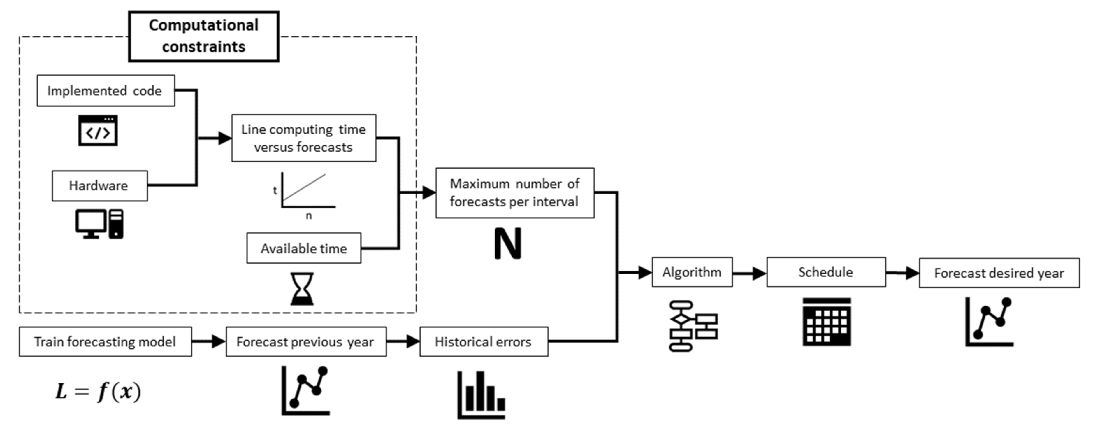
2. Forecasting System Employed
2.1. Forecasting Schedule
2.2. Data Employed
- The training group is employed to train the STLF models, these are the data from the years from 2012 to 2018 inclusive. Therefore, the 7 years prior to the desired year to forecast was selected, as recommended in the analysis of the STLF system performance [18].
- The validation group is used by the algorithm to obtain error records, comprising the year prior to the test period: 2018, therefore it coincides with the last year of training. The validation period coincides with the end of training because it must be done with data from the 7 years prior to the year to be predicted. Moreover, the post-training data cannot be used, since the validation is simulated without it.
- The test group is used to verify the performance of the forecasting system with the implemented algorithm. In this case the year 2019 was selected.
3. Methodology
4. Proposed Algorithm
5. Results
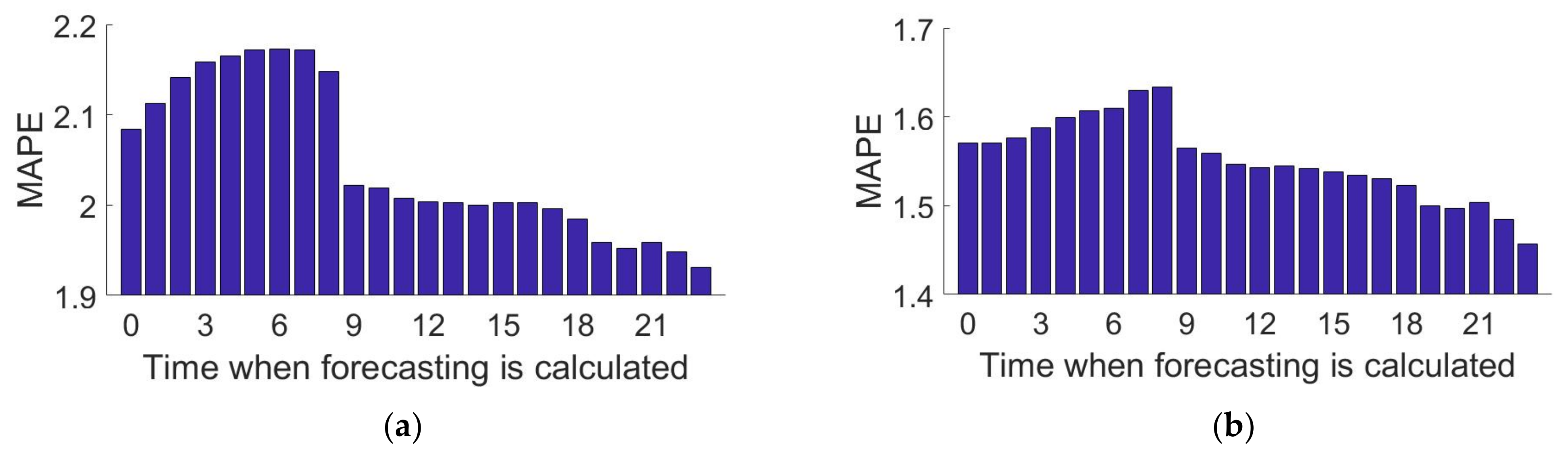
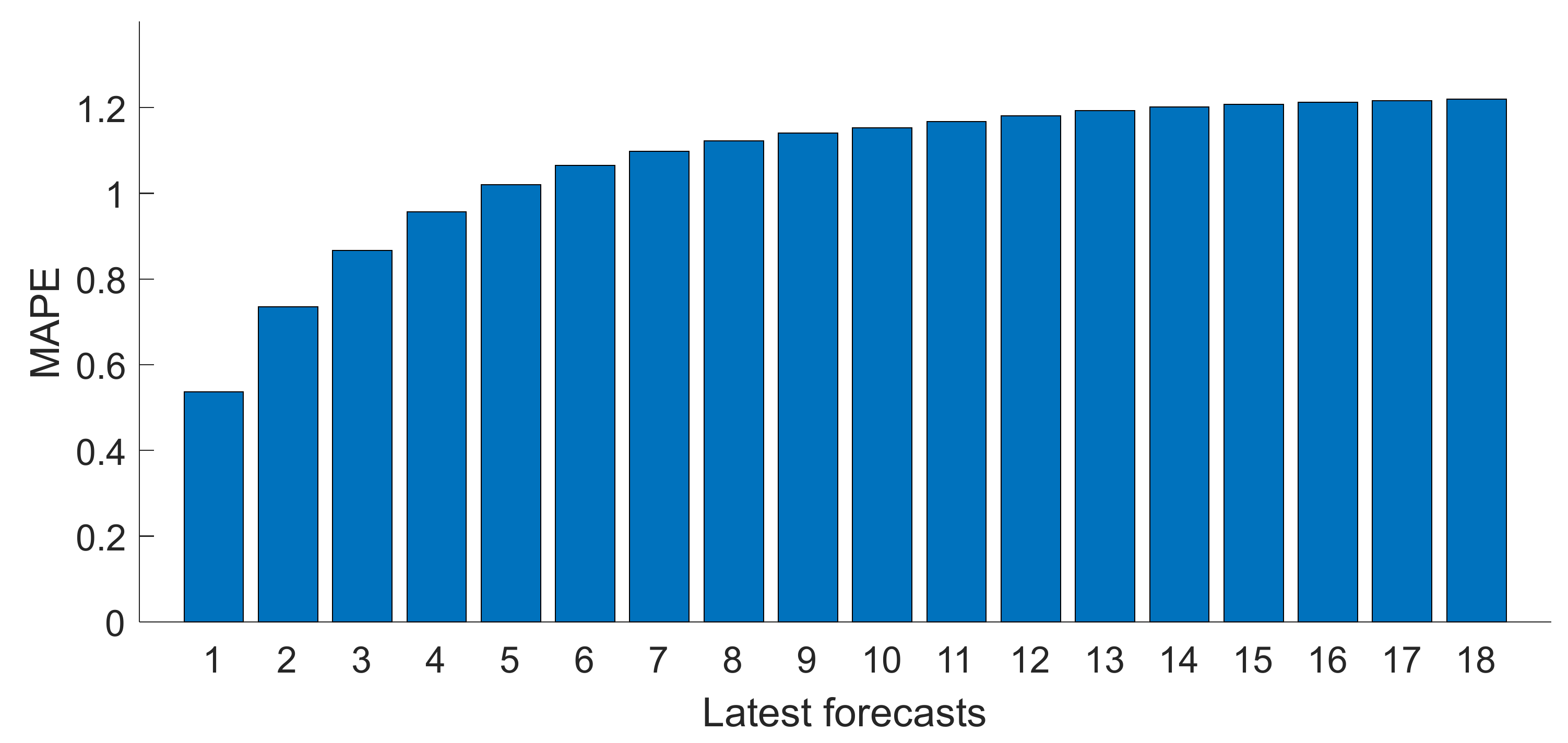
- 1.
- At 9:00 a.m., only 18.3% of forecasts are for the first 8 h of each future day. This allows us to infer that there is usually not a significant accuracy improvement in forecasting the first 8 h of each future day at 9:00 a.m. This conclusion is further developed in Section 5.1. “Temperature Influence on Early Morning”.
- 2.
- At 9:00 a.m., only 5.6% of the predictions executed correspond to the first 4 days (including the current day). This selection makes sense since obtaining temperature data benefits more distant days than close ones, as seen in Section 5.1 “Temperature Influence on distant days”.
- 3.
- For all running hours, the next hour is always forecast; while 22 of 24 running hours forecast the next two future hours and 21 of 24 forecast the next three. This fact coincides with the reasoning from Section 5.1 “Recent Loads”, as it states that hours prior to the forecast moment tend to perform a great accuracy improvement.
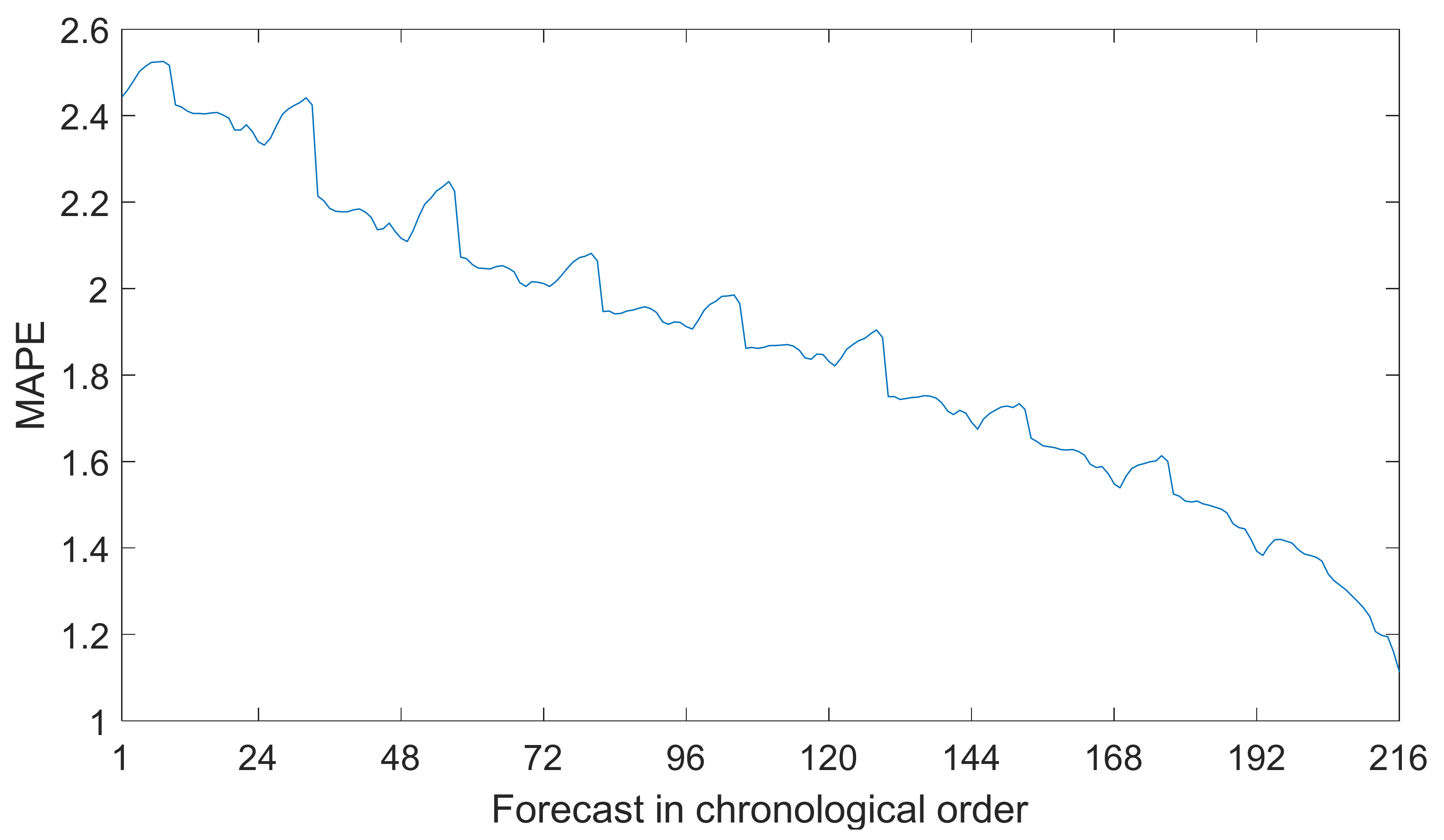
5.1. Error Analysis
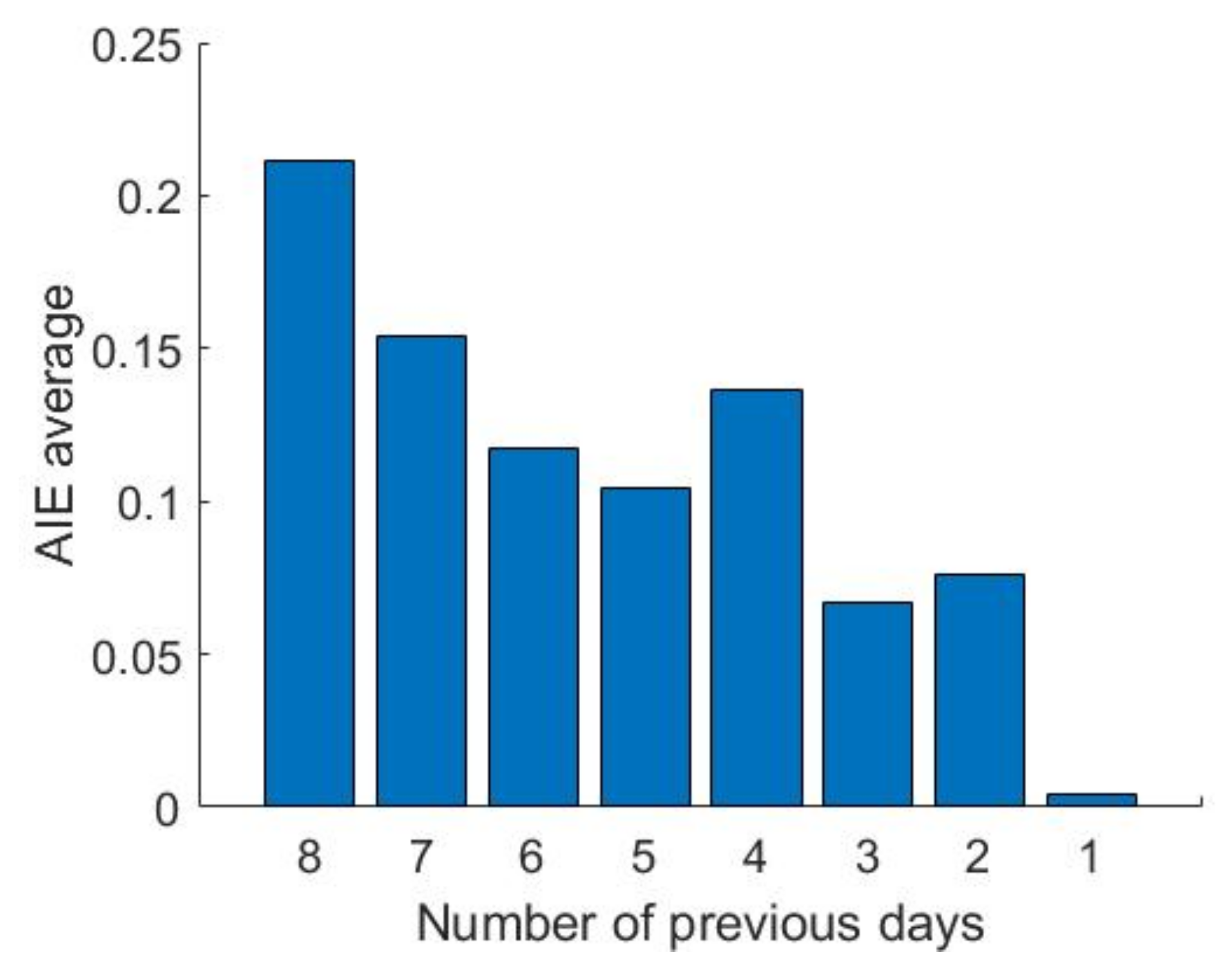
5.1.1. AIE and Error Analysis
Temperature Influence on Early Morning
Temperature Influence on Distant Days
Recent Loads
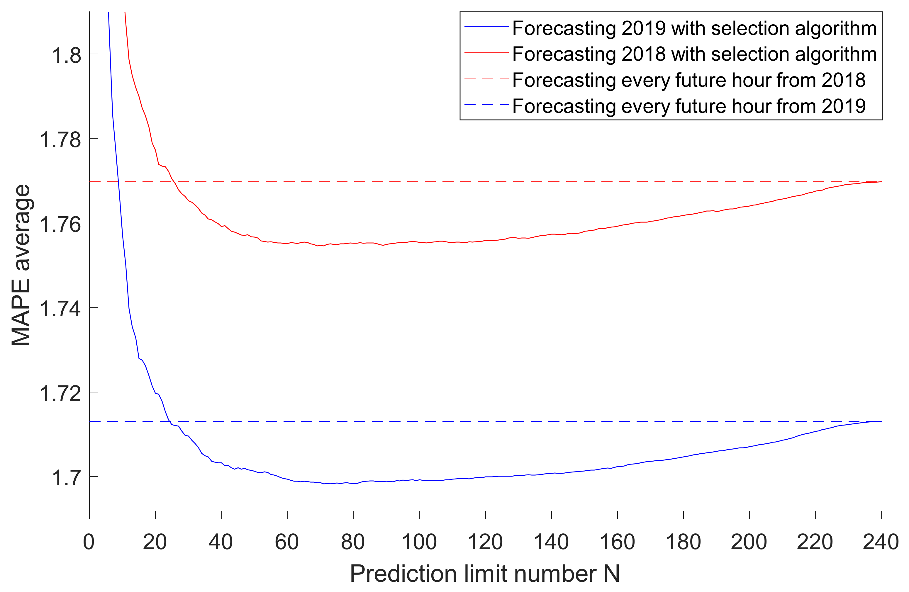
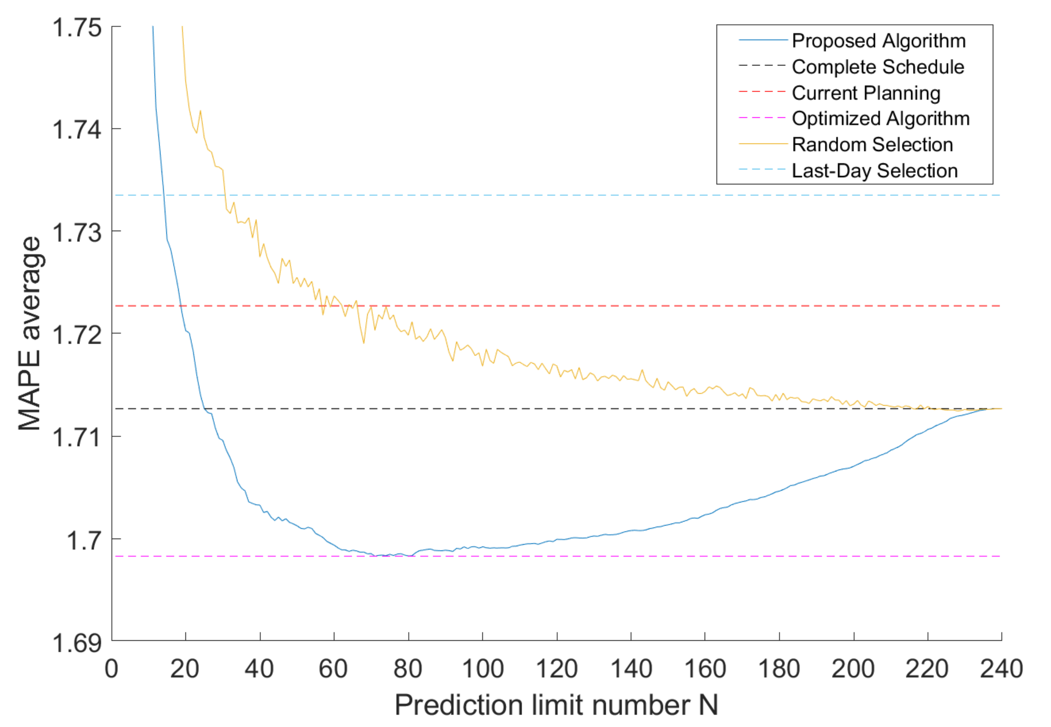
5.2. Obtaining the Optimal Forecast Number
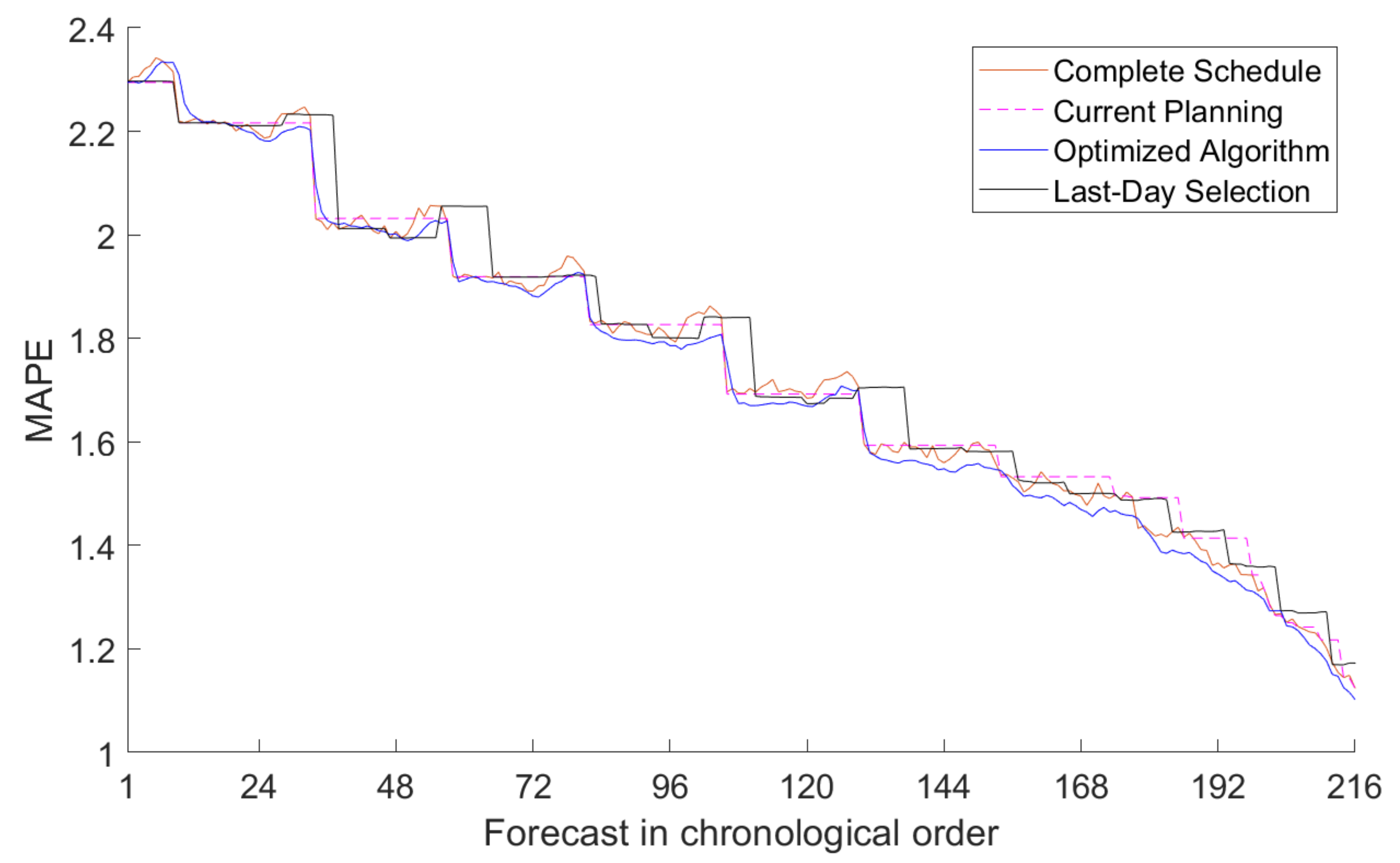
5.3. Accuracy Results of Optimized Scheduling
5.4. Computational Burden
6. Conclusions
Author Contributions
Funding
Institutional Review Board Statement
Informed Consent Statement
Data Availability Statement
Acknowledgments
Conflicts of Interest
References
- Zhang, Z.; Dou, C.; Yue, D.; Zhang, B. Predictive Voltage Hierarchical Controller Design for Islanded Microgrids Under Limited Communication. IEEE Trans. Circuits Syst. Regul. Pap. 2022, 69, 933–945. [Google Scholar] [CrossRef]
- Han, L.; Peng, Y.; Li, Y.; Yong, B.; Zhou, Q.; Shu, L. Enhanced Deep Networks for Short-Term and Medium-Term Load Forecasting. IEEE Access 2019, 7, 4045–4055. [Google Scholar] [CrossRef]
- Hong, T.; Wilson, J.; Xie, J. Long Term Probabilistic Load Forecasting and Normalization With Hourly Information. IEEE Trans. Smart Grid 2014, 5, 456–462. [Google Scholar] [CrossRef]
- Kong, W.; Dong, Z.Y.; Hill, D.J.; Luo, F.; Xu, Y. Short-Term Residential Load Forecasting Based on Resident Behaviour Learning. IEEE Trans. Power Syst. 2018, 33, 1087–1088. [Google Scholar] [CrossRef]
- Chen, Q.; Xia, M.; Lu, T.; Jiang, X.; Liu, W.; Sun, Q. Short-Term Load Forecasting Based on Deep Learning for End-User Transformer Subject to Volatile Electric Heating Loads. IEEE Access 2019, 7, 162697–162707. [Google Scholar] [CrossRef]
- Niu, D.-X.; Wanq, Q.; Li, J.-C. Short term load forecasting model using support vector machine based on artificial neural network. In Proceedings of the 2005 International Conference on Machine Learning and Cybernetics, Guangzhou, China, 18–21 August 2005; Volume 7, pp. 4260–4265. [Google Scholar]
- Singh, S.; Hussain, S.; Bazaz, M.A. Short Term Load Forecasting Using Artificial Neural Network. In Proceedings of the 2017 Fourth International Conference on Image Information Processing (ICIIP), Shimla, India, 21–23 December 2017; p. 5. [Google Scholar]
- Chen, K.; Chen, K.; Wang, Q.; He, Z.; Hu, J.; He, J. Short-Term Load Forecasting With Deep Residual Networks. IEEE Trans. Smart Grid 2019, 10, 3943–3952. [Google Scholar] [CrossRef] [Green Version]
- Wang, P.; Liu, B.; Hong, T. Electric load forecasting with recency effect: A big data approach. Int. J. Forecast. 2016, 32, 585–597. [Google Scholar] [CrossRef] [Green Version]
- Yang, L.; Yang, H. A Combined ARIMA-PPR Model for Short-Term Load Forecasting. In Proceedings of the 2019 IEEE Innovative Smart Grid Technologies—Asia (ISGT Asia), Chengdu, China, 21–24 May 2019; pp. 3363–3367. [Google Scholar]
- López, M.; Valero, S.; Rodriguez, A.; Veiras, I.; Senabre, C. New online load forecasting system for the Spanish Transport System Operator. Electr. Power Syst. Res. 2018, 154, 401–412. [Google Scholar] [CrossRef]
- Bianchi, F.M.; De Santis, E.; Rizzi, A.; Sadeghian, A. Short-Term Electric Load Forecasting Using Echo State Networks and PCA Decomposition. IEEE Access 2015, 3, 1931–1943. [Google Scholar] [CrossRef]
- Ma, Y.; Zhang, Q.; Ding, J.; Wang, Q.; Ma, J. Short Term Load Forecasting Based on iForest-LSTM. In Proceedings of the 2019 14th IEEE Conference on Industrial Electronics and Applications (ICIEA), Xi’an, China, 19–21 June 2019; pp. 2278–2282. [Google Scholar]
- Abedinia, O.; Amjady, N.; Zareipour, H. A New Feature Selection Technique for Load and Price Forecast of Electrical Power Systems. IEEE Trans. Power Syst. 2017, 32, 62–74. [Google Scholar] [CrossRef]
- Mamun, A.A.; Sohel, M.; Mohammad, N.; Haque Sunny, M.S.; Dipta, D.R.; Hossain, E. A Comprehensive Review of the Load Forecasting Techniques Using Single and Hybrid Predictive Models. IEEE Access 2020, 8, 134911–134939. [Google Scholar] [CrossRef]
- Hippert, H.S.; Pedreira, C.E.; Souza, R.C. Neural networks for short-term load forecasting: A review and evaluation. IEEE Trans. Power Syst. 2001, 16, 44–55. [Google Scholar] [CrossRef]
- Hong, T.; Fan, S. Probabilistic electric load forecasting: A tutorial review. Int. J. Forecast. 2016, 32, 914–938. [Google Scholar] [CrossRef]
- López, M.; Sans, C.; Valero, S.; Senabre, C. Empirical Comparison of Neural Network and Auto-Regressive Models in Short-Term Load Forecasting. Energies 2018, 11, 2080. [Google Scholar] [CrossRef] [Green Version]
- Sethi, R.; Kleissl, J. Comparison of Short-Term Load Forecasting Techniques. In Proceedings of the 2020 IEEE Conference on Technologies for Sustainability (SusTech), Santa Ana, CA, USA, 23–25 April 2020; pp. 1–6. [Google Scholar]
- Jie-sheng, W.; Qing-wen, Z. Short-term electricity load forecast performance comparison based on four neural network models. In Proceedings of the The 27th Chinese Control and Decision Conference (2015 CCDC), Qingdao, China, 23–25 May 2015; pp. 2928–2932. [Google Scholar]
- Mehmood, S.T.; El-Hawary, M. Performance Evaluation of New and Advanced Neural Networks for Short Term Load Forecasting. In Proceedings of the 2014 IEEE Electrical Power and Energy Conference, Calgary, AB, Canada, 12–14 November 2014; pp. 202–207. [Google Scholar]
- Sun, X.; Luh, P.B.; Cheung, K.W.; Guan, W.; Michel, L.D.; Venkata, S.S.; Miller, M.T. An Efficient Approach to Short-Term Load Forecasting at the Distribution Level. IEEE Trans. Power Syst. 2016, 31, 2526–2537. [Google Scholar] [CrossRef]
- Rafi, S.H.; Nahid-Al-Masood, N.-A.-M. Highly Efficient Short Term Load Forecasting Scheme Using Long Short Term Memory Network. In Proceedings of the 2020 8th International Electrical Engineering Congress (iEECON), Chiang Mai, Thailand, 4–6 March 2020; pp. 1–4. [Google Scholar]
- Kong, W.; Dong, Z.Y.; Jia, Y.; Hill, D.J.; Xu, Y.; Zhang, Y. Short-Term Residential Load Forecasting Based on LSTM Recurrent Neural Network. IEEE Trans. Smart Grid 2019, 10, 841–851. [Google Scholar] [CrossRef]
- Rafi, S.H.; Nahid-Al-Masood; Deeba, S.R.; Hossain, E. A Short-Term Load Forecasting Method Using Integrated CNN and LSTM Network. IEEE Access 2021, 9, 32436–32448. [Google Scholar] [CrossRef]
- Mohammed, J.; Bahadoorsingh, S.; Ramsamooj, N.; Sharma, C. Performance of exponential smoothing, a neural network and a hybrid algorithm to the short term load forecasting of batch and continuous loads. In Proceedings of the 2017 IEEE Manchester Power Tech, Manchester, UK, 18–22 June 2017; pp. 1–6. [Google Scholar]
- Veljanovski, G.; Atanasovski, M.; Kostov, M.; Popovski, P. Application of Neural Networks for Short Term Load Forecasting in Power System of North Macedonia. In Proceedings of the 2020 55th International Scientific Conference on Information, Communication and Energy Systems and Technologies (ICEST), Niš, Serbia, 10–12 September 2020; pp. 99–101. [Google Scholar]
- Weyermüller, E.; Vermeulen, H.J.; Groch, M. Short-Term Load Forecasting using Minimalistic Adaptive Neuro Fuzzy Inference Systems. In Proceedings of the 2020 International SAUPEC/RobMech/PRASA Conference, Cape Town, South Africa, 29–31 January 2020; pp. 1–6. [Google Scholar]
- Liu, S.; Gu, S.; Bao, T. An Automatic Forecasting Method for Time Series. Chin. J. Electron. 2017, 26, 445–452. [Google Scholar] [CrossRef]
- Panapongpakorn, T.; Banjerdpongchai, D. Short-Term Load Forecast for Energy Management Systems Using Time Series Analysis and Neural Network Method with Average True Range. In Proceedings of the 2019 First International Symposium on Instrumentation, Control, Artificial Intelligence, and Robotics (ICA-SYMP), Bangkok, Thailand, 16–18 January 2019; pp. 86–89. [Google Scholar]
- Di, S. Power System Short Term Load Forecasting Based on Weather Factors. In Proceedings of the 2020 3rd World Conference on Mechanical Engineering and Intelligent Manufacturing (WCMEIM), Shanghai, China, 4–6 December 2020; pp. 694–698. [Google Scholar]
- Jiang, H.; Zhang, Y.; Muljadi, E.; Zhang, J.J.; Gao, D.W. A Short-Term and High-Resolution Distribution System Load Forecasting Approach Using Support Vector Regression With Hybrid Parameters Optimization. IEEE Trans. Smart Grid 2018, 9, 3341–3350. [Google Scholar] [CrossRef]
- McIlvenna, A.; Herron, A.; Hambrick, J.; Ollis, B.; Ostrowski, J. Reducing the computational burden of a microgrid energy management system. Comput. Ind. Eng. 2020, 143, 106384. [Google Scholar] [CrossRef]
- Weimar, M.; Somani, A.; Etingov, P.; Miller, L.; Makarov, Y.; Loutan, C.; Katzenstein, W. Benefit Cost Analysis of Improved Forecasting for Day-Ahead Hourly Regulation Requirements. In Proceedings of the 2018 IEEE Power Energy Society General Meeting (PESGM), Portland, OR, USA, 5–10 August 2018; pp. 1–5. [Google Scholar]
- López, M.; Sans, C.; Valero, S.; Senabre, C. Classification of Special Days in Short-Term Load Forecasting: The Spanish Case Study. Energies 2019, 12, 1253. [Google Scholar] [CrossRef] [Green Version]


| (a) | (b) | ||||||||||
|---|---|---|---|---|---|---|---|---|---|---|---|
| Run Time | Future Day Whose Load Is Forecast | Run Time | Future Day Whose Load Is Forecast | ||||||||
| Current Day | 1 | 2 | 3–8 | 9 | Current Day | 1 | 2 | 3–8 | 9 | ||
| 0 | 0–23 | 12 | 12–23 | ||||||||
| 1 | 13 | 13–23 | 0–23 | ||||||||
| 2 | 14 | 14–23 | |||||||||
| 3 | 3–23 | 15 | 15–23 | ||||||||
| 4 | 16 | 16–23 | |||||||||
| 5 | 5–23 | 0–23 | 0–23 | 17 | 17–23 | 0–23 | 0–23 | ||||
| 6 | 18 | 18–23 | |||||||||
| 7 | 7–23 | 0–23 | 19 | 19–23 | |||||||
| 8 | 8–23 | 0–23 | 0–23 | 20 | 20–23 | ||||||
| 9 | 9–23 | 0–23 | 0–23 | 0–23 | 21 | 21–23 | 0–23 | ||||
| 10 | 10–23 | 22 | 22–23 | ||||||||
| 11 | 11–23 | 0–23 | 23 | 23 | 0–23 | ||||||
| Name | Explanation |
|---|---|
| Proposed algorithm | Employ the proposed algorithm to obtain a schedule and then use it to forecast during the entire year. |
| Complete schedule | Predict every future intervals up to 9 days in advance, at every hour of the day. |
| Current planning | Use the current schedule from REE, which is explained with Table 1. |
| Optimized algorithm | Employ the proposed algorithm with the optimal forecast number. |
| Random selection | Forecast a number, N, of random future intervals at each hour of the day. |
| Last-day selection | This algorithm, at each moment, predicts the current day. It also forecasts the future day that has gone the longest time without updating, prioritizing those days which have never been forecast. |
| Run Time | Future Day Whose Load Is Forecast | |||||||||
|---|---|---|---|---|---|---|---|---|---|---|
| Current Day | 1 | 2 | 3 | 4 | 5 | 6 | 7 | 8 | 9 | |
| 0 | 0–1, 5, 9, 23 | 0, 18, 22 | 2–5, 10, 14, 16–18, 22–23 | 1, 10, 19, 21–23 | 4, 18, 22 | 2, 4, 13, 16, 22 | 11, 14, 22–23 | 2, 19–20, 23 | 2, 7, 12, 16, 22–23 | 0–23 |
| 1 | 1–5, 7, 22 | 1–2, 5–6, 9, 11, 23 | 0, 2–3, 7–8, 18–19 | 0–1, 4, 10, 17 | 0–4, 15, 18, 21 | 0, 3, 6–7, 11 | 0, 9, 19–20, 23 | 3, 5, 11–12, 15, 21 | 0, 3, 12, 14, 19 | 0–5, 7–8, 10–11, 13–14, 16–17, 19, 22 |
| 2 | 2–6, 8, 10, 13–14, 22 | 0–1, 6–7, 10–11, 17–18 | 2, 7, 10, 19, 21 | 1–2, 10, 12, 15, 18–19, 22 | 2–3, 12–13, 15, 18, 21 | 5, 10, 12–14, 18, 23 | 10, 12, 14 | 0, 4, 7, 11–12, 18, 21 | 0, 3, 12–13 | 0, 5–6, 9–14, 17, 19, 22 |
| 3 | 3–7, 9, 12–13, 18, 20 | 1–4, 6–7, 10, 12, 21 | 0, 6–7, 11, 18–19, 23 | 4, 8, 10, 13–14, 18–20 | 2–3, 13–14, 17–18, 22 | 3, 12, 15, 18 | 0, 2, 13, 19, 22–23 | 0, 11, 13, 23 | 0, 3, 11–14, 23 | 2–4, 9, 13–15, 18, 22 |
| 4 | 4–7, 10, 14, 16, 19, 22 | 1–6, 8, 10, 13, 18–19 | 1, 4, 7, 10, 15, 18–19, 21, 23 | 2–4, 7, 10, 12–13, 19 | 0, 2–3, 5, 17–18, 22 | 3, 10, 13, 15 | 11–12, 14–15, 17, 19, 23 | 0, 10, 12, 16, 18, 22 | 3, 12, 18 | 4, 10–12, 14, 18, 23 |
| 5 | 5–8, 12, 14, 16–17, 20–21 | 2, 4–5, 7, 17, 19 | 2, 5, 7, 10–11, 17, 21 | 7, 12–15, 17–20 | 2–3, 10, 13, 16, 18, 21–22 | 2, 4–5, 10, 12, 16–17, 22–23 | 8, 12, 15, 20, 23 | 0, 10, 12, 15, 18, 23 | 11, 19, 23 | 0, 5, 7, 11–13, 15, 18 |
| 6 | 6–9, 12, 14, 17, 19, 21, 23 | 0, 3–7, 9, 17, 20, 23 | 0, 3, 14–15, 22 | 1–2, 4–5, 9, 12–14, 16–18 | 2–3, 8, 12, 17–18, 21 | 2, 6, 13–14, 16, 22 | 0, 9, 15, 17, 22 | 0, 10–11, 15, 21, 23 | 3, 6, 10–11, 13, 18, 23 | 6, 8, 20, 22 |
| 7 | 7–9, 11–20, 22–23 | 0–3, 5–6, 8–9, 15, 18–20, 23 | 0, 2–5, 9, 11–12 | 1, 5, 7, 13, 18 | 2, 16, 22 | 2, 4, 12–14, 16–17, 19, 22 | 0, 8, 15, 19, 21–22 | 0, 11, 21 | 13, 18, 23 | 0, 5, 9–10, 13, 23 |
| 8 | 8–10, 16–18, 23 | 0–1, 4, 6–8, 10–12, 15, 17, 19–20, 23 | 1, 11, 13, 22–23 | 2, 9, 11, 14, 17, 20, 23 | 0, 2, 19, 21 | 4–5, 8, 17–19, 22 | 0, 10, 15, 18, 20–23 | 0, 7, 9, 15, 17, 19, 22–23 | 13, 18–19 | 2, 4, 6, 13, 15, 17, 21, 23 |
| 9 | 9 | 3, 19 | 15 | 0, 2, 8–14, 18, 20–21 | 8, 10, 12–14, 16, 22 | 8–10, 14–23 | 0, 2–7, 10, 13, 15–23 | 3, 6, 9, 13–19, 21–23 | 2, 13, 20–21 | |
| 10 | 10–12, 18 | 6 | 2, 5, 13, 22–23 | 1, 13, 17, 21–23 | 3, 6, 15–17, 19, 22–23 | 0–1, 3–4, 11, 16–21, 23 | 0, 2, 4–5, 11, 13, 22 | 1, 8–9, 11–12, 14, 16 | 0–2, 5–6, 10–12, 20 | 0, 4–6, 10, 12, 15, 17–19, 22–23 |
| 11 | 11–20, 23 | 4, 7–10, 18, 23 | 1–2, 17–18, 21 | 2, 6, 8, 11–12, 14, 18–20, 22–23 | 1, 5, 9, 16–17 | 0, 2, 5–7, 9, 15, 23 | 3, 6–7, 12–13, 23 | 1, 8–9, 18, 20 | 0, 2, 4, 7–8, 15, 22 | 11, 13, 15–17, 20 |
| 12 | 12–17,19–21, 23 | 0, 4, 6, 9, 11,14, 18, 22 | 4, 7–9, 12, 15,17–18, 20–21 | 0, 4, 7, 9–11,13–16, 19–21 | 4, 7, 14, 16, 23 | 1, 5, 15 | 0–1, 6,11–12, 14–16 | 2–4, 7–8, 14 | 1, 3, 7–8 | 1, 14, 17, 23 |
| 13 | 13–23 | 10, 15, 17, 20 | 0, 5, 10, 12, 14, 16, 20–21 | 0–2, 4–5, 13–14, 16, 18, 20, 23 | 7, 13 | 2–3, 5, 12, 17–18 | 1, 6, 11–12, 17, 22 | 0, 2, 5, 8, 11, 14, 16, 18–20 | 0, 3–4, 10, 18, 22 | 3, 7, 9, 11, 13, 16, 19 |
| 14 | 14–19, 21, 23 | 1, 3, 10–12, 14, 16–17, 22 | 4, 11, 13, 15–16, 18–20, 23 | 3, 5, 7, 9, 12, 18–19, 23 | 5, 8, 13–14, 16–17, 21, 23 | 4, 9, 18 | 0–1, 21–23 | 0, 7, 9–10, 12 13, 15–16, 19, 21 | 1, 5, 20 | 1, 3, 11, 15, 17, 19, 22–23 |
| 15 | 15–23 | 0–1, 4–6, 8, 13, 15–17, 23 | 2, 9, 11–13, 16, 20 | 7, 10–12, 14, 16, 20 | 4, 6, 8–9, 12–13, 15, 19–21 | 13–14, 17–18 | 1, 5, 21–22 | 0–1, 4, 8–9, 12–13, 20, 23 | 1, 4, 9, 16–18, 20 | 5, 16, 18 |
| 16 | 16–22 | 0–3, 10–11, 13, 16, 18–19, 22 | 0, 2, 4, 12–13, 17–18, 23 | 1, 9, 11–12, 17–18, 23 | 1, 17–18, 20 | 2, 12, 22 | 2–3, 12–13, 21–22 | 1, 5, 7, 11–13, 15, 18–21, 23 | 2–3, 18, 20 | 1, 3, 6–7, 11–13, 19, 23 |
| 17 | 17–22 | 0, 2–5, 11–13, 15–19, 21 | 1, 4, 10–11, 14, 17–18, 20, 22 | 0, 5, 9–11, 18 | 4, 9, 11, 14–15, 20–21, 23 | 14, 17 | 5, 21, 23 | 0–2, 7, 9, 12, 19, 21, 23 | 1, 11–12, 18–19, 22–23 | 1, 3, 6, 8, 17, 19, 23 |
| 18 | 18–20, 22–23 | 1–2, 5, 9, 11, 13–15, 17, 19–22 | 2, 4, 12, 15–17, 20, 22 | 3, 10–11, 13, 16–17, 19, 21, 23 | 4, 10, 12–15 | 1, 7, 9, 14, 17, 21–22 | 0, 5–6, 8, 12, 18 | 1, 5, 8–9, 11, 15–16, 22–23 | 1, 5, 11, 19–20 | 7, 12–13 |
| 19 | 19–23 | 0, 2, 9, 12–13, 18–20, 22–23 | 12, 14, 16–21 | 11, 14, 16–19, 21, 23 | 0, 2, 12, 14, 20, 22 | 4–5, 13, 17–18, 20–22 | 1–3, 12, 14, 16, 21–23 | 12, 20, 23 | 0–3, 11, 13, 19, 21 | 3, 10, 15, 17, 19–20 |
| 20 | 20–23 | 0, 2, 5, 10, 14–20, 22–23 | 1, 3, 9–11, 16–18, 23 | 10, 15, 18–20 | 2, 14, 16–17, 19–21 | 1, 3, 9, 20–22 | 11, 14–15, 21, 23 | 1, 4, 6, 14, 19, 23 | 0, 2, 4, 8–9, 18, 20–21 | 1, 3–4, 7, 12, 19, 22–23 |
| 21 | 21–23 | 0–2, 4, 8–9, 11, 14, 17, 20, 22–23 | 3, 14, 16–17, 20 | 1, 4, 11, 16, 18–20 | 1–2, 10, 14, 17, 19–21 | 3, 11, 15, 18–23 | 0, 2–3, 13–14, 17, 23 | 4, 8, 12, 14, 16, 18–19, 23 | 3, 11–12, 18, 22–23 | 3, 7, 9, 19–20, 22 |
| 22 | 22–23 | 0–1, 13, 18–21 | 0, 2–4, 9–10, 17–23 | 0, 4, 10–11, 13, 18, 20, 23 | 1, 5, 10, 13, 15, 17–23 | 3, 9, 21–22 | 2–3, 11, 14, 17–18 | 0, 4, 12, 19–20, 23 | 1, 3, 8, 18–19 | 0, 3, 6–7, 18–20, 23 |
| 23 | 23 | 2, 4, 7, 9–10, 19–20, 22–23 | 1–2, 9, 18, 20–23 | 1–2, 7, 19, 21–23 | 1, 4, 10, 17, 21–22 | 1–2, 4–5, 18–19, 21–22 | 0, 3, 5, 12–13, 15–16, 20–21 | 1–2, 7–8, 18–20, 22–23 | 1, 4, 11, 15, 18, 20–22 | 1, 9, 12, 18, 20–21 |
| Days in Advance | ||||||||||
|---|---|---|---|---|---|---|---|---|---|---|
| Schedule | Current | 1 | 2 | 3 | 4 | 5 | 6 | 7 | 8 | 9 |
| Current Planning | 1.089% | 1.276% | 1.478% | 1.555% | 1.630% | 1.743% | 1.861% | 1.961% | 2.101% | 2.246% |
| Optimized Algorithm | 1.066% | 1.239% | 1.417% | 1.517% | 1.612% | 1.723% | 1.841% | 1.946% | 2.088% | 2.256% |
| Complete Schedule | 1.077% | 1.258% | 1.443% | 1.542% | 1.634% | 1.752% | 1.862% | 1.958% | 2.095% | 2.254% |
| Last-Day Algorithm | 1.077% | 1.291% | 1.468% | 1.550% | 1.663% | 1.768% | 1.866% | 1.992% | 2.126% | 2.245% |
| Scheduling | Run Hour with Maximum Intervals to Forecast | Number of Intervals to Forecast | Execution Time (Minutes) |
|---|---|---|---|
| Current planning | 9:00 a.m. Look at Table 1. | 3933 (207 × 19) | 8.77 |
| Optimized algorithm | Any hour. Every time it is executed it has a constant number of future intervals to forecast. | 1349 (71 × 19) | 3.01 |
| Complete schedule | 0:00 a.m. The system forecasts the entire current day and the following nines. | 4560 (240 × 19) | 10.16 |
| Last-day selection | 0:00 a.m. The system forecasts the entire current day and one of the following days. | 912 (48 ×19) | 2.04 |
Publisher’s Note: MDPI stays neutral with regard to jurisdictional claims in published maps and institutional affiliations. |
© 2022 by the authors. Licensee MDPI, Basel, Switzerland. This article is an open access article distributed under the terms and conditions of the Creative Commons Attribution (CC BY) license (https://creativecommons.org/licenses/by/4.0/).
Share and Cite
Candela Esclapez, A.; García, M.L.; Valero Verdú, S.; Senabre Blanes, C. Reduction of Computational Burden and Accuracy Maximization in Short-Term Load Forecasting. Energies 2022, 15, 3670. https://doi.org/10.3390/en15103670
Candela Esclapez A, García ML, Valero Verdú S, Senabre Blanes C. Reduction of Computational Burden and Accuracy Maximization in Short-Term Load Forecasting. Energies. 2022; 15(10):3670. https://doi.org/10.3390/en15103670
Chicago/Turabian StyleCandela Esclapez, Alfredo, Miguel López García, Sergio Valero Verdú, and Carolina Senabre Blanes. 2022. "Reduction of Computational Burden and Accuracy Maximization in Short-Term Load Forecasting" Energies 15, no. 10: 3670. https://doi.org/10.3390/en15103670