Development of An Analytical Method for Design of Electromagnetic Energy Harvesters with Planar Magnetic Arrays

Abstract

In this paper, an analytical method is proposed for the modeling of electromagnetic energy harvesters (EMEH) with planar arrays of permanent magnets. It is shown that the proposed method can accurately simulate the generation of electrical power in an EMEH from the vibration of a bridge subjected to traffic loading. The EMEH consists of two parallel planar arrays of 5 by 5 small cubic permanent magnets (PMs) that are firmly attached to a solid aluminum base plate, and a thick rectangular copper coil that is connected to the base plate through a set of four springs. The coil can move relative to the two magnetic arrays when the base plate is subjected to an external excitation caused by the vehicles passing over the bridge. The proposed analytical model is used to formulize the magnetic interaction between the magnetic arrays and the moving coil and the electromechanical coupling between both the electrical and mechanical domains of the EMEH. A finite element model is developed to verify the accuracy of the proposed analytical model to compute the magnetic force acting on the coil. The analytical model is then used to conduct a parametric study on the magnetic arrays to optimize the arrangement of the PM poles, thereby maximize the electrical power outputted from the EMEH. The results of parametric analysis using the proposed analytical method show that the EMEH, under the resonant condition, can deliver an average electrical power as large as 500 mW when the PM poles are arranged alternately along the direction of vibration for a peak base acceleration of 0.1 g. A proof-of-concept prototype of the EMEH is fabricated to test its performance for a given arrangement of PMs subjected to vibration in both the lab and field environments.

1. Introduction

Energy harvesting has earned its place as one of the key elements in sustainable design and maintenance of transportation infrastructures in the recent years. This is because energy harvesting promotes environmentally friendly technologies that are capable of generating electrical power from the available clean energy sources with a very low carbon emission such as ambient vibration in the transportation infrastructures as the result of passing traffic. Highway statistics show that the number of vehicles across the U.S. has increased dramatically over the past few decades. The average daily vehicle miles travelled in the U.S. is currently more than 5 billion, representing a massive source of clean energy that mostly remains unused (FHWA, Highway Statistics, 2020). This kinetic energy can be harvested to power wireless sensors and other electronic peripherals that can be used for damage detection and condition assessment of highway bridges, thereby not only reducing the cost of structural health monitoring by eliminating wiring requirements for an external power outlet [1,2] but also decreasing dependence on fossil fuel-derived energy consumption. It should be noted that the application of such low-frequency energy harvesters is not limited to transportation infrastructures (f = 0.5 Hz to 10 Hz) as it can also be used for harvesting electrical power from vibrations of heavy engineering machines with infrasonic noise below 10 Hz [3].

There are two types of energy harvesters (EHs) that are typically used to convert vibrations into electrical power: piezoelectric and electromagnetic EHs (EMEH). EMEHs are more reliable due to their small mechanical damping, implying that they need fewer mechanical contacts to generate electrical power [1,4]. They have a relatively simple electrical energy generation mechanism which is based on Faraday’s law of induction for moving conductors [5,6,7]. This makes them a viable option for harvesting electrical power from traffic-induced vibrations of highway bridges.

Sazonov et al. (2007) developed a linear EMEH with a displacement mass of 0.09 kg to convert traffic-induced vibrations of a bridge into the electrical energy that can be used to power sensors installed on the bridge. Sazonov found that the EMEH is capable of delivering a peak power of 12.5 mW at 10 mm displacement amplitude at the resonance frequency of 3.1 Hz. The EMEH can also deliver up to 1 mW at 3 mm amplitude of excitation, which is sufficient for trickle charging of storage [8]. Kwon et al. (2013) studied the design, fabrication, and validation of a low-frequency electromagnetic generator with repulsively stacked magnets to harvest electrical power from traffic-induced vibrations of highway bridges. The results of field testing of the energy harvester showed that it can generate an average power of 0.12 mW from an input rms acceleration of 0.25 m s⁻² at the frequency of 4.10 Hz [9]. Green et al. (2013) studied the use of monostable and bistable nonlinear EMEHs for harvesting electrical energy from the vibration of bridges. Green found that such EHs are better suited to low-frequency excitations such as those caused by the vibration of bridges [10]. Pirirsi et al. (2013) proposed a speed-bump energy converter with a tubular permanent-magnet linear generator to harvest electrical energy from traffic. They showed that a proposed EH 1 m long, 3 m wide, and 10 cm in thickness can generate an electrical power of as much as 700 W for a typical passing car [11]. Gatti et al. (2016) developed an analytical model to determine the amount of energy that could be harvested from a passing train if the EH is installed on the sleeper vibrating in the vertical direction. They found that the optimum amount of energy harvested per unit mass of EH is proportional to the product of the square of the excitation acceleration amplitude and the square of the duration of excitation [12]. Takeya et al. (2016) proposed a tuned mass system in which a linear electromagnetic transducer has been used to harvest the unused reserve of energy in the damping system when attached to a bridge subjected to traffic loading [13].

Recently, Peigney and Siegert (2020) designed, modeled, and fabricated an electromagnetic vibration energy harvester with a resonant frequency of approximately 4 Hz to harvest electrical power from the vibration of highway bridges subjected to traffic loading. They found that the first two significant frequencies of the bridge are equal to 4.1 Hz and 14.5 Hz. The energy harvester consists of 12 permanent block magnets arranged on two ferromagnetic supports separated by an air gap of 8 mm attached to the free end of a cantilever beam and an ellipse-shaped coil that is attached to a base plate fixed to the bridge. The field testing of the energy harvester showed that it can generate the electrical power of 112 μW with a peak voltage of 4 V (Peigney and Siegert, 2020). Ahmad and Khan (2021) studied the use of a dual resonator with electromagnetic transduction in harvesting electrical energy from the vibration of bridges at low acceleration and frequency. The proposed EMEH consists of two cantilever beams: one used to carry permanent magnets and the other one used to carry the coil. The field testing of EMEH on a given bridge showed that it can generate a peak load voltage of 0.27 V and a peak power of 0.13 mW at the resistive load of 555 Ω when the bridge experiences a peak acceleration of 0.024 g when subjected to traffic loading [14].

EMEHs can be categorized into two groups depending on their frequency bandwidth: narrow- and wide-band EMEHs. Many studies have focused on narrow-band EMEHs which only operate at one frequency. The fundamental mode of vibration of a narrow-band EMEH is usually tuned to resonate with the first significant frequency of the external excitation to amplify the amplitude of its vibration, thereby increasing the output electrical power [15]. The performance of these EMEH can be improved by optimizing the components of the harvesting circuit [9,16,17,18,19,20,21,22,23]. However, a specific attention has been devoted to wide-band EMEHs in recent years due to their higher capability to generate electrical energy. The idea behind the wide-band EMEHs is to tune the first several significant modes of vibration to resonate with the first several significant frequencies of the external excitation to strengthening the electromechanical coupling between the electrical and mechanical domains. There are several examples of such EMEHs in the literature including multi-frequency harvesters with fiberglass coil [24] and magnetic spring [25], and locally resonant [26] and piecewise-linear [27] harvesters. The design and optimization of wide-band EMEHs is, however, complicated, and they are also quite expensive to implement.

One of the efficient methods to strengthen the electromechanical coupling in an EMEH is to amplify the magnetic field of PMs toward the copper coil by increasing the number of PMs and optimizing the arrangement of their poles. It should be noted the power density of an EMEH does not necessarily decrease proportionately with its size and the number of PMs as far as the electromechanical coupling remains strong during the external excitation [28]. It should be noted that although extensive research has been carried out on the design of electromagnetic energy harvesters with arrays of PMs (especially on the design of harvesters with Halbach arrays [22,23,29,30,31], many such studies have merely focused on numerical (finite element) models which have high computational time and are expensive to implement. The objective of this paper is to develop an efficient analytical method for studying the use of planar arrangement of PMs in the design of EMEHs to harvest electrical power from the traffic-induced vibration of a bridge. The focus of this paper is on electromagnetic energy harvesters with rectangular shaped PMs and coils. This method is used to model an EMEH consisting of a rectangular thick copper coil that can move between two parallel planar arrays of small PMs that are attached to a solid base plate attached to the bridge. This analytical model is used to conduct a parametric study on the parameters of EMEH and optimize the arrangement of PMs. Finally, field and laboratory experiments are conducted to test the performance of a proof-of-concept prototype of the EMEH for a given arrangement of the PMs.

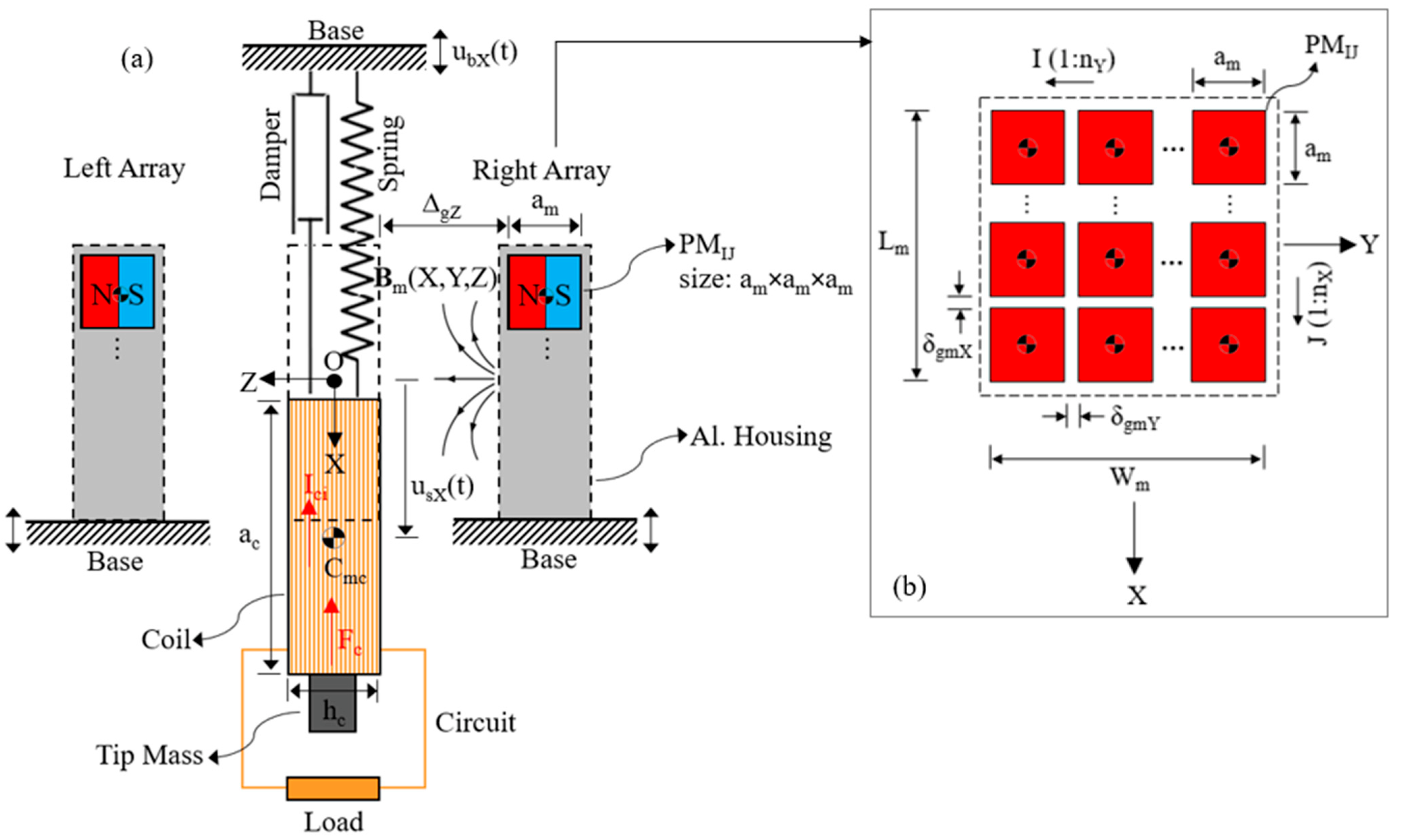
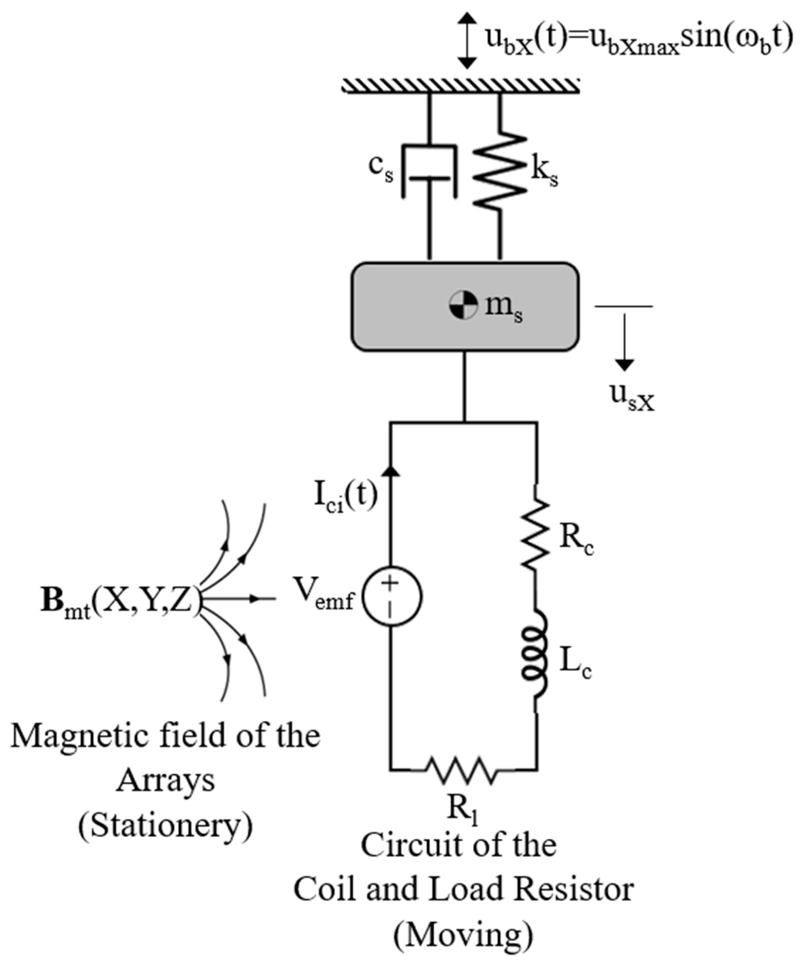
2. Mathematical Modeling of EMEHs

An electromechanical model is presented to evaluate the performance of an EMEH with planar arrays to harvest electrical energy from the traffic-induced vibration of highway bridges. Figure 1 illustrates the configuration of the EMEH consisting of a thick rectangular copper coil moving relative to two identical planar arrays of permanent magnets (PMs) located on its left and right sides. The magnetic arrays are firmly fastened to a base moving with the displacement u_bX(t) along the X-axis. They are mounted inside two housings made of a non-magnetic material such as aluminum. The coil is attached to the base through a system of elastic springs and viscous dampers. The size of the vertical air gap between the coil and the left and right arrays along the Z-axis is denoted by Δ_gZ. This is an important parameter that controls the strength of magnetic interactions between the arrays and the coil.

Figure 1b shows the plan of the left and right arrays in the XY-plane. Each array consists of n = n_X × n_Y cuboidal PMs of the size a_m × a_m × a_m which are separated from each other through air gaps of the size δ_gmX and δ_gmY along the X- and Y-axes, respectively. Therefore, the dimensions of the left and right arrays would be L_m = n_Xa_m + (n_X − 1)δ_gmX, W_m = n_Ya_m + (n_Y − 1)δ_gmY, and H_m = a_m.

Electrical power is harvested from the EMEH by connecting the coil to a series electrical load representing the resistance of the harvesting circuit. The harvested electrical power is generated by the electromagnetic induction occurring in the coil when it moves relative to the left and right arrays. The motion of the coil results in a change in the magnetic flux of PMs inducing an electromotive force in the coil according to Faraday’s law. This results in the electric current I_ci(t) flowing in the copper wire of the coil whose direction varies with the motion of the coil. The direction of this electric current changes as per Lenz’s law in such a way that the induced magnetic field opposes the initial cause of change in the magnetic flux of the PMs, which is the motion of the coil. Eventually, this interaction causes the braking (damping) force F_c that acts on the coil and its direction which is always opposite to the direction of the velocity of the coil, i.e., ${\stackrel{\text{⋅}}{\mathrm{u}}}_{\mathrm{sX}}\left(\mathrm{t}\right)$.

2.1. Electromechanical Model

The EMEH can be modeled as a linear single-degree-of-freedom (SDOF) system coupled with a series alternating-current RL circuit as shown in Figure 2. The SDOF system is subjected to the base excitation u_bX(t) = u_bXmaxsin(ω_bt) along the X-axis where u_bXmax and ω_b = 2πf_b are the amplitude and the circular frequency of the excitation, and f_b is the frequency of the excitation. The stiffness and mechanical damping coefficients of the elastic spring and viscous damper are denoted by k_s and c_s, respectively. The total mass of the SDOF system, consisting of the mass of the coil and the tip mass, is denoted by m_s. The degree of freedom of the SDOF system is also denoted by u_sX which represents the displacement of the mass center of the coil.

The RL circuit consists of two resistors, R_c and R_l, and an inductor L_c connected in series to an altering-voltage source with the electromotive force V_emf. R_c and L_c represent the resistance and induction of the coil, respectively, and R_l is the resistance of the electrical load used to harvest the electrical power.

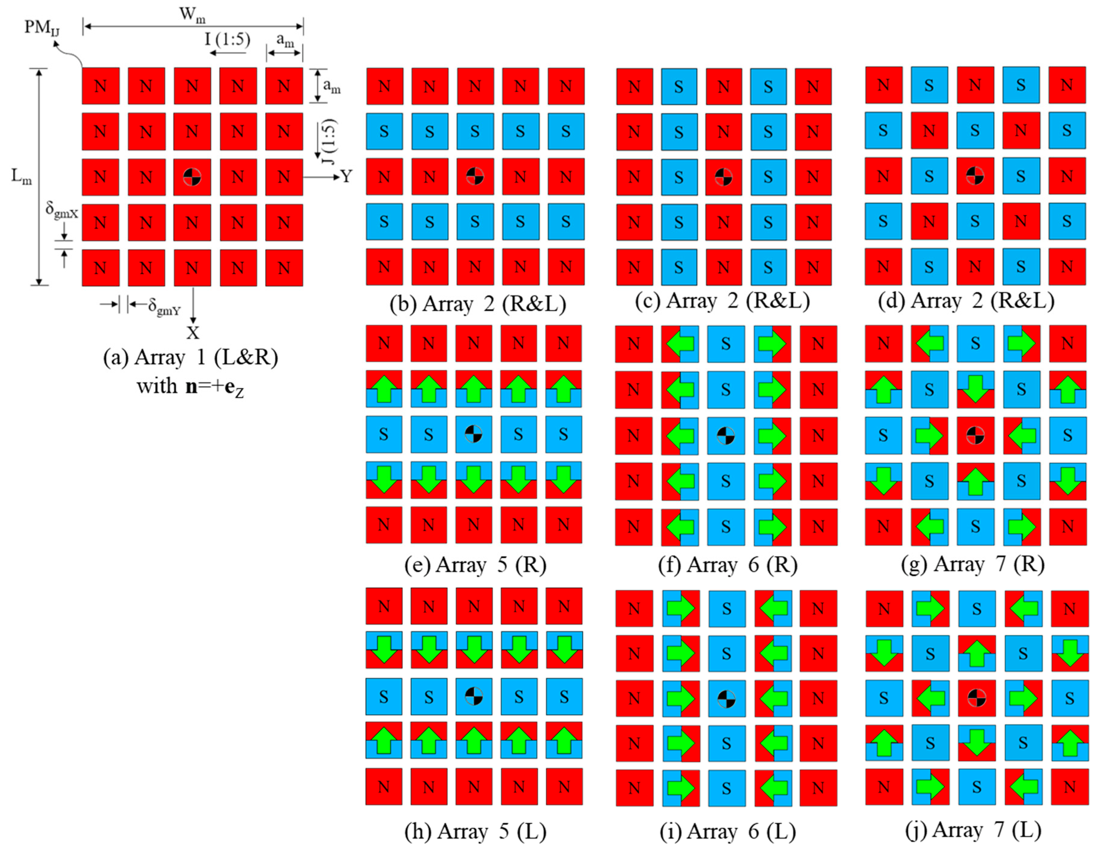
2.2. Planar Arrangement of the PMs

The arrangement of the PMs based on the direction of their poles is an important feature of the EMEH that can significantly affect the magnetic interaction of the PMs with the coil. Figure 3 shows the planar arrangement of the PMs poles in seven different multipole arrays including: (1) uniform, (2) X-linear alternating, (3) Y-linear alternating, (4) planar alternating, (5) X-linear Halbach, (6) Y-linear Halbach, and (7) planar Halbach arrays. It is assumed that n_X = 5 and n_Y = 5 in this study as n = 5 is the minimum number of PMs required to create a linear Halbach array. These arrays, therefore, consist of 25 identical cubic PMs with the side length a_m, which are separated from each other by air gaps of the size δ_gmX and δ_gmY along the X- and Y-axes, respectively.

From Figure 3 it is observed that Arrays 3 and 6 are created by rotating Arrays 2 and 5 through an angle of 90°, respectively. However, it should be noted that the magnetic interaction of the coil with these arrays are different compared to that with Arrays 2 and 5. This is because the angle that the magnetic flux density vectors of these arrays make with the direction of motion are different compared to Arrays 2 and 5, and this feature can change the strength of induced electric current quite significantly [6,7].

The magnetic flux density vector of IJ-th PM in an array is given by the following surface integral obtained from the solution of magnetostatic form of Maxwell’s equations governing the magnetic field of the PM [6],

$$B_{\mathrm{mIJ}}=\frac{{\mathsf{\mu }}_0}{4\mathsf{\pi }}{{\displaystyle \iint }}_{{\mathrm{S}}_{\mathrm{m}\mathrm{IJ}}}\left(M_{\mathrm{rmIJ}}\times n\right)\times \frac{r-r_0}{{\left|r-r_0\right|}^3}{\mathrm{dS}}_0$$

(1a)

where n is the unit surface normal vector, $M_{\mathrm{rmIJ}}=\left({\mathsf{\gamma }}_{\mathrm{XIJ}}{e}_{\mathrm{X}}+{\mathsf{\gamma }}_{\mathrm{YIJ}}{e}_{\mathrm{Y}}+{\mathsf{\gamma }}_{\mathrm{ZIJ}}{e}_{\mathrm{Z}}\right){\mathrm{B}}_{\mathrm{rmIJ}}/{\mathsf{\mu }}_0$ is the magnetization vector of PM in which ${\mathsf{\gamma }}_{\mathrm{XIJ}}$, ${\mathsf{\gamma }}_{\mathrm{YIJ}}$, and ${\mathsf{\gamma }}_{\mathrm{ZIJ}}$ are constants showing the direction of vector, B_rmIJ is the magnetic remanence, and r and r₀ are the position vectors of field and source points, respectively. Note that μ₀ = 4π × 10⁻⁷ Tm/A is the magnetic permeability of the vacuum.

By solving this integral, the magnetic flux density vector of each of the left B_mla(X,Y,Z) and right B_mra(X,Y,Z) arrays shown in Figure 2a can be calculated by summing up the magnetic flux density vectors of the PMs,

$$B_{\mathrm{ma}}\left(\mathrm{X},\mathrm{Y},\mathrm{Z}\right)={\displaystyle \sum }_{\mathrm{I}=1}^{{\mathrm{n}}_{\mathrm{Y}}}{\displaystyle \sum }_{\mathrm{J}=1}^{{\mathrm{n}}_{\mathrm{X}}}{B}_{\mathrm{mIJ}}$$

(1b)

where B_mIJ is given by

$$B_{\mathrm{mIJ}}=-\frac{1}{4\mathsf{\pi }}{\displaystyle \sum }_{\mathrm{i},\mathrm{j},\mathrm{k}=1}^2{(-1)}^{\mathrm{i}+\mathrm{j}+\mathrm{k}}{M}_{\mathrm{rmIJ}}\cdot b\left(\mathrm{X}-{\mathrm{X}}_{\mathrm{cIJi}},\mathrm{Y}-{\mathrm{Y}}_{\mathrm{cIJj}},\mathrm{Z}-{\mathrm{Z}}_{\mathrm{cIJk}}\right)$$

(1c)

where b is a 2nd order tensor function in space defined as

$$b(\mathrm{X},\mathrm{Y},\mathrm{Z})=\left[\begin{array}{ccc}{\tan }^{-1}\left[\frac{\mathrm{YZ}}{\mathrm{XR}}\right]& \ln [\mathrm{Z}+\mathrm{R}]& \ln [\mathrm{Y}+\mathrm{R}]\\ \ln [\mathrm{Z}+\mathrm{R}]& {\tan }^{-1}\left[\frac{\mathrm{XZ}}{\mathrm{YR}}\right]& \ln [\mathrm{X}+\mathrm{R}]\\ \ln [\mathrm{Y}+\mathrm{R}]& \ln [\mathrm{X}+\mathrm{R}]& {\tan }^{-1}\left[\frac{\mathrm{XY}}{\mathrm{ZR}}\right]\end{array}\right]$$

(1d)

in which R = (X² + Y² + Z²)^1/2. Furthermore, in Equation (1c), X = X_cIJ1, X = X_cIJ2, Y = Y_cIJ1, Y = Y_cIJ2, Z = Z_cIJ1, and Z = Z_cIJ2 are the coordinates of boundary surfaces surrounding the volume of IJ-th PM on the X-, Y-, and Z-axes, respectively.

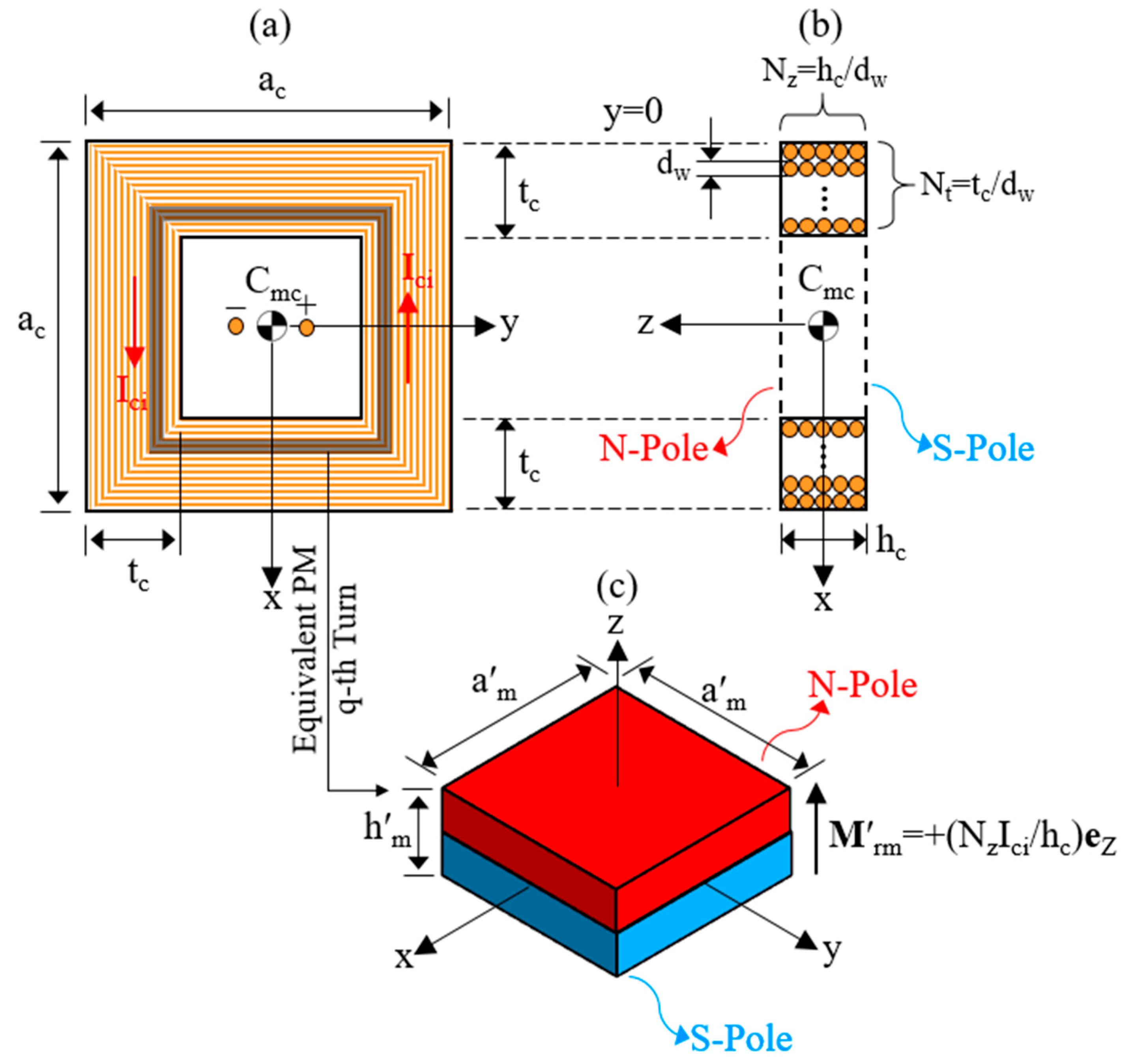
2.3. Thick Rectangular Coil

Figure 4a,b show the horizontal and vertical cross-sections of the coil with an air core including its key geometrical parameters. The length of coil is a_c, the width is a_c, the height is h_c, and the winding depth is t_c. In this figure, N_z = h_c/d_w and N_t = t_c/d_w denote the numbers of turns along the z-axis and the depth of winding, respectively, where d_w is the diameter of the winding wire. Therefore, the total number of turns can be calculated as N_c = N_z × N_t. It is assumed that when the electric current I_ci(t) is counterclockwise in the xy-plane, I_ci(t) is positive. This implies that the N- and S-poles are established at z = +h_c/2 and z = −h_c/2, respectively.

A single-layer turn coil with the surface current density K′_bm is modeled by an equivalent PM of the same dimensions as shown in Figure 4c. The magnetization vector M′_rm of the equivalent PM is related to K′_bm through K′_bm = M′_rm × n, where n is the unit surface normal vector of the equivalent PM [32]. The shell method [33] can be used to model a multi-layer turn coil referred to as the thick rectangular coil in this study. This method treats each single layer of turn as an equivalent cuboidal PM of the dimension a′_mq × a′_mq × h′_mq where a′_mq = a_c−[2(N_t − q) − 1]d_w and h′_mq = h_c. The magnetic remanence of this PM is B′_rm = μ₀(N_zI_ci/h_c) where B′_rm = μ₀M′_rm and I_ci = (h_cK′_bm)/N_z.

The magnetic field of the coil can be calculated by superposing the magnetic fields of all the equivalent cuboidal PMs as follows,

$$B_{\mathrm{c}}\left(\mathrm{X},\mathrm{Y},\mathrm{Z}\right)={\displaystyle \sum }_{\mathrm{q}=1}^{{\mathrm{N}}_{\mathrm{t}}}{B}_{\mathrm{cq}}$$

(2)

where B_cq is the magnetic flux density vector of the q-th turn of the coil that is calculated by Equation (1) for n_X = n_Y = 1 as per the shell method [33].

The resistance of the coil is given by

$${\mathrm{R}}_{\mathrm{c}}=\frac{{\mathrm{l}}_{\mathrm{w}}}{{\mathsf{\sigma }}_{\mathrm{c}}{\mathrm{A}}_{\mathrm{w}}}$$

(3)

in which l_w = 4N_zN_t(a_c − t_c), σ_c = 58.58 MS/m, and ${\mathrm{A}}_{\mathrm{w}}={\mathsf{\pi }\mathrm{d}}_{\mathrm{w}}^2/4$ are the length, electrical conductivity, and cross-section area of the winding copper wire, respectively. The inductance of the coil is also given by [34],

$${\mathrm{L}}_{\mathrm{c}}=2\frac{{\mathsf{\mu }}_0}{\mathsf{\pi }}{\mathrm{N}}_{\mathrm{z}}^2{\displaystyle \sum }_{\mathrm{q}=1}^{{\mathrm{N}}_{\mathrm{t}}}{\mathrm{a}}_{\mathrm{cq}}\left[\ln \left(\frac{{\mathrm{a}}_{\mathrm{cq}}}{{\mathrm{d}}_{\mathrm{w}}}\right)-0.0809\right]$$

(4)

where a_cq = a_c − 2(N_t − q)d_w is the length of the sides of q-th turn.

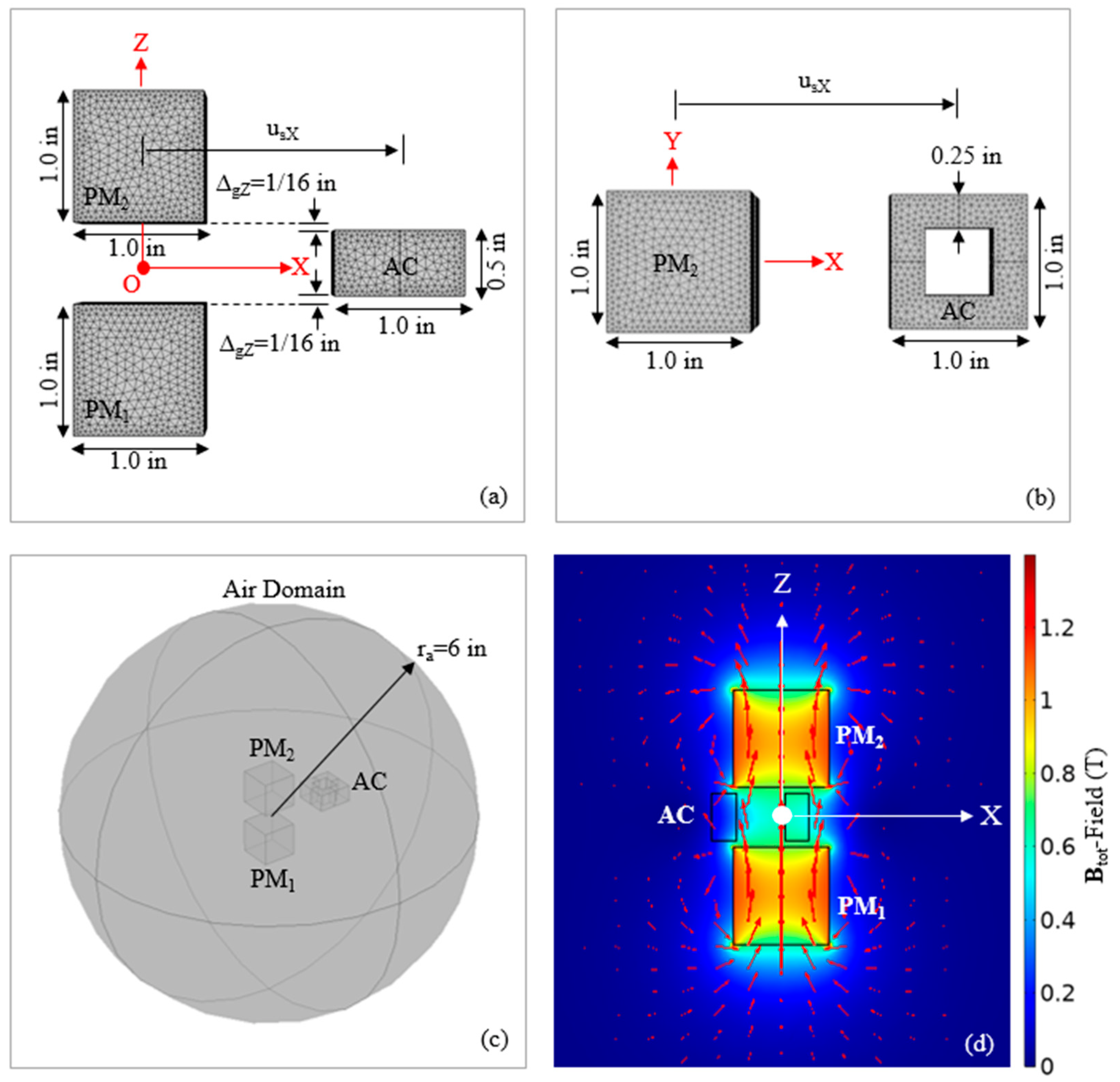
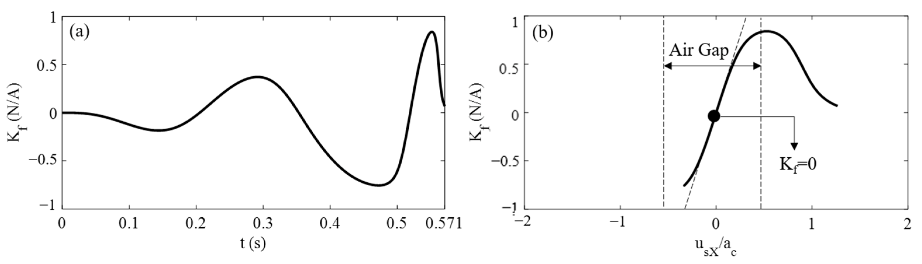
2.4. Magnetic Interaction of the Arrays with the Moving Coil

The X-component of magnetic force acted on the moving coil when subjected to the magnetic field of each array is given by

$${\mathrm{F}}_{\mathrm{cX}}={\displaystyle \sum }_{\mathrm{I}=1}^{{\mathrm{n}}_{\mathrm{Y}}}{\displaystyle \sum }_{\mathrm{J}=1}^{{\mathrm{n}}_{\mathrm{X}}}{\mathrm{F}}_{\mathrm{cXIJ}}$$

(5a)

where F_cXIJ is the magnetic force applied to the coil due to the magnetic field of IJ-th PM. This force can be computed by the shell method as follows [33],

$${\mathrm{F}}_{\mathrm{cXIJ}}={\displaystyle \sum }_{\mathrm{q}=1}^{{\mathrm{N}}_{\mathrm{t}}}{\mathrm{F}}_{\mathrm{mXIJq}}^{\prime }$$

(5b)

where F′_mXIJq is the magnetic force applied to the q-th turn of the coil due to the magnetic field of the IJ-th PM and is given by [6,7],

$${\mathrm{F}}_{\mathrm{mXIJq}}^{\prime }=\frac{1}{16{\mathsf{\pi }\mathsf{\mu }}_0}{\mathrm{B}}_{\mathrm{rmIJ}}{\mathrm{B}}_{\mathrm{rm}}^{\prime }{{\mathrm{V}}^{\prime }}_{\mathrm{mq}}^{\frac{2}{3}}{\mathrm{f}}_{\mathrm{mXIJq}}^{\prime }\left({\mathsf{\alpha }}_{\mathrm{mq}}^{\prime },{\mathsf{\gamma }}_{\mathrm{mq}}^{\prime },{\mathsf{\beta }}_{\mathrm{mq}}^{\prime },\frac{{\mathsf{\Delta }\mathrm{X}}_{\mathrm{mIJq}}^{\prime }}{{\mathrm{a}}_{\mathrm{mq}}^{\prime }},\frac{{\mathsf{\Delta }\mathrm{Y}}_{\mathrm{mIJq}}^{\prime }}{{\mathrm{a}}_{\mathrm{mq}}^{\prime }},\frac{{\mathsf{\Delta }\mathrm{Z}}_{\mathrm{mIJq}}^{\prime }}{{\mathrm{h}}_{\mathrm{mq}}^{\prime }}\right)$$

(5c)

where V′_mq is the volume of the equivalent cuboidal PM enclosed by the q-th turn of the coil and fʹ_mXIJq(.) is a dimensionless function in term of surface integrals carried over the equivalent cuboidal PM [7]. This function depends on the following parameters: (i) the aspect ratio of the turn α′_mq = a′_mq/h′_mq in which a′_mq=a_c − (2q − 1)d_w and h′_mq = h_c; (ii) the geometrical ratios ${\mathsf{\gamma }}_{\mathrm{mq}}^{\prime }={\mathrm{a}}_{\mathrm{m}}/{\mathrm{a}}_{\mathrm{mq}}^{\prime }$ and ${\mathsf{\beta }}_{\mathrm{mq}}^{\prime }={\mathrm{a}}_{\mathrm{m}}/{\mathrm{h}}_{\mathrm{mq} }^{\prime }$and (iii) the mass center eccentricity ratios ΔX_mIJq/a′_mq, ΔY_mIJq/a′_mq, and ΔZ_mIJq/h′_mq along the X-, Y-, and Z-axes, respectively, where Δ(.)′_mIJq = (.)_mIJ−(.)′_mq.

3. Electromechanical Equation

The motion of the coil when subjected to the magnetic field of the left and right arrays with the total magnetic flux density vector field B_mta = B_mla(X, Y, Z) + B_mra(X, Y, Z) is described by the following two-degrees-of-freedom coupled electromechanical equation:

$${\mathrm{m}}_{\mathrm{s}}{\ddot{\mathrm{u}}}_{\mathrm{sX}}\left(\mathrm{t}\right)+{\mathrm{c}}_{\mathrm{s}}{\stackrel{\text{⋅}}{\mathrm{u}}}_{\mathrm{sX}}\left(\mathrm{t}\right)+{\mathrm{k}}_{\mathrm{s}}{\mathrm{u}}_{\mathrm{sX}}\left(\mathrm{t}\right)-{\mathrm{F}}_{\mathrm{ctX}}\left(\mathrm{t}\right)=-{\mathrm{m}}_{\mathrm{s}}{\ddot{\mathrm{u}}}_{\mathrm{bX}}\left(\mathrm{t}\right)$$

(6a)

$$\left({\mathrm{R}}_{\mathrm{l}}+{\mathrm{R}}_{\mathrm{c}}\right){\mathrm{I}}_{\mathrm{ci}}\left(\mathrm{t}\right)+{\mathrm{L}}_{\mathrm{c}}{\stackrel{\text{⋅}}{\mathrm{I}}}_{\mathrm{ci}}\left(\mathrm{t}\right)={\mathrm{V}}_{\mathrm{emf}}\left(\mathrm{t}\right)$$

(6b)

where F_ctX is the X-component of the total magnetic force applied to the coil, i.e., F_ct = F _cla+F_cra in which F_cla and F_cra are calculated by Equation (5a–c). In Equation (6a), ${\ddot{\mathrm{u}}}_{\mathrm{bX}}\left(\mathrm{t}\right)={\ddot{\mathrm{u}}}_{\mathrm{bXmax}}\sin ({\mathsf{\omega }}_{\mathrm{b}}\mathrm{t})$ in which ${\ddot{\mathrm{u}}}_{\mathrm{bXmax}}={\mathrm{u}}_{\mathrm{bXmax}}{\mathsf{\omega }}_{\mathrm{b}}^2$ is the maximum acceleration of the base.

3.1. Decoupled Equation of Motion

Equations (6a) and (6b) are coupled in the current form. They can, however, be decoupled and written into one single equation by finding the relationship between F_ctX and V_emf as discussed below.

The magnetic force F_ctX can be alternatively calculated by the Lorentz’s formula for a current-carrying wire in electromagnetism as follows,

$${\mathrm{F}}_{\mathrm{ctX}}={\mathrm{I}}_{\mathrm{ci}}{{\displaystyle \oint }}_{\mathrm{coil}}\left(\mathrm{d}l\times B_{\mathrm{mt}}\right)·e_{\mathrm{X}}$$

(7a)

where the line integration is taken over the total length of the copper wire while moving in the magnetic field of the arrays. Here, it should be noted that the direction of this force is always opposite to the direction of the velocity of the coil, i.e., F_ctX = −c_e${\stackrel{\text{⋅}}{\mathrm{u}}}_{\mathrm{sX}}$ where c_e is the electrical damping caused by the magnetic interaction between the coil and the arrays. The correct sign of this force is implicit in Equation (7a). This force can be written in the following simple form,

$${\mathrm{F}}_{\mathrm{ctX}}=-{\mathrm{K}}_{\mathrm{f}}{\mathrm{I}}_{\mathrm{ci}}$$

(7b)

where K_f is called electromechanical coupling coefficient or transformation factor [17] which is defined by

$${\mathrm{K}}_{\mathrm{f}}={{\displaystyle \oint }}_{\mathrm{coil}}\left(B_{\mathrm{mt}}\times \mathrm{d}l\right)·e_{\mathrm{X}}.$$

(8)

This coefficient is time-varying because the limits of integration in Equation (8) vary with the motion of coil. K_f can be calculated by Equation (5) for I_ci = −1 A because according to Equation (7b) as K_f = F_ctX for I_ci = −1 A.

Many researchers (For example see: [2,18,35,36]) have assumed that K_f is constant and does not change with time. That is, they have assumed that K_f = N_zB_mtavg(a_c − t_c) where B_mtavg is the volume average of the magnetic flux density vector of the left and right arrays over the air gap between them. This is an oversimplified assumption that can result in error when estimating the harvested electrical power [35,36]. This error is lowest for thin copper coils placed in a narrow air gap.

The electromotive force V_emf can be calculated by the following integral taken over the length of the coil,

$${\mathrm{V}}_{\mathrm{emf}}={\stackrel{\text{⋅}}{\mathrm{u}}}_{\mathrm{sX}}\left[{{\displaystyle \int }}_{\mathrm{coil}}\left(e_{\mathrm{X}}\times B_{\mathrm{ext}}\right)·\mathrm{d}l\right].$$

(9a)

By comparing the triple product under the integral and comparing it with Equation (8), it can be concluded that,

$${\mathrm{V}}_{\mathrm{emf}}=+{\mathrm{K}}_{\mathrm{f}}{\stackrel{\text{⋅}}{\mathrm{u}}}_{\mathrm{sX}}$$

(9b)

which shows that the generation of the induced alternating voltage in the coil is coupled to the velocity of the coil and its magnetic interaction with the left and right arrays. Therefore, the relationship between the induced electric current I_ci = V_emf/(R_l + R_c) and the velocity of the coil can be obtained as

$${\mathrm{I}}_{\mathrm{ci}}=\frac{{\mathrm{K}}_{\mathrm{f}}}{{\mathrm{R}}_{\mathrm{l}}+{\mathrm{R}}_{\mathrm{c}}}{\stackrel{\text{⋅}}{\mathrm{u}}}_{\mathrm{sX}}.$$

(10)

This equation can be used to simplify the governing equation by eliminating I_ci from Equation (6a) as follows:

$${\ddot{\mathrm{u}}}_{\mathrm{sX}}\left(\mathrm{t}\right)+2{\mathsf{\omega }}_{\mathrm{s}}\left[{\mathsf{\xi }}_{\mathrm{s}}+\frac{{\mathrm{K}}_{\mathrm{f}}{\left(\mathrm{t}\right)}^2}{2{\mathrm{m}}_{\mathrm{s}}{\mathsf{\omega }}_{\mathrm{s}}\left({\mathrm{R}}_{\mathrm{l}}+{\mathrm{R}}_{\mathrm{c}}\right)}\right]{\stackrel{\text{⋅}}{\mathrm{u}}}_{\mathrm{sX}}\left(\mathrm{t}\right)+{\mathsf{\omega }}_{\mathrm{s}}^2{\mathrm{u}}_{\mathrm{sX}}\left(\mathrm{t}\right)={\ddot{\mathrm{u}}}_{\mathrm{bXmax}}\sin ({\mathsf{\omega }}_{\mathrm{b}}\mathrm{t})$$

(11)

in which ξ_s is the critical mechanical damping ratio. The average electrical power harvested from the EMEH over the time interval [0,τ] is given by

$${\mathrm{P}}_{\mathrm{lavg}}=\frac{1}{\mathsf{\tau }}{{\displaystyle \int }}_0^{\mathsf{\tau }}{\mathrm{P}}_{\mathrm{l}}\left(\mathrm{t}\right)\mathrm{dt}$$

(12a)

in which P_l is the instantaneous power consumed by the load which is given by

$${\mathrm{P}}_{\mathrm{l}}=\frac{{\mathrm{R}}_{\mathrm{l}}}{{\left({\mathrm{R}}_{\mathrm{l}}+{\mathrm{R}}_{\mathrm{c}}\right)}^2}{\mathrm{K}}_{\mathrm{f}}^2{\stackrel{\text{⋅}}{\mathrm{u}}}_{\mathrm{sX}}^2.$$

(12b)

3.2. Numerical Verification

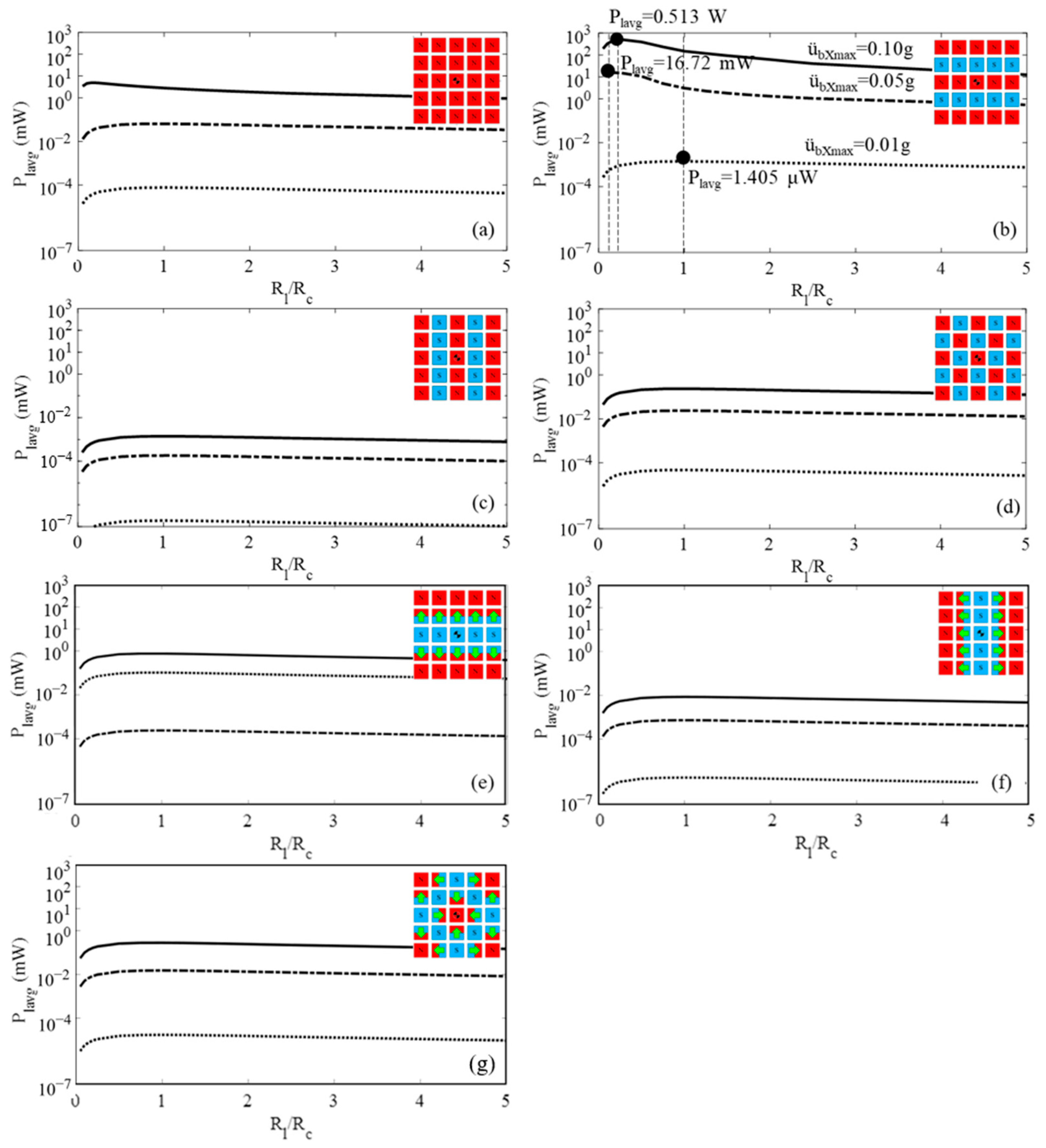
A 3D finite element (FE) model of a simple EMEH is developed in COMSOL Multiphysics software [37] to verify the accuracy of proposed analytical method, i.e., Equations (5a–c) and (7a,b). The FE model consists of a coil located in the vicinity of two identical PMs. The coil has the dimensions of 1 in × 1 in × 0.5 in, and the winding depth t_c = 0.25 in, wound by a copper wire of 18-AWG with d_w ≅ 1 mm and the ampacity current 16 A [38]. The two PMs are identical with the dimensions 1 in × 1 in × 0.5 in and the magnetic remanence B_rm = 1.4 T (neodymium type N52). The size of the vertical gap between the coil and the PMs is ∆_gcZ = 0.25 in.

Figure 5a,b shows this model and the details of the meshing. A sphere of the radius r_a = 6 in. is used to model the air domain enclosing the PMs and coil. The center of this sphere is located at the center of air gap between the PMs where the origin of XYZ coordinate system is located.

Table 1. Geometrical and material parameters of the coil and PMs in the FE model developed in COMSOL Multiphysics software.

Parameter	Value	Unit	Description
am	1	in	Length of the sides of the PMs
ac	1	in	Length of the sides of the coil
hc	0.5	in	Height of the coil (Nz = 13)
tc	0.25	in	Winding depth (Nt = 6)
dw	1	mm	Diameter of the copper wire (18-AWG)
ΔgcZ	1/16	in	Size of the vertical gap between the coil and the PMs
Brm	1.4	T	Magnetic remanence of the PMs (Neodymium, type N52)
σc	58.58	MS/m	Electrical conductivity of copper wire

shows the geometrical and material parameters of the FE model.

The problem set up here is stationary, implying that the electric current flowing through the coil, denoted by I_ci, is not time-dependent. Therefore, the attractive magnetic interaction between the coil and the PMs can be described by the magnetostatic form of the Maxwell equations in the presence of an external current as follows [32],

$$\begin{array}{ccc}\nabla \times \left(\frac{1}{{\mathsf{\mu }}_{\mathrm{m}}}\nabla \times A\right)=J_{\mathrm{e}}& ,& B_{\mathrm{mt}}=\nabla \times A\end{array}$$

(13)

where A is the magnetic vector potential, J_e is the volume density vector of the electric current, and μ_m is the magnetic permeability of the materials including the PMs (μ_m ≅ μ₀) and air domain (μ_m = μ₀).

Equation (13) is solved by a stationary solver in COMSOL Multiphysics software [37]. To solve this equation, the magnetic insulation boundary condition and the equation ∇•A = 0 (Coulomb gauge) must be satisfied. The Maxwell stress tensor is also used to calculate the magnetic force applied to the coil [6,7,39]. It is important to employ a very fine mesh along the edges of coil and PMs to make sure that the results are accurate, as illustrated in Figure 5a,b.

Figure 5d shows the magnetic flux density field of the PMs on the XZ-plane at Y = 0 calculated by the FE model for u_sX = −0.216a_c and I_ci = −0.849 A. The magnetic flux density field of the AC is negligible.

The SDOF system is subjected to the base excitation ü_bX(t) = ü_bXmaxsin(ω_bt) along the X-axis with ü_bXmax = 0.05 g, f_b = 3.5 Hz, and 0 ≤ t ≤ 2T_b where T_b = 1/f_b = 0.286 s.

Table 2. Parameters of the SDOF model developed in MATLAB.

Parameter	Value	Unit	Description
fb	3.5	Hz	Frequency of the base excitation
übXmax	0.05 g	m/s2	Maximum acceleration of the base excitation (ubXmax = übXmax/ωb2 = 15.2 cm)
fs	3.5	Hz	Frequency of the SDOF system
ξs	5	%	Critical mechanical damping ratio of the SDOF system
ms	41.8	gr	Mass of the SDOF system (ms = mw = 41.8 gr)
Rc	129	mΩ	Resistance of the coil
Rl	129	mΩ	Resistance of the electrical load (Rl/Rc = 1)

shows parameters of the SDOF model. The motion of this system is described by Equation (11). A numerical solver is used in MATLAB [40] to solve this equation.

Time histories of the displacement of coil, the magnetic force applied to the coil, and the induced electric current are shown in Figure 6a–c, respectively. First, for given values of u_sX and I_ci, we calculate the magnetic force by using the analytical model. Then it is compared to the corresponding value resulting from the FE model.

The FE model is used to calculate the magnetic force for the displacements u_sX = −0.199a_c and +0.733a_c and the currents I_ci = −0.550 and +2.782 A, respectively, assuming a_c=1 in. These values have been shown on Figure 6a,b with points 1 and 2, respectively. The results have been compared to those obtained from the analytical model as can be observed on Figure 6c. It is seen that there is a good agreement between the analytical and FE models. This validates the accuracy of the proposed analytical method in this paper.

Figure 7a shows the time history of the electromechanical coupling coefficient. Figure 7b also shows the variation of this coefficient with the displacement of the coil. It is seen that K_f is maximum at u_sX = ±0.5a_c and very low at large displacements; approximately beyond two times of the length of the air gap along the X-axis where the mechanical energy domain is totally decoupled from the electromagnetic energy domain.

4. Parametric Study

The maximum average electrical power is calculated numerically by solving Equation (11) in MATLAB due to the time-varying nature of the electromechanical coupling coefficient. A parametric analysis is carried out to find the optimal load resistance of EMEH for three different intensity levels of the base excitation. For this purpose, the SDOF system is subjected to the base excitation ü_bX(t) = ü_bXmaxsin(ω_bt) along the X-axis for ü_bXmax = 0.01 g, 0.05 g, and 0.10 g and f_b = 3.5 Hz over the time interval 0 ≤ t ≤ 2 T_b where T_b = 1/f_b = 0.286 s. The EMEH is tuned to undergo the resonant condition with the frequency f_s = f_b = 3.5 Hz.

Table 3. Electromechanical parameters of the EMEH.

Parameter	Value	Unit	Description
am	0.5	in	Length of the sides of the PMs
δgmX	1	mm	Size of the gap between the PMs along the X-axis
δgmY	1	mm	Size of the gap between the PMs along the Y-axis
nX	5		Number of the PMs along the X-axis
nY	5		Number of the PMs along the Y-axis
ac	2.5	in	Length of the sides of the coil
hc	0.5	in	Height of the AC (Nz = 13)
tc	0.5	in	Winding depth (Nt = 13)
dw	1	mm	Diameter of the copper wire (18-AWG)
ΔgcZ	1/16	in	Size of the vertical gap between the coil and the PMs
Brm	1.4	T	Magnetic remanence of the PMs
σc	58.58	MS/m	Electrical conductivity of copper wire
fb	3.5	Hz	Frequency of the base excitation
übXmax	Var.	m/s2	Maximum acceleration of the base excitation
fs	3.5	Hz	Frequency of the SDOF system (fs = fb)
ξs	5	%	Critical mechanical damping ratio of the SDOF system
ms	241.7	gr	Mass of the SDOF system (ms = mw)
Rc	746.4	mΩ	Resistance of the coil
Rl	Var.	mΩ	Resistance of the electrical load

shows the electromechanical parameters of the EMEH.

Figure 8a–g shows the variation of the average electrical power versus the ratio of the load resistance to that of the coil R_l/R_c for Array 1, 2, …, and 7. It is seen that the EMEH can deliver the highest electrical power when the PMs are arranged according to Array 2 in which the poles alternate along the X-axis. The average electrical power increases with the increase of the intensity of the base acceleration. It is seen that for ü_bXmax = 0.1 g the maximum average electrical power is equal to P_lavgmax = 513 mW that can be delivered by the load resistance R_lopt = 0.25 R_c = 186.6 mΩ. The amount of power is relatively very large and can be uses to power conventional sensors used for structural health monitoring of bridges. Larger amounts of electrical power can be delivered by adding a greater number of coils and having arrays installed in parallel.

It is seen that the optimal load resistance is smaller than the coil resistance R_lopt < R_c as shown in Figure 8b. However, this is not the case when the electrotechnical coefficient is assumed to be constant. The maximum average electrical power can be calculated by putting the derivative of P_lavg with respect to R_l equal to zero that results in the calculation of the optimal load resistance as follows [41],

$${\mathrm{R}}_{\mathrm{lopt}}={\mathrm{R}}_{\mathrm{c}}+\frac{{\mathrm{K}}_{\mathrm{f}}^2}{2{\mathsf{\xi }}_{\mathrm{s}}{\mathrm{m}}_{\mathrm{s}}{\mathsf{\omega }}_{\mathrm{b}}}.$$

(14)

This shows that R_lopt > R_c when K_f is assumed to be constant. This approach to the calculation of the maximum average electrical power is, however, not accurate due to the assumption that K_f is constant as used in a large number of previous research works [2,18,42,43,44].

5. Experimental Study

A proof-of-concept prototype is designed and fabricated for laboratory and field testing of the EMEH with planar magnetic arrays. Figure 9 shows this prototype of the EMEH designed and fabricated for the purpose of proof-of-concept testing in both the laboratory and field environments. The configuration of the prototype is based on the design and finite element simulation developed in the previous section with slight differences in the size of the coil. The prototype consists of an aluminum plate of the size 10 × 10 × 0.25 in used as the base plate to transfer the base excitation; four springs with the total stiffness coefficient 825 N/m; an aluminum plate of the size 8 × 3 × 0.25 in used to hold a total mass of m_s = 0.49 kg on the springs; a rectangular copper coil with a thickness of 0.25 in and the outside size 2.25 × 2.25 in and the inside size 1.75 × 1.75 in, two magnetic arrays consisting of 25 cubic neodymium PMs of the size 0.5 × 0.5 × 0.5 in with the magnetic remanence of B_rm = 1.2 T (neodymium, type N42). The frequency of the system was estimated to be approximately about f_s = 6.5 Hz.

It should be noted that, for the sake of fabrication simplicity, the PMs have been arranged according to Array 4 in Figure 3. The PMs in this array are in a static force-equilibrium condition that facilitates their arrangement with bare hands. This array causes a lower output voltage compared to Array 2, which has strongest magnetic interaction with the coil as illustrated in Figure 8. The PMs in each one of the left and right magnetic arrays are arranged in such a way that their opposing poles face the PMs in the other array. This strengthens the flow of magnetic flux between the two arrays when passing through the coil as shown in Figure 9.

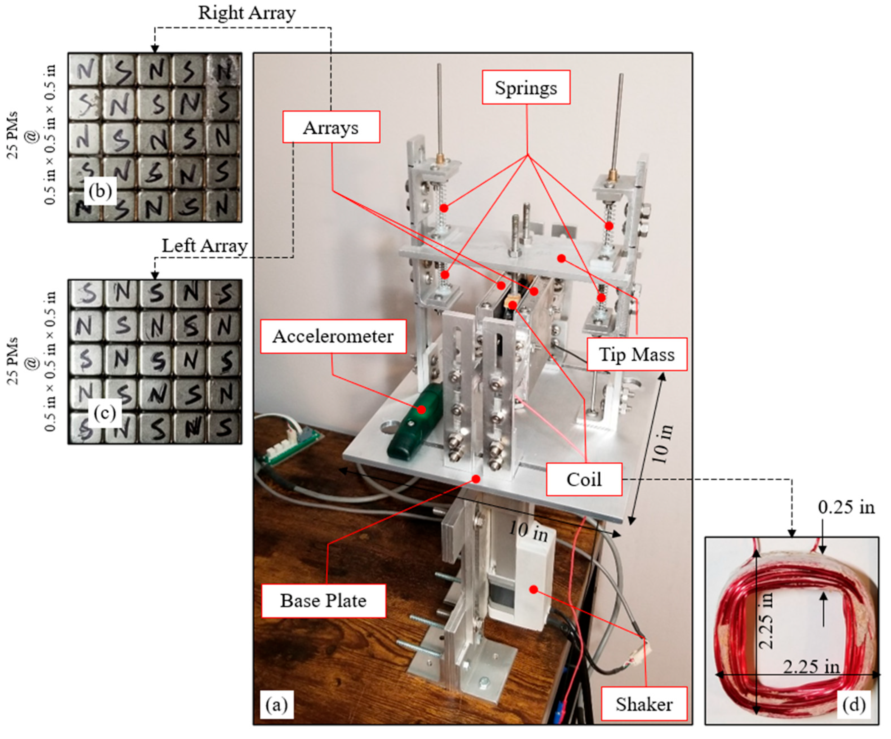
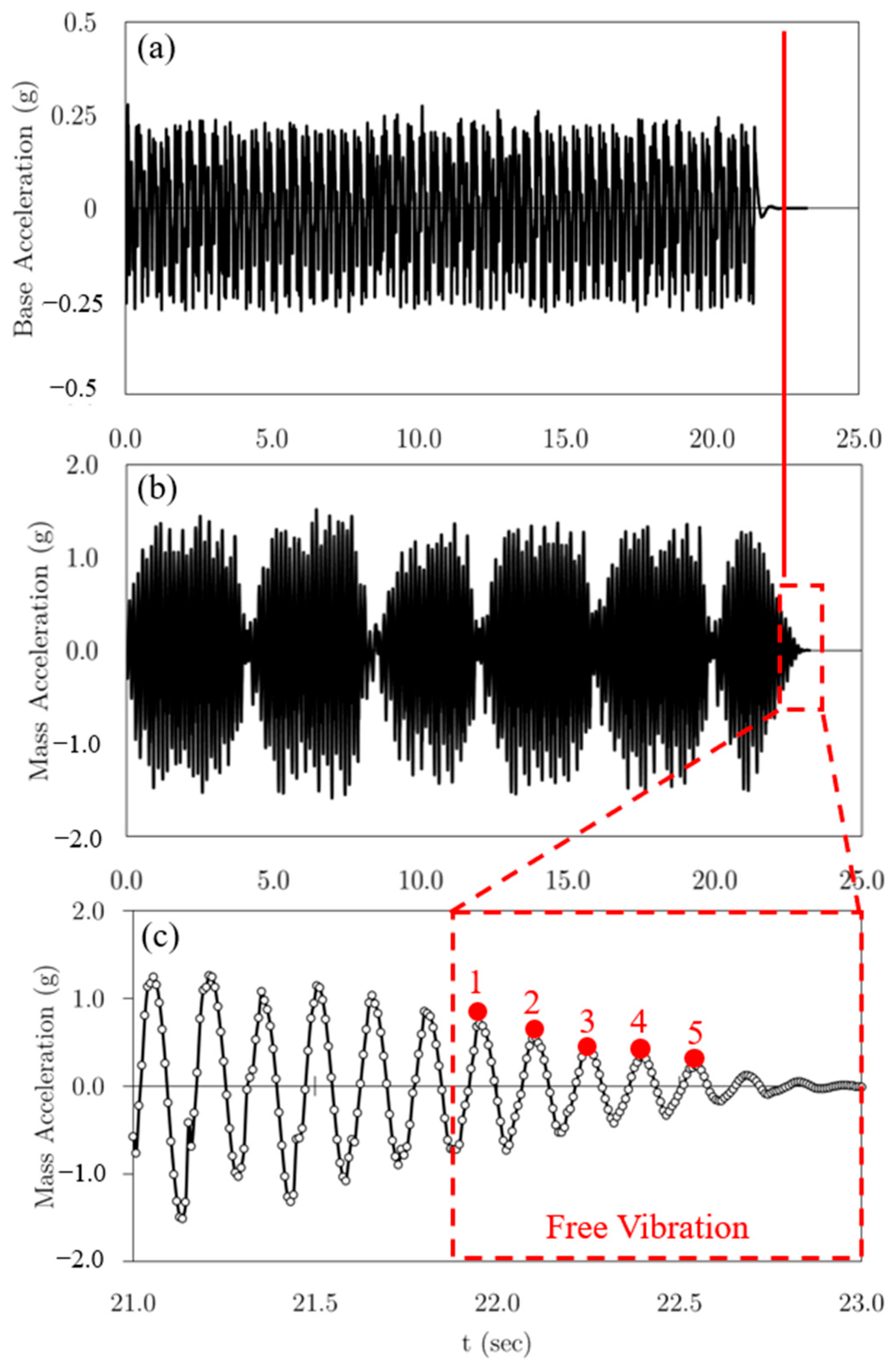
5.1. Laboratory Testing

Figure 10 shows the lab-bench setup established in a laboratory environment for testing the proof-of-concept prototype of EMEH under harmonic excitations. The apparatuses used in this experiment are a linear servo actuator (Dyadic Systems, SCN5-010-100, AS03) used as a shaker to simulate the harmonic excitation of base, a data logger system (WaveBook 516: Data Acquisition System) to record the output voltage, an acceleration sensor (Accelerometer Data Logger X2-5) to measure the acceleration of the base at a sampling rate of 125 Hz, and a PC to processes the output signals.

The center of the base plate was firmly attached to the shaker to drive the prototype EMEH by programmed harmonic excitations. The data logger was set to measure the time history of voltage at a sampling rate of 1000 Hz. The sensitivity and sampling rate of the accelerometer were set to 64,000 LSB/g and 125 Hz, respectively. The maximum acceleration of the harmonic excitation generated by the shaker was set to ü_bXmax = 0.2 g.

Figure 11 shows the power spectral density of the base acceleration for five different motion signals recorded by the accelerometer. These acceleration signals were denoised by a third-order band-pass Butterworth filter with the cut-off frequencies 0.5 Hz and 35 Hz and a Nyquist frequency of 62.5 Hz defined by the function [b,a] = butter(.) in MATLAB. This figure shows that the range of frequency of the base excitation is from f_b = 1.5 Hz to f_b = 3.0 Hz. This range is quite short, and the frequencies in this range are less than f_s = 6.5 Hz. This was due to the limitation of the actuator in compensating the gravity effects in the vertical direction (i.e., weight of the prototype EMEH). For this reason, exciting the prototype EMEH under a resonant condition when f_b = f_s = 6.5 Hz was not feasible in this experimental study.

Figure 12 shows the five voltage signals output from the prototype EMEH when subjected to the five base excitations with PSDs shown in Figure 11 for no load in the circuit (R_l ≅ 0). These voltage signals were denoised by a third-order band-pass Butterworth filter with the cut-off frequencies 3 Hz and 21 Hz and a Nyquist frequency of 500 Hz defined by function [b,a] = butter(.) in MATLAB.

The root mean squares (RMSs) of these voltage signals are 0.54 mV, 0.93 mV, 2.9 mV, 1.6 mV, and 1.3 mV, respectively. It should be noted a much higher voltage can be harvested from the device if one uses the PMs Array 2 in Figure 3.

5.2. Model Validation

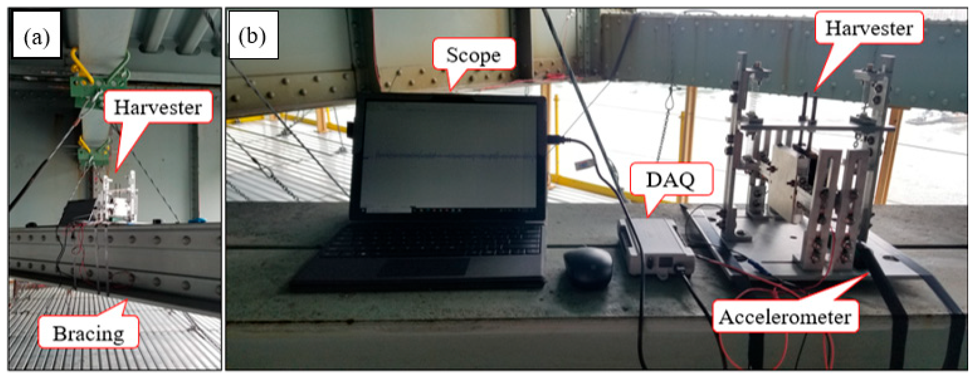
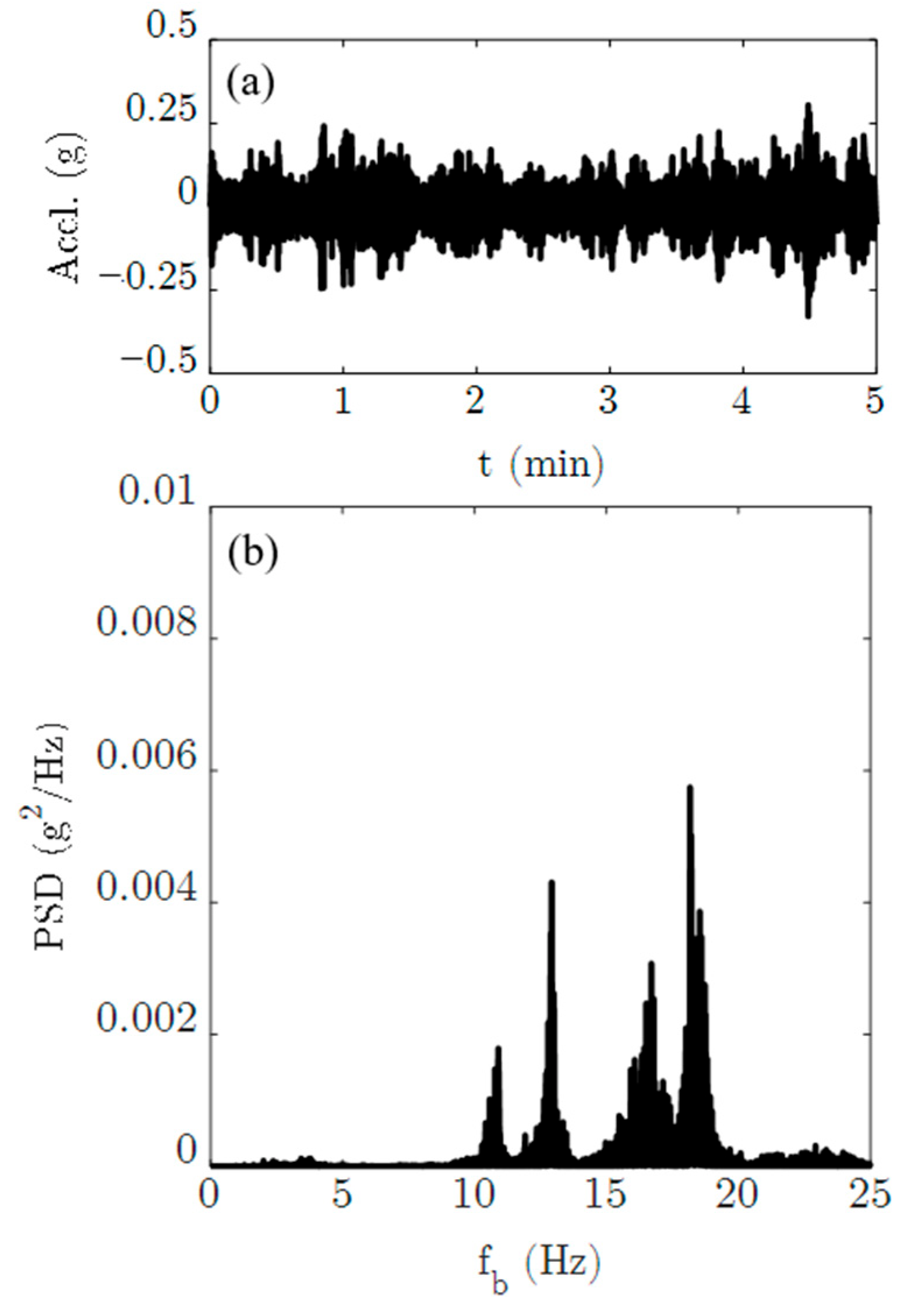
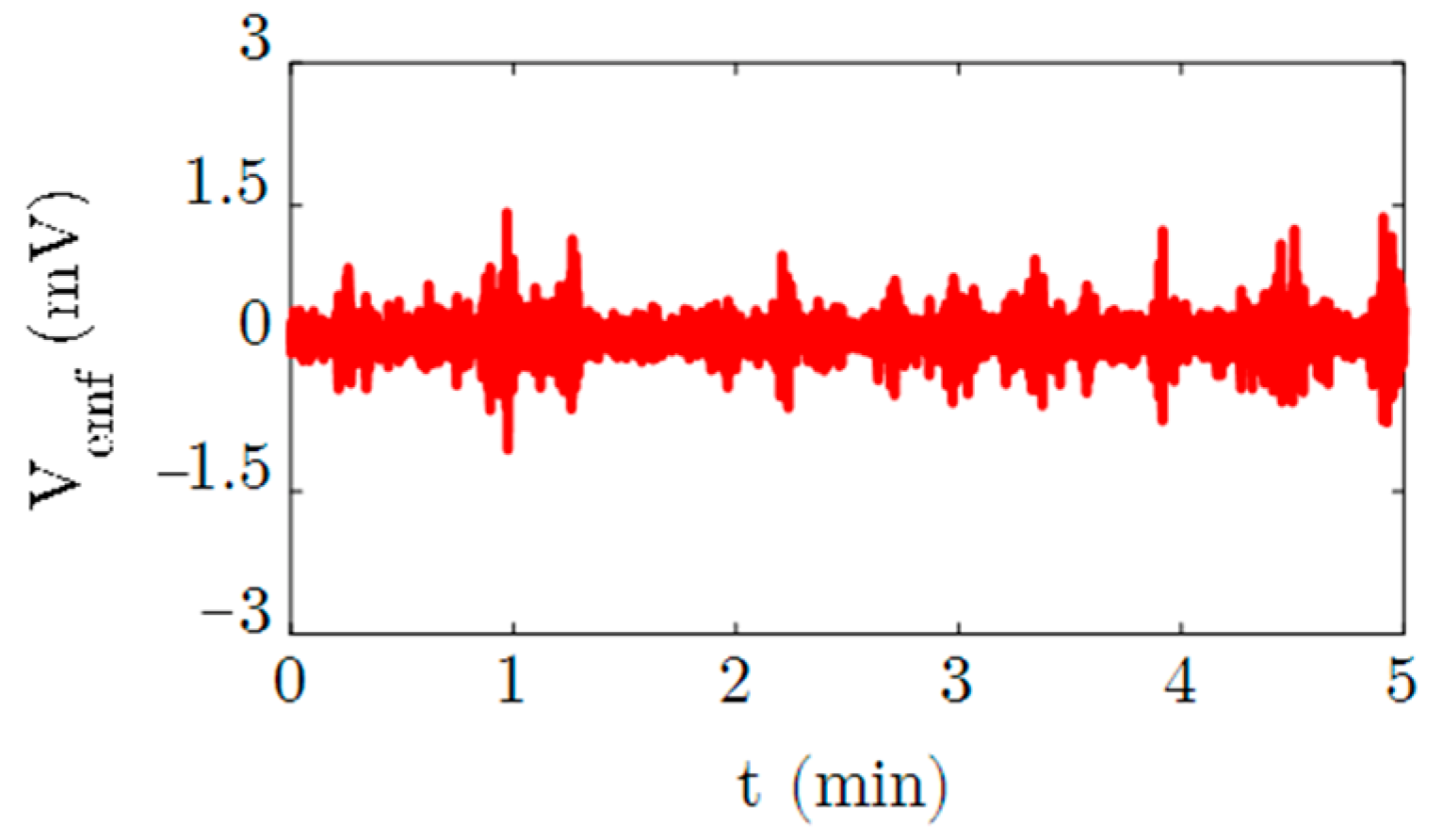
The accuracy of the proposed analytical model in predicting the eddy current damping force was verified in Section 3.2. This model is further validated by comparing the results of the analytical model to those obtained from the experimental model illustrated in Figure 10. Both the models are subjected to base acceleration No. 3 with the frequency f_b = 2.3 Hz as shown in Figure 11c. The parameters of the SDOF system are m_s = 0.49 kg, f_s = 6.5 Hz, and ξ_s. The mechanical damping ratio ξ_s is given by

$${\mathsf{\xi }}_{\mathrm{s}}={\mathsf{\xi }}_{\mathrm{t}}-\frac{{\mathrm{K}}_{\mathrm{f}}^2}{2{\mathrm{m}}_{\mathrm{s}}{\mathsf{\omega }}_{\mathrm{s}}\left({\mathrm{R}}_{\mathrm{l}}+{\mathrm{R}}_{\mathrm{c}}\right)}$$

(15)

in which the second term represents the electrical damping ratio which is estimated to be 0.1% by calculating ${\mathrm{K}}_{\mathrm{f}}\cong {\mathrm{N}}_{\mathrm{z}}{\mathrm{B}}_{\mathrm{mtavg}}\left({\mathrm{a}}_{\mathrm{c}}-{\mathrm{t}}_{\mathrm{c}}\right)=0.1 \mathrm{N}/\mathrm{A}$ for N_z = 6, ${\mathrm{B}}_{\mathrm{mtavg}}\cong 0.3 \mathrm{T}$ and ${\mathrm{a}}_{\mathrm{c}}-{\mathrm{t}}_{\mathrm{c}}=0.0508 \mathrm{m}$ and assuming that ${\mathrm{R}}_{\mathrm{l}}\cong 0.01{\mathrm{R}}_{\mathrm{c}}$ (no load) and the air gap is very small. The total damping ratio ${\mathsf{\xi }}_{\mathrm{t}}$ can be estimated from the free vibration response of tip mass by using the logarithmic decrement method as illustrated in Figure 13. This figure shows the time history of acceleration of the SDOF system recorded during the lab test. The average total damping is estimated to be 4.3%, implying that the mechanical damping ratio should be equal to ξ_s = 4.3−0.1 = 4.2%.

Therefore, the parameters of the SDOF system used in the simulation are: m_s = 0.49 kg, ξ_s = 4.2, and f_s = 6.5 Hz.

Table 4. Estimating the total damping ratio and frequency of SDOF system from free vibration results.

i	1	2	3	4	5
${\left[{\ddot{\mathrm{u}}}_{\mathrm{sX}}+{\ddot{\mathrm{u}}}_{\mathrm{bX}}\right]}_{\mathrm{i}} \left(\mathrm{g}\right)$	0.7090	0.5610	0.4160	0.3410	0.2410
${\mathrm{t}}_{\mathrm{i}}$ (sec)	22.952	22.248	22.400	22.544	22.688
Estimated Parameters
${\mathsf{\xi }}_{\mathrm{t}}$ (%)	3.7	4.8	3.1	5.5
${\mathrm{f}}_{\mathrm{s}}$ (Hz)	6.6	6.9	6.6	6.9

shows the estimated value of natural frequency of the SDOF system for five successive peaks. The average value of the natural frequency is about 6.75 Hz, which is very close to the 6.5 Hz used in the analytical model.

Figure 14 shows the voltage signal output from the prototype EMEH when subjected to the base excitation with f_b = 2.3 Hz (See Figure 11c). The RMS of this voltage signal is about 2.6 mV, which is close to 2.9 mV calculated from the recorded data for the corresponding base excitation.

5.3. Field Testing

A steel-girder bridge in New York City was selected for the field testing of the proof-of-concept prototype. The bridge is subjected to a quite strong vibration induced by a heavy daily traffic loading. The energy harvester was installed on one of the lateral horizontal bracings of the deck of the bridge at a location next to the end support as shown in Figure 15.

Figure 16a shows the time history of the acceleration of the bridge recorded by an accelerometer of the model Data Logger X2-5 over a time duration of 5 min. Figure 16b shows the power spectral density of the acceleration signal. It is seen that the bridge has several significant frequencies in a range from f_b = 10 Hz to f_b = 20 Hz. These frequencies are much larger than the frequency of the prototype which is about f_s = 4 Hz. For this reason, it was difficult to put the prototype EMEH into a resonant condition with the vibration of the bridge. Figure 17 shows the time history of the voltage output from the prototype EMEH during the field test. It is seen that the magnitude of this voltage is less than 1.5 mV.

6. Conclusions

This paper proposes an analytical method to study the application of planar magnetic arrays in the design of electromagnetic energy harvesters (EMEHs) that are used to harvest electrical power from the vibrations of highway bridges. The proposed analytical method is capable of accurately describing the electromechanical coupling between the electrical and mechanical domains. Three steps are taken to formulize the generation of electrical power in this method: (1) calculating the magnetic flux density vector of permanent magnets (PMs) arranged in special arrays by solving the magnetostatic form of Maxwell’s equations, (2) calculating the magnetic flux density vector of coil by using the shell method, and (3) calculating the magnetic force acting on the coil by using the integral form of Lorentz force in electromagnetism. The force formula in step 3 is used to calculate the variation of the electromechanical coupling coefficient with respect to time. This is an important result of this paper, as in many previous research works this coefficient has been assumed to be constant. This is an over-simplified assumption that results in errors when calculating the electrical power. The accuracy of the proposed analytical method has been verified by developing a 3D finite element (FE) model of a simple EMEH in COMSOL. This analytical method is used to design an electromagnetic energy harvester in which planar arrays of PMs have been employed as the magnetic field source to interact with the moving copper coil. A parametric analysis was carried out on the arrangements of PMs and the electrical resistance of the harvesting circuit under a resonance condition. The analysis was performed for seven different multipole arrays including: (1) uniform, (2) X-linear alternating, (3) Y-linear alternating, (4) planar alternating, (5) X-linear Halbach, (6) Y-linear Halbach, and (7) planar Halbach arrays. It was found that the EMEH can deliver the highest electrical power when the PMs are arranged according to Array 2, in which the poles alternate along the direction of motion. The numerical results showed that, for ü_bXmax = 0.1 g, the maximum average electrical power is equal to 513 mW that can be delivered by a harvesting circuit with an electrical resistance of 186.6 mΩ. Furthermore, a proof-of-the-concept prototype was fabricated for the laboratory and field testing in which Array 4 was selected to arrange the PMs poles. The laboratory testing showed that the RMSs of voltage outputted from the harvester when subjected to a base excitation with a frequency ranging from f_b = 1.5 Hz to f_b = 3.0 Hz (below the resonant frequency of the harvester) varies from 0.54 mV to 2.9 mV. The field testing of the harvester also showed that the harvester can generate a voltage as large as 1.5 mV for an excitation frequency in the range of 10 Hz to 20 Hz. The experimental study carried out in this paper was limited to one type of planar magnetic array (planar alternating) without considering the resonant condition. A more comprehensive experimental study of such electromagnetic harvesters with planar magnetic array will be the subject of future publication of the authors.

References

1. Roundy, S.; Wright, P.K.; Rabaey, J.M. Energy Scavenging for Wireless Sensor Networks; Springer: New York, NY, USA, 2004. [Google Scholar]
2. Williams, C.; Yates, R. Analysis of a micro-electric generator for microsystems. Sens. Actuators A Phys. 1996, 52, 8–11. [Google Scholar] [CrossRef]
3. Stosiak, M. The impact of hydraulic systems on the human being and the environment. J. Theor. Appl. Mech. 2015, 53, 409–420. [Google Scholar] [CrossRef] [Green Version]
4. Priya, S.; Inman, D.J. (Eds.) Energy Harvesting Technologies; Springer: New York, NY, USA, 2009; pp. 337–350. ISBN 9780387764634. [Google Scholar]
5. Amjadian, M.; Agrawal, A.K. Planar arrangement of permanent magnets in design of a magneto-solid damper by finite element method. J. Intell. Mater. Syst. Struct. 2020, 31, 998–1014. [Google Scholar] [CrossRef]
6. Amjadian, M.; Agrawal, A.K. A passive electromagnetic eddy current friction damper (PEMECFD): Theoretical and analytical modeling. Struct. Control Health Monit. 2017, 24, e1978. [Google Scholar] [CrossRef]
7. Amjadian, M.; Agrawal, A.K. Modeling, design, and testing of a proof-of-concept prototype damper with friction and eddy current damping effects. J. Sound Vib. 2018, 413, 225–249. [Google Scholar] [CrossRef]
8. Sazonov, E.; Li, H.; Curry, D.; Pillay, P. Self-Powered Sensors for Monitoring of Highway Bridges. IEEE Sens. J. 2009, 9, 1422–1429. [Google Scholar] [CrossRef] [Green Version]
9. Kwon, S.-D.; Park, J.; Law, K. Electromagnetic energy harvester with repulsively stacked multilayer magnets for low frequency vibrations. Smart Mater. Struct. 2013, 22, 055007. [Google Scholar] [CrossRef] [Green Version]
10. Green, P.L.; Papatheou, E.; Sims, N.D. Energy harvesting from human motion and bridge vibrations: An evaluation of current nonlinear energy harvesting solutions. J. Intell. Mater. Syst. Struct. 2013, 24, 1494–1505. [Google Scholar] [CrossRef] [Green Version]
11. Pirisi, A.; Mussetta, M.; Grimaccia, F.; Zich, R.E. Novel Speed-Bump Design and Optimization for Energy Harvesting from Traffic. IEEE Trans. Intell. Transp. Syst. 2013, 14, 1983–1991. [Google Scholar] [CrossRef]
12. Gatti, G.; Brennan, M.J.; Tehrani, M.G.; Thompson, D.J. Harvesting energy from the vibration of a passing train using a single-degree-of-freedom oscillator. Mech. Syst. Signal Process. 2016, 66–67, 785–792. [Google Scholar] [CrossRef] [Green Version]
13. Takeya, K.; Sasaki, E.; Kobayashi, Y. Design and parametric study on energy harvesting from bridge vibration using tuned dual-mass damper systems. J. Sound Vib. 2016, 361, 50–65. [Google Scholar] [CrossRef]
14. Ahmad, M.M.; Khan, F.U. Dual Resonator-Type Electromagnetic Energy Harvester for Structural Health Monitoring of Bridges. J. Bridg. Eng. 2021, 26, 04021021. [Google Scholar] [CrossRef]
15. Amjadian, M.; Agrawal, A.K.; Nassif, H. Feasibility of using a high-power electromagnetic energy harvester to power structural health monitoring sensors and systems in transportation infrastructures. Proc. SPIE 2021, 2021, 115911G. [Google Scholar] [CrossRef]
16. Peigney, M.; Siegert, D. Low-Frequency Electromagnetic Energy Harvesting from Highway Bridge Vibrations. J. Bridg. Eng. 2020, 25, 04020056. [Google Scholar] [CrossRef]
17. El-Hami, M.; Glynne-Jones, P.; White, N.; Hill, M.; Beeby, S.; James, E.; Brown, A.; Ross, J. Design and fabrication of a new vibration-based electromechanical power generator. Sens. Actuators A Phys. 2001, 92, 335–342. [Google Scholar] [CrossRef]
18. Beeby, S.P.; Torah, R.N.; Tudor, M.J.; Glynne-Jones, P.; O’Donnell, T.; Saha, C.R.; Roy, S. A micro electromagnetic generator for vibration energy harvesting. J. Micromech. Microeng. 2007, 17, 1257–1265. [Google Scholar] [CrossRef]
19. Zeng, P.; Khaligh, A. A Permanent-Magnet Linear Motion Driven Kinetic Energy Harvester. IEEE Trans. Ind. Electron. 2013, 60, 5737–5746. [Google Scholar] [CrossRef]
20. Elvin, N.G.; Elvin, A.A. An Experimentally Validated Electromagnetic Energy Harvester. J. Sound Vib. 2011, 330, 2314–2324. [Google Scholar] [CrossRef]
21. Halim, M.A.; Cho, H.; Park, J.Y. Design and experiment of a human-limb driven, frequency up-converted electromagnetic energy harvester. Energy Convers. Manag. 2015, 106, 393–404. [Google Scholar] [CrossRef]
22. Salauddin, M.; Halim, M.A.; Park, J.Y. A magnetic-spring-based, low-frequency-vibration energy harvester comprising a dual Halbach array. Smart Mater. Struct. 2016, 25, 095017. [Google Scholar] [CrossRef]
23. Liu, X.; Qiu, J.; Chen, H.; Xu, X.; Wen, Y.; Li, P. Design and Optimization of an Electromagnetic Vibration Energy Harvester Using Dual Halbach Arrays. IEEE Trans. Magn. 2015, 51, 8204204. [Google Scholar] [CrossRef]
24. Yang, B.; Lee, C.; Xiang, W.; Xie, J.; He, J.H.; Kotlanka, R.K.; Low, S.P.; Feng, H. Electromagnetic energy harvesting from vibrations of multiple frequencies. J. Micromech. Microeng. 2009, 19, 035001. [Google Scholar] [CrossRef]
25. Foisal, A.R.M.; Hong, C.; Chung, G.-S. Multi-frequency electromagnetic energy harvester using a magnetic spring cantilever. Sens. Actuators A Phys. 2012, 182, 106–113. [Google Scholar] [CrossRef]
26. Mikoshiba, K.; Manimala, J.M.; Sun, C.T. Energy harvesting using an array of multifunctional resonators. J. Intell. Mater. Syst. Struct. 2013, 24, 168–179. [Google Scholar] [CrossRef]
27. Soliman, M.S.M.; Abdel-Rahman, E.; El-Saadany, E.F.; Mansour, R.R. A wideband vibration-based energy harvester. J. Micromech. Microeng. 2008, 18, 115021. [Google Scholar] [CrossRef]
28. Arroyo, E.; Badel, A.; Formosa, F.; Wu, Y.; Qiu, J. Comparison of electromagnetic and piezoelectric vibration energy harvesters: Model and experiments. Sens. Actuators A Phys. 2012, 183, 148–156. [Google Scholar] [CrossRef]
29. Zhu, D.; Beeby, S.; Tudor, J.; Harris, N. Vibration energy harvesting using the Halbach array. Smart Mater. Struct. 2012, 21, 075020. [Google Scholar] [CrossRef]
30. Salauddin, M.; Park, J.Y. Design and experiment of human hand motion driven electromagnetic energy harvester using dual Halbach magnet array. Smart Mater. Struct. 2017, 26, 035011. [Google Scholar] [CrossRef]
31. Zhu, D.; Beeby, S.; Tudor, J.; Harris, N. Increasing output power of electromagnetic vibration energy harvesters using improved Halbach arrays. Sens. Actuators A Phys. 2013, 203, 11–19. [Google Scholar] [CrossRef] [Green Version]
32. Furlani, E.P. Permanent Magnet and Electromechanical Devices; Academic Press: Cambridge, MA, USA, 2001; ISBN 0122699513. [Google Scholar]
33. Robertson, W.; Cazzolato, B.; Zander, A. Axial Force Between a Thick Coil and a Cylindrical Permanent Magnet: Optimizing the Geometry of an Electromagnetic Actuator. IEEE Trans. Magn. 2012, 48, 2479–2487. [Google Scholar] [CrossRef]
34. Paul, C.R. Inductance; John Wiley & Sons, Inc.: Hoboken, NJ, USA, 2009; ISBN 9780470561232. [Google Scholar]
35. Cannarella, J.; Selvaggi, J.; Salon, S.; Tichy, J.; Borca-Tasciuc, D.-A. Coupling Factor Between the Magnetic and Mechanical Energy Domains in Electromagnetic Power Harvesting Applications. IEEE Trans. Magn. 2011, 47, 2076–2080. [Google Scholar] [CrossRef]
36. Mösch, M.; Fischerauer, G. A Comparison of Methods to Measure the Coupling Coefficient of Electromagnetic Vibration Energy Harvesters. Micromachines 2019, 10, 826. [Google Scholar] [CrossRef] [PubMed] [Green Version]
37. Multiphysics® Modeling Software, Version 5.4; COMSOL: Burlington, MA, USA, 2018.
38. Sams, H.W. Handbook of Electronics Tables and Formulas; Howard W. Sams & Co.: Carmel, IN, USA, 1986; ISBN 0672224690. [Google Scholar]
39. Amjadian, M.; Agrawal, A.K. Feasibility study of using a semiactive electromagnetic friction damper for seismic response control of horizontally curved bridges. Struct. Control Health Monit. 2019, 26, e2333. [Google Scholar] [CrossRef]
40. MATLAB, Version R2017b; The MathWorks Inc.: Natick, MA, USA, 2017.
41. Stephen, N. On energy harvesting from ambient vibration. J. Sound Vib. 2006, 293, 409–425. [Google Scholar] [CrossRef] [Green Version]
42. Zhu, S.; Shen, W.-A.; Xu, Y.-L. Linear electromagnetic devices for vibration damping and energy harvesting: Modeling and testing. Eng. Struct. 2012, 34, 198–212. [Google Scholar] [CrossRef] [Green Version]
43. Zuo, L.; Cui, W. Dual-Functional Energy-Harvesting and Vibration Control: Electromagnetic Resonant Shunt Series Tuned Mass Dampers. J. Vib. Acoust. 2013, 135, 051018. [Google Scholar] [CrossRef] [Green Version]
44. Shen, W.; Zhu, S.; Xu, Y.-L.; Zhu, H.-P. Energy regenerative tuned mass dampers in high-rise buildings. Struct. Control Health Monit. 2018, 25, e2072. [Google Scholar] [CrossRef]
Figure 1. Configuration of the EMEH and its key components. (a) Vertical cross section of the EMEH in the XZ-plane. (b) Geometrical parameters of the arrays in details.
Energies 15 03540 g001
Figure 2. Electromechanical model of the EMEH consisting of a lumped SDOF dynamic system coupled to a lumped first-order RL circuit.
Energies 15 03540 g002
Figure 3. Planar arrangement of the PMs poles in seven different multipole arrays with their corresponding parameters: (a) uniform, (b) X-linear alternating, (c) Y-linear alternating, (d) planar alternating on the left and right sides; and the top faces of (e) X-linear Halbach, (f) Y-linear Halbach, (g) planar Halbach arrays on the right sides, and the top faces of (h) X-linear Halbach, (i) Y-linear Halbach, and (j) planar Halbach arrays on the left side.
Energies 15 03540 g003
Figure 4. Geometrical parameters of the coil in details; (a) cross-section in the xy-plane; (b) cross-section in the xz-plane; and (c) the equivalent PM of p-turn.
Energies 15 03540 g004
Figure 5. FE model used for validation of the force-current model developed in this study: (a) longitudinal cross section on the XZ-Plane, (b) XY-Plane, (c) FE model enclosed by the air domain; and (d) Bmt-field on the XZ-plane at Y = 0 for usX = −0.216ac and Ici = −0.849 A.
Energies 15 03540 g005
Figure 6. Comparison between the analytical model and the FE model to calculate the magnetic force; (a) displacement of the coil, (b) electric current induced in the coil, and (c) magnetic force acting on the coil.
Energies 15 03540 g006
Figure 7. Variation of the electromechanical coupling coefficient with (a) time and (b) displacement of the coil.
Energies 15 03540 g007
Figure 8. Average electrical power harvested from the EMEH versus the ratio of the load resistance to the coil resistance (Rl/Rc) for (a) Array 1, (b) Array 2, (c) Array 3, (d) Array 4, (e) Array 5, (f) Array 6, and (g) Array 7.
Energies 15 03540 g008
Figure 9. Proof-of-concept prototype of the EMEH; (a) 3D view of the fabricated device in laboratory with details of the geometry of (b,c) the arrays and (d) the copper coil.
Energies 15 03540 g009
Figure 10. Experimental setup established to test the proof-of-concept prototype of EMEH in a laboratory environment under harmonic excitations.
Energies 15 03540 g010
Figure 11. Power spectral density of the acceleration of base recorded by an accelerometer of the model Data Logger X2-5.
Energies 15 03540 g011
Figure 12. Voltage output from the prototype EMEH subjected to five different base excitations with the frequencies from fb = 1.5 Hz to fb = 3.0 Hz; RMSs of these voltage signals are (a) 0.54 mV, (b) 0.93 mV, (c) 2.9 mV, (d) 1.6 mV, and (e) 1.3 mV.
Energies 15 03540 g012
Figure 13. Time history responses of the SDOF system recorded during the lab testing; (a) base acceleration fb = 2.3 Hz, (b) tip mass acceleration (proper), and (c) tip mass acceleration under a free vibration.
Energies 15 03540 g013
Figure 14. Voltage output from the SDOF model subjected to base excitations with the frequency from fb = 2.3 Hz.
Energies 15 03540 g014
Figure 15. Field testing of the proof-of-concept prototype of EMEH (a) placement of the device on the middle of a horizontal lateral bracing of the deck, and (b) testing setup.
Energies 15 03540 g015
Figure 16. Acceleration of the base excitation recorded by an accelerometer of the model Data Logger X2-5 during the field testing: (a) 5 min time-history of the acceleration and (b) power spectral density of the acceleration.
Energies 15 03540 g016
Figure 17. Voltage output from the prototype EMEH subjected to vibration of the bridge.
Energies 15 03540 g017