Energy-Saving Potential of Thermal Diode Tank Assisted Refrigeration and Air-Conditioning Systems

Abstract

Lowering the condensing temperature of the Refrigeration and Air-conditioning (RAC) system has been proven to effectively increase the system’s Coefficient of Performance (COP). This paper revolves around evaluating the energy-saving generated by applying a Thermal Diode Tank (TDT) in the RAC systems. The TDT is a novel invention, which is an insulated water tank equipped with gravity heat pipes. If the TDT was placed outdoors overnight, its inside water would theoretically be at the minimum ambient temperature of the previous night. When the TDT water is used to cool the condenser of RAC systems that operate during the daytime, a higher COP of this TDT assisted RAC (TDT-RAC) system could be achieved compared with the baseline system. In this study, a steady-state performance simulation model for TDT-RAC cycles has been developed. The model reveals that the COP of the TDT-RAC cycle can be improved by 10~59% over the baseline cycle depending on the compressor types. The TDT-RAC cycle with a variable speed compressor can save more energy than that with a fixed speed compressor. In addition, TDT-RAC cycles can save more energy with a higher day/night ambient temperature difference. There is a threshold tank size for a given TDT-RAC cycle to save energy, and the energy-saving can be improved by enlarging the tank size. A desk-top case study based on real weather data for Adelaide in January 2021 shows that 9~40% energy could be saved by TDT-RAC systems every summer day on average.

1. Introduction

Conserving energy is a major global challenge, and one of the most effective methods is to find solutions from energy efficiency improvements. Due to the rapid development of the world economy, ever more public buildings have been built, leading to an increasing requirement of heating, ventilation, and air-conditioning (HVAC) [1]. According to the projections of Australian Government′s Department of Climate Change and Energy Efficiency in 2012 [2], electricity is the main source of energy for commercial buildings, accounting for about 50% of the above-mentioned total energy consumption, of which HVAC are usually the largest end-users of electricity. In addition, about 20~30% of energy consumption is yielded by the refrigeration and air-conditioning (RAC) system, producing over 34.7 Mt of total carbon emissions [3].

The report ‘State of the Climate 2020: Bureau of Meteorology’ [4] predicted that Australia is facing a trend of continued climate warming. Australia straddles a mainly temperate climate in densely populated coastal areas, which is characterised by large day and night ambient temperature differences in summer [5]. Since the average annual temperature in Australia is relatively high, and the hot period is much longer than the cold period, the demand for cooling is much greater than for heating. Moreover, traditional cooling demand industries such as food and pharmaceutical factories, datacentres, and wine industries, all make growing demands for more refrigeration and air-conditioning [1]. Consequently, improving the energy efficiency of cooling systems has greater significance than improving heating systems.

Lowering the condensing temperature of the RAC system has been validated to effectively increase the system’s Coefficient of Performance (COP). Walsh [6] found that the COP for a RAC system normally ranges from 0 to 7 if no condenser cooling measures are applied. A 1 °C decrease in the condensing temperature would result in a 3.23% augmentation in the COP [7]. One of the successful examples of condenser cooling measure is the application of Ground-sourced RAC (GSRAC) systems, as the average underground soil temperature is lower than the ambient temperature during the day time in summer. A typical GSRAC system can reduce 30~40% energy compared with a normal RAC system (baseline system). However, GSRAC system would occupy considerable land resources to drill and install boreholes, which could be up to 200 m deep, and their payback periods are too long, basically over 7 years [8,9,10].

In addition to GSRAC systems, many other measures have been developed to lower the condensing temperature and improve the COP of the RAC system. Zhang et al. [11] examined an integrated RAC system with evaporative air-coolers that cool the air before it enters the condenser. The COP of this integrated system shows a 39% increase in the COP under the hot-arid area of China. Wang et al. [12] also utilised an evaporative cooling condenser in an existing air-conditioning system, which yielded a COP augmentation by 12%. Another experiment conducted by Yu and Chan [13] found that the evaporative coolers could increase the COP of air-cooled chillers by up to 20%. However, the energy-saving performance of these evaporative coolers would be reduced with the higher humidity, so their applications in most humid regions are limited. Waly et al. [14] also experimented with an evaporative cooling method, in which the inlet air was cooled by the spraying water before entering the condenser, and their results indicated an increase in COP by 36%. In this experiment, a problem was faced that the condenser should be placed away from obstructions because the shading of condenser would reduce the COP.

Chen et al. [15] assessed the ability of liquid–vapor separation condensers (LSC) and found that the COP of the LSC system was improved by 11.1% compared with the baseline system. To further improve the LSC system, Zhong et al. [16] studied the impact of a double-row liquid–vapor separation condenser (DLSC) on the RAC system cooling performance. This novel condenser achieved an improvement in the COP by about 30%. In both researches, the cooling performance of separation condensers is constrained by the ambient temperature; if the ambient temperature was over 40 °C, these systems would even have lower COPs.

While utilising the mist generator to supply cold mist for the RAC system’s condenser, Yang et al. [17] achieved a considerable COP improvement of 21.3~51.5%, which is higher than those of most evaporative cooling methods. In application, the mist generator requires an open-loop water tower that consumes water to produce mist, which would be a waste of water resource.

Above literatures revealed that the performance enhancement of RAC systems was achieved using different condenser cooling methods, with significant COP improvements. However, there is little investigation on how to calculate the theoretical value of COP in vapor compression refrigeration cycles when the condenser cooling methods are applied. In addition to the defects and deficiencies summarized above, extra energy is also required to run the cooling units, such as air-coolers and mist generators.

In this paper, the Thermal Diode Tank (TDT) is a potential cost-effective alternative of other condenser cooling measures to supply water-cooling for RAC systems. Unlike above-mentioned studies, the TDT works automatically and passively that does not consume additional energy or resources. Basically, a TDT is an insulated water tank equipped with gravity heat pipes, which can passively release heat to the ambient air if the ambient temperature is lower than the water temperature inside TDT, but would not allow the heat to enter the tank even when the ambient temperature is higher. The RAC system equipped with a TDT is expected to generate a reduction of up to 40% in its energy consumption compared with a baseline system in the presence of day and night ambient temperature differences. However, since TDT is a newly invented technology, there has been little systematic research into it. Correlations between the design and operation parameters of TDT and its improvement are unknown. The aim of this study is to understand the potential of TDT when it is used to supply cooling water to a baseline system, by conducting desk-top case studies.

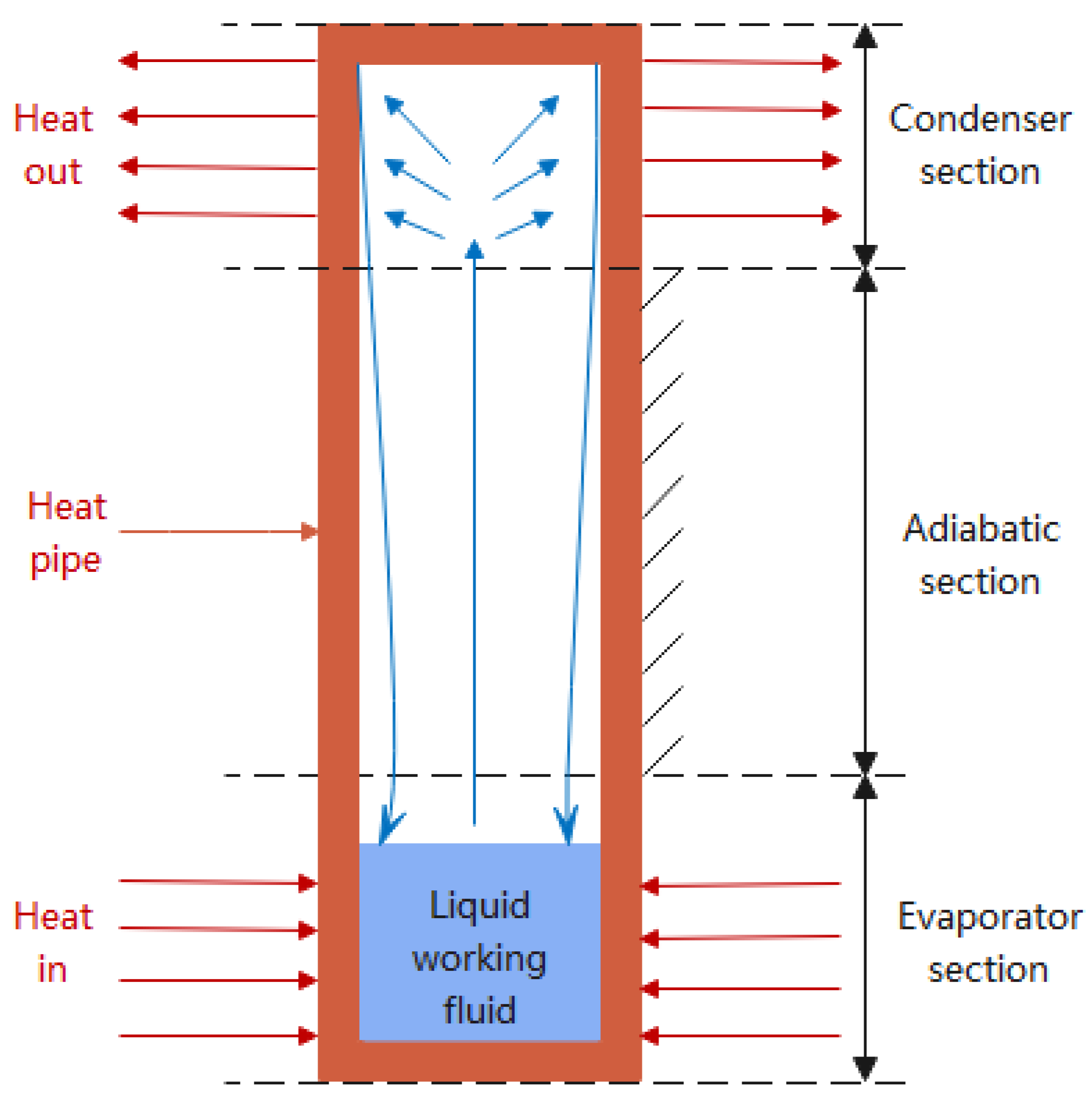
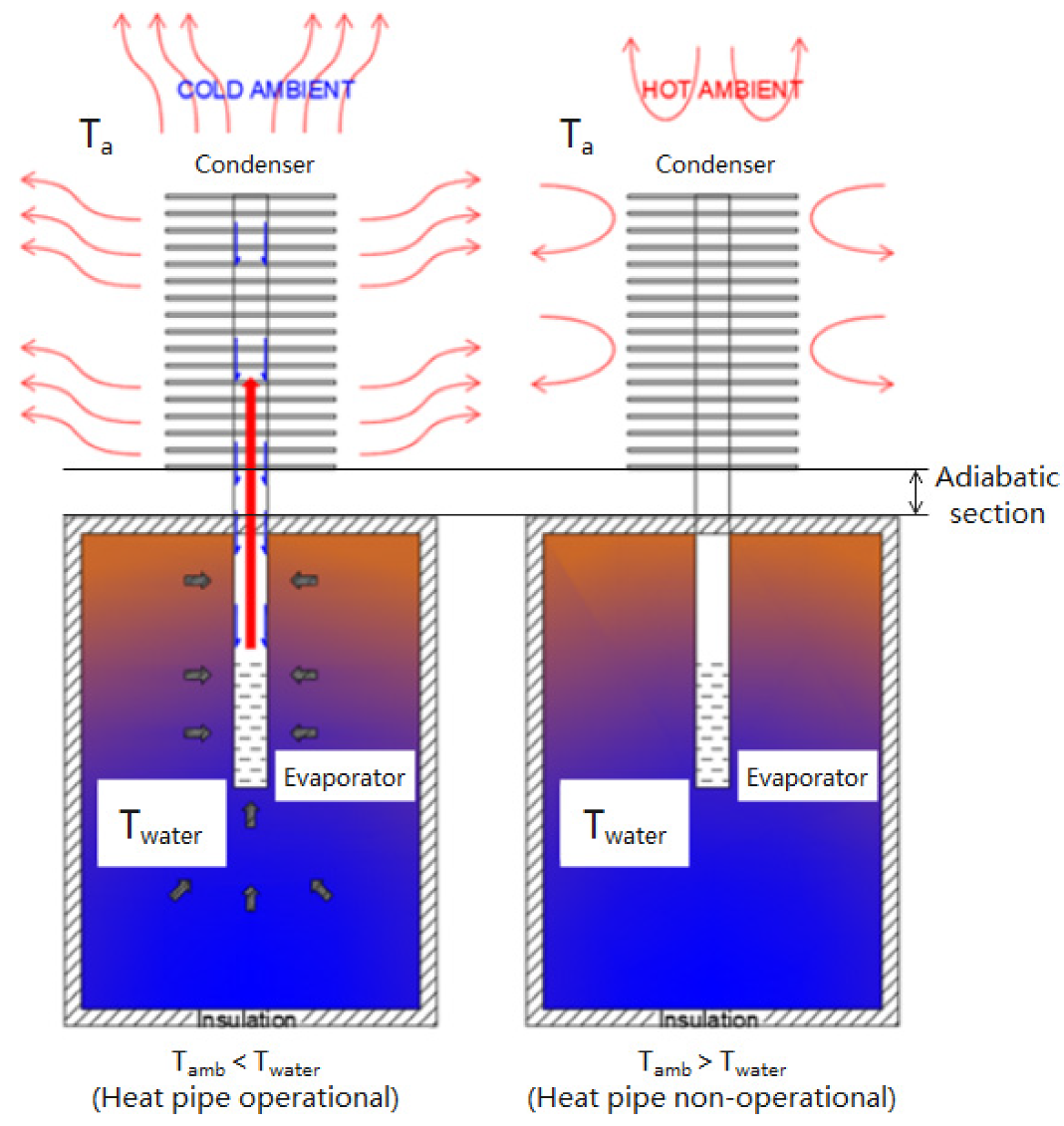
2. Thermal Diode Tank (TDT)

The TDT was proposed by Hu and Kimenkowski in 2019, which is constructed as a well-insulated water tank equipped with gravity heat pipes. The Gravity Heat Pipe (GHP, shown in Figure 1) is an isolated pipe containing a working fluid that coexists in liquid and vapor states [18]. When the temperature at the evaporator section of the GHP is higher, the working fluid (water, R134a, ammonia, etc.) will evaporate from liquid to vapor phase. The vapor rises upwards where the temperature is lower than that at the evaporator section, and condenses to release heat at the condenser section. After the vapor condenses, the condensate (liquid working fluid) flows back to the evaporator section due to the gravity [19]. A continuous circulation inside the GHP can be established if the evaporator temperature is higher than the condenser temperature. Oppositely, the heat will not be transferred downwards even though the condenser temperature is higher than the evaporator temperature. Therefore, the GHP functions as a thermal diode and automatically transfers heat only in one direction, from evaporator to condenser [20]. The thermal resistance inside a GHP is almost nil, so this device is very efficient in heat transfer. In practice, if the GHP evaporator temperature was higher than its condenser temperature by 1 °C or more, it would start operating.

The conceptual working diagram of the TDT is illustrated in Figure 2. With the one-direction heat transfer capability provided by GHPs, the TDT can release heat to the ambient air only if its inside water temperature is higher than the ambient temperature, but the heat from outside cannot enter the TDT. The adiabatic section of the GHPs prevents the heat from being transferred from the condenser section to the evaporator section by conduction even with scorching ambient temperatures. If such a device was placed outdoors overnight, the TDT water would theoretically be at the minimum ambient temperature of the last night. Thus, the TDT can passively harvest cold energy from the day/night ambient temperature differences to produce cooling water to lower the condensing temperature of the RAC system.

Figure 3 shows the schematic diagram of the proposed TDT-RAC system. When the water at the minimum ambient temperature of the previous night is used to cool the RAC system’s condenser, the COP of this integrated system would increase significantly. Namely, during the day time, the TDT-RAC system virtually works at a minimum ambient temperature of the last night. It is predicted that a lower night ambient temperature and a larger tank size are more beneficial to the TDT-RAC system, since colder and more cooling water can be produced for the RAC system’s condenser.

3. Modelling of TDT-RAC Cycles

To evaluate the energy-saving performance of TDT-RAC systems compared with the baseline system, steady-state performance simulation models for TDT-RAC cycles were developed.

3.1. Baseline Cycle

The cycle COP of a vapour compression RAC system in Figure 4 can be expressed in terms of enthalpies [21]:

$$CO{P}_{cycle 1}=\frac{{\dot{Q}}_{RAC}}{{\dot{W}}_C}=\frac{h_1-h_4 }{h_2-h_1 }$$

(1)

where

$${\dot{Q}}_{RAC}={\dot{m}}_1\left(h_1-h_4\right)$$

(2)

$${\dot{W}}_C={\dot{m}}_1\left(h_2-h_1\right)$$

(3)

and ${\dot{m}}_1$ (kg/s) is the refrigerant mass flow rate of the baseline cycle (Cycle 1), and h (kJ/kg) represents the specific enthalpy.

From Equation (1), it is observed that the COP can be improved theoretically by either increasing the enthalpy gap between h₁ and h₄, and/or decreasing the enthalpy gap between h₂ and h₁. It is noted that h₁ depends on the required evaporating temperature (T₁), which it is unable to vary, otherwise the cooling demand cannot be met. Therefore, in engineering practice, h₄ and/or h₂ are lowered to improve the COP of the RAC system. From state 3 to 4, the refrigerant passes the expansion valve where there is no energy transfer, so the enthalpy during this process is constant (h₃ = h₄). Therefore, h₄ and h₂ both depend on the condensing temperature (T₃), and an improvement in COP can be achieved by lowering the condensing temperature of the RAC system.

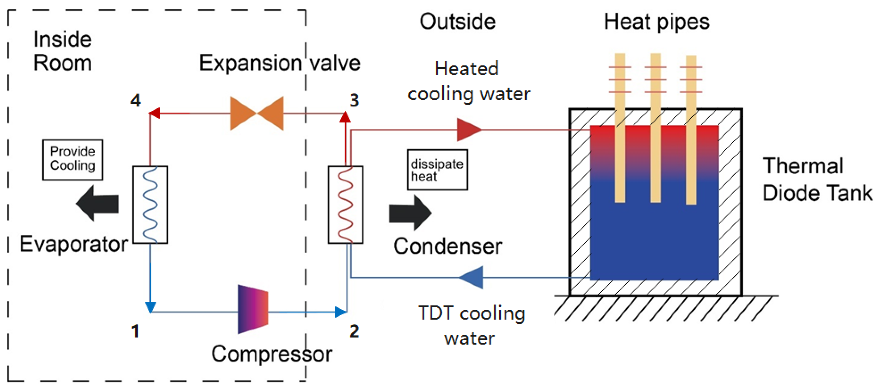
3.2. TDT-RAC Cycles

Depending on the compressor type (i.e., fixed speed or variable speed) of RAC systems, the impacts of the TDT on the RAC cycle are different. A fixed speed compressor always runs at a full capacity, while a variable speed compressor virtually runs at 25% to 100% capacity [22]. Figure 5 illustrates the differences in cycles in T-s diagrams with different compressors when the condensing temperature decreases. Figure 5a shows the TDT-RAC cycle with a fixed speed compressor (Cycle 2), in which the cycle 1→2→3→4→1 represents the baseline cycle, and Figure 5b shows the TDT-RAC cycle with a variable speed compressor (Cycle 3):

For the TDT-RAC Cycle 2 (1→2→3′→4′→1) in Figure 5a or Figure 6a, the refrigerant state at the condenser would be state 3′ (undercooled liquid) rather than state 3 (saturated liquid) because the condensing temperature (T_3′) is lowered by the TDT water, but the pressure at state 3′ is still equal to that at state 3. Hence, h_4′ is decreased from h₄, while the compressor work remains unaffected. Consequently, the refrigeration effect (h₁–h_4′) in the TDT-RAC cycle is greater than that in the baseline cycle, (h₁–h₄).

For Cycle 3 (1→2″→3″→4″→1) in Figure 5b or Figure 6b, the refrigerant state at the condenser would be state 3″ (saturated liquid) instead of state 3 due to the reduced condensing temperature (T_3″) generated by the TDT. The saturated refrigerant is cooled, causing a pressure drop, and h_4″ becomes smaller than h₄. Meanwhile, the variable speed compressor works at a lower speed to produce less heat, so that the refrigerant is cooled from state 2 to state 2″. Therefore, the refrigeration effect (h₁–h_4″) in the TDT-RAC cycle is greater than that in the normal RAC cycle (h₁–h₄), while the compressor work in the TDT-RAC cycle (h_2″–h₁) is lower than that in the normal RAC cycle (h₂–h₁).

3.3. Mathematical Model

The mathematical model developed in this study is a steady-state performance simulation model and its inputs and outputs are presented in

Table 1. Inputs and outputs of performance simulation (mathematical) model.

Inputs
${\dot{Q}}_{RAC}$	RAC system cooling capacity (kW)
$T_{room}$	Room temperature set (°C)
$T_a$	Day time ambient temperature (°C)
$T_{night}$	Minimum ambient temperature (last night) (°C)
$T_{water}$	TDT water temperature (early morning) (°C)
$\Delta t$	Time interval (hour)
$t_{RAC}$	Total operation time (hour)
$V$	Tank size (m3)
$C_P$	Specific heat capacity of water = 4.18 (kJ/kg °C)
$\rho$	Density of TDT water = 1000 (kg/m3)
Outputs
COP	COP for each time interval
COPaverage	Average COP over tRAC

. Following assumptions are made in the model:

• The TDT is well insulated and has heat transfer with surroundings only through heat pipes;
• The temperature of water inside TDT is uniform at any times;
• The process from 1 to 2 in the RAC system compressor is isentropic;
• The heat released by the RAC system’s condenser is completely absorbed by the TDT water;
• There is no energy loss in the expansion valve, so h₃ = h₄, h_3′ = h_4′ and h_3″ = h_4″;
• The convection heat transfer coefficient of water is higher than that of air, so the condensing temperature is 10 °C over the day time ambient temperature for the baseline cycle, and 5 °C over the TDT water temperature for the TDT-RAC cycles;
• The evaporating temperature is 10 °C lower than the room temperature set;
• There is sufficient heat transfer capacity of heat pipes installed with the TDT, so the TDT water temperature in the early morning is assumed to be 3 °C higher than the minimum ambient temperature of last night.

Accordingly, three different cycles were modelled mathematically:

Cycle 1. A baseline cycle (Cycle 1→2→3→4→1 in Figure 5);

Cycle 2. A TDT-RAC cycle with a fixed speed compressor (Cycle 1→2→3′→4′→1 in Figure 5a);

Cycle 3. A TDT-RAC cycle with a variable speed compressor (Cycle 1→2″→3″→4″→1 in Figure 5b);

3.3.1. Cycle 1: A Baseline Cycle

Refer to Figure 4b and Equation (1), the COP for Cycle 1 is constant at any time when the baseline cycle is running, which is:

$$CO{P}_{cycle 1}=\frac{h_1-h_4 }{h_2-h_1 }$$

(4)

3.3.2. Cycle 2: A TDT-RAC Cycle with a Fixed Speed Compressor

During the day when the TDT-RAC is running and the ambient temperature is higher than that inside the TDT, the heat pipe is non-operational. The change in TDT water temperature (∆T_water) over the time interval (∆t) is expressed as:

$$\Delta T_{water}=\frac{Q_{water}}{C_P\rho V}$$

(5)

where C_P (kJ/kg °C) is the specific heat capacity of water, $\rho$ (kg/m³) is the density of water, V (m³) is the water volume/tank size, and Q_water (kJ) is the heat absorbed by TDT water over the time interval (∆t), which is the condensing heat discharged from the condenser. Therefore, Q_water for the Cycle 2 is:

$$Q_{water}={\dot{m}}_2\left(h_2-h_{3^{\prime }}\right)\Delta t$$

(6)

Whilst the heat pipe is non-operational during the day time, the history of TDT water temperature can be found by Equation (7).

$$T_{water}{}^{i+1}=T_{water}{}^i+\frac{{\dot{m}}_2\left(h_2-h_{3^{\prime }}{}^i\right)\Delta t}{C_P\rho V }, i\ge 1$$

(7)

where i represents the order of time interval (e.g., i = 1 means the first time interval)

For the fixed speed compressor, h₂ is constant at every time interval when the TDT-RAC system runs, whereas h_3′ and h_4′ depend on T_3′, which are assumed as 5 °C higher than T_water in this model. Consequently, the COP at the corresponding time interval i would be different, which is:

$$CO{P}_{cycle 2}{}^i=\frac{h_1-h_{4^{\prime }}{}^i}{h_2-h_1 }$$

(8)

3.3.3. Cycle 3. A TDT-RAC Cycle with a Variable Speed Compressor

For Cycle 3, the TDT water temperature corresponding to each time interval is:

$$T_{water}{}^{i+1}=T_{water}{}^i+\frac{{\dot{m}}_3\left(h_{2^{″}}{}^i-h_{3^{″}}{}^i\right)\Delta t}{C_P\rho V }, i\ge 1$$

(9)

where for the variable speed compressor, h_2″, h_3″ and h_4″ all depend on T_3″, which are variable at different time intervals. According to Figure 5b, the COP at the corresponding time interval is:

$$CO{P}_{cycle 3}{}^i=\frac{h_1-h_{4^{″}}{}^i}{h_{2^{″}}{}^i-h_1}$$

(10)

For the Cycle 1, the average COP is constant at any time. However, the hourly COPs (∆t = 1 hour) for the Cycles 2 and 3 would change over time. Therefore, the average COP over the total TDT-RAC system operation time (t_RAC) is the average of the COPs for all h.

$$t_{RAC}=n\times \Delta t$$

(11)

$$CO{P}_{average,cycle j}=\frac{1}{n}{\displaystyle \sum }_{i=1}^{n}CO{P}_{cycle j}{}^i, j=2 or 3$$

(12)

where i represents the order of hour, n is the total number of hour in which the Cycle j runs. For example, if t_RAC is 6 hours and ∆t is 1 hour, then n equals 6, and the hourly COPs could be found with Equations (8) and (10), as well as the average COP over t_RAC with Equation (12).

The mathematical model of the TDT-RAC cycle was established by applying Equations (4) to (12). According to the theoretical cycles presented in Figure 5, this model can calculate the COP at each corresponding time interval and the average COP of the TDT-RAC cycle if all required inputs listed in Table 1 are known. As the aim of this study is to compare the energy consumption and/or COP values of three cycles, and the equations used in this model are all well-established traditional energy conservation equations, it is considered that the performance simulation model can be verified although it is not experimentally validated again in this study.

4. Energy-Saving of TDT-RAC Systems

4.1. Energy-Saving Indicator

To compare the energy-saving performance of TDT-RAC systems, the energy-saving percentage (ESP) is defined for both Cycles 2 and 3. For TDT-RAC cycles with a given cooling capacity, the hourly ESP at each time interval (∆t = 1 hour) is calculated as the ratio of saved power consumption of the given TDT-RAC cycle to the power consumption of the Cycle 1:

$$ES{P}_{hourly, cycle j}{}^i=\frac{{\dot{W}}_{C,cycle 1}-{\dot{W}}_{C,cycle j}{}^i}{{\dot{W}}_{C,cycle j}{}^i}\times 100\%, j=2 or 3$$

(13)

where

$${\dot{W}}_{C,cycle j}{}^i=\frac{{\dot{Q}}_{RAC}}{CO{P}_{cycle j}{}^i}$$

(14)

It is noted that the cooling capacity ( ${\dot{Q}}_{RAC}$ ) of three cycles are the same. From definition, the hourly ESP can be expressed in terms of enthalpies:

$$ES{P}_{hourly, cycle 2}{}^i=1-\frac{h_1-h_4}{h_1-h_{4^{\prime }}{}^i}$$

(15)

$$ES{P}_{hourly, cycle 3}{}^i=1-\frac{\left(h_1-h_4\right)\left(h_{2^{″}}{}^i-h_1\right)}{(h_1-h_{4^{″}}{}^i)\left(h_2-h_1\right)}$$

(16)

The average ESP over the total operation time (t_RAC in Equation (11)) is the sum of each hourly ESP divided by the total operation time in h.

$$ES{P}_{average,cycle j}=\frac{1}{n}{\displaystyle \sum }_{i=1}^{n}ES{P}_{hourly, cycle j}{}^i, j=2 or 3$$

(17)

4.2. The Reference Case

A reference case was set in this study, and the details of its inputs and outputs are given in

Table 2. Reference case.

Inputs for the Model
RAC system refrigerant type	R134a
Day time ambient temperature, Ta (°C)	35
Room temperature set, Troom (°C)	20
TDT water temperature (early morning), Twater (°C)	25
Minimum ambient temperature (last night), Tnight (°C)	22
Tank size, V (m3)	4
RAC system cooling capacity, QRAC (kW)	7
RAC system daily operating time, tRAC (hour)	6
Outputs for the Reference Case
Cycle 1: Baseline Cycle:
COPaverage	6.8
ESPaverage (%)	0
Cycle 2: TDT-RAC Cycle with a Fixed Speed Compressor:
COPaverage	7.5
ESPaverage (%)	9.9
Cycle 3: TDT-RAC Cycle with a Variable Speed Compressor:
COPaverage	10.8
ESPaverage (%)	35.5

:

It can be ascertained from Table 2 that the proposed TDT can indeed save energy for the RAC system. The greatest COP and ESP of each TDT-RAC system are found at the beginning of the system operation, but the overall TDT water temperature would rise over time, causing the COP and ESP to decrease. The average COPs of Cycles 2 and 3 are 7.5 and 10.8, respectively. In addition, about 9.9% and 35.5% energy can be saved with Cycles 2 and 3, respectively, compared with the baseline cycle.

5. Sensitivity Analysis

The energy-saving performance of the TDT-RAC cycle depends on some key design and operation parameters. To understand the correlations between the crucial parameters and the average ESPs of both TDT-RAC cycles, sensitivities upon the following factors were studied:

• Day time and night ambient temperatures;
• Tank size;
• RAC system cooling capacity;
• Coupled effect of tank size and cooling capacity.

5.1. Day and Night Ambient Temperatures

In Figure 7, as the day time ambient temperature increases while the night ambient temperature is fixed at 22 °C, the curve of the Cycle 3 grows more rapidly than the curve of the Cycle 2 does; the difference in the average ESPs between Cycles 2 and 3 becomes greater.

Figure 8 shows that a higher night ambient temperature decreases the average ESPs of Cycles 2 and 3, while the day time ambient temperature is fixed at 35 °C. This is because a higher night ambient temperature would increase the TDT water temperature, alongside the condensing temperatures of both TDT-RAC cycles. However, the change in night ambient temperature has no effect on the condensing temperature of the baseline cycle. Therefore, the ESPs of TDT-RAC cycles would decline as the night ambient temperature increases.

It can be concluded from Figure 7 and Figure 8 that a greater day and night ambient temperature difference can increase the average ESPs of both TDT-RAC cycles.

5.2. Tank Size/Water Volume

From Figure 9, the average ESPs of Cycles 2 and 3 would rise for an increasing tank size, but both increasing curves would flatten out eventually. With a larger tank size but the same amount of heat absorbed by the TDT water, the condenser of the TDT-RAC cycle would be less heated; hence, their average ESPs would increase. However, this trend would flatten out if the TDT size was over a certain value. The maximum energy-saving percentages for Cycles 2 and 3 are found as 13.4% and 48.99%, respectively. This observation implies that the cost-effectiveness should be considered when determining the TDT size for a given TDT-RAC system.

In addition, the tank size has a greater impact on the average ESP of the Cycle 3 compared with the Cycle 2. This is because a lower condensing temperature can decrease the input energy of the variable speed compressor, but not for the fixed speed compressor. Therefore, the ESP of the Cycle 3 would be more sensitive to the tank size compared with the Cycle 2.

It is also ascertained that there is a threshold tank size existing for each TDT-RAC cycle to achieve energy-saving. If the tank size is below this threshold, the ESP would be negative, which indicates that the TDT-RAC cycle would consume more energy compared with the baseline cycle. In this study case, the threshold tank size to achieve energy-saving for Cycles 2 and 3 is around 1.22 m³. Finally, the threshold tank sizes for Cycles 2 and 3 are equal. Without other parameter changes, only when the condensing temperatures of both TDT-RAC cycles are equal to that of a normal RAC cycle, their ESPs should be zero. In this case, their TDT sizes would be the same.

5.3. RAC System Cooling Capacity

The cooling load is defined as the power required to cool the room at a desirable temperature, which equals the RAC system cooling capacity. In Figure 10, when the cooling capacity (load) increases, the average ESPs of TDT-RAC cycles would decrease. The heat released by the condenser would increase as the cooling capacity increases, alongside the condensing temperatures of Cycles 2 and 3. Therefore, if the tank size remains unchanged while the condensing temperatures increase, Cycles 2 and 3 would have lower ESPs. This finding implies that for a RAC system with a greater cooling demand would require a larger TDT size, in order to satisfy the required energy-saving percentages.

5.4. Coupled Effect of Tank Size and Cooling Capacity

To understand the coupled effect of tank size and the RAC system cooling capacity on the average ESP, the simulations that generate the results in Figure 9 and Figure 10 are combined. The combined results are presented in terms of “Tank Size on Cooling Capacity (TS/CC)” versus the average ESPs in Figure 11. It is observed that the ESPs of Cycles 2 and 3 increase with a larger TS/CC value, but the trendlines would flatten out when the TS/CC value is over 1 m³/kW. In addition, there is a threshold for the TS/CC value that complies with the results presented in Figure 11. Namely, only if the TS/CC value is above the threshold of 0.174 m³/kW, the TDT-RAC cycles would have higher COPs and reduced energy consumptions compared with the baseline cycle, under the conditions of this study.

6. Case Study

The study case is that a house requires a cooling load of 7 kW over 6 h per day, which is met by a TDT-RAC system whose characteristics are listed in

Table 3. Characteristics of the TDT-RAC system used in the case study.

Parameter	Value/Comment
RAC system refrigerant	R134a
RAC system cooling capacity, QRAC (kW)	7
RAC system daily operating time, tRAC (h)	6
Room temperature set, Troom (°C)	20
Tank size, V (m3)	4
Day time ambient temperature, Ta (°C)	Refer to the real weather data in Figure 11
Minimum ambient temperature (last night), Tnight (°C)
TDT water temperature (early morning), Twater (°C) *

* The TDT water temperature in the early morning is assumed to be 3 °C higher than the minimum ambient temperature of the last night.

. The weather data of Adelaide (Kent Town) in January 2021 are used and shown as the bar chart in Figure 12. The results of the case study, i.e., the average ESP of each day for both TDT-RAC systems with fixed speed and variable speed compressors, are presented in Figure 12.

In Figure 12, the dates of the maximum and the minimum day/night ambient temperature differences (∆T_daily) are highlighted, which also correspond to the highest and the lowest average ESPs of both Cycles 2 and 3. The results agree with the findings in Section 5.1 (Figure 7 and Figure 8) that a greater day/night ambient temperature difference can increase the average ESPs of TDT-RAC cycles. The results also reveal that the Cycle 2 achieved an average ESP ranging from 2.4 to 18.1%, whereas the average ESP of the Cycle 3 is from 14.9 to 61.4%. Over the whole month, Cycles 2 and 3 would save 9.1% and 40.4% energy on average, compared with the case where a baseline cycle was used.

7. Conclusions

A novel TDT-RAC system and its corresponding cycles were proposed and modelled for demonstrating its energy-saving potential. The cycle-based steady state model shows that the COPs of TDT-RAC cycles could theoretically increase by 10.3~58.8% over the baseline cycle in the reference case. The sensitivities of key design and operation parameters which could affect the ESP of the TDT-RAC cycle were analysed, including day and night ambient temperatures, tank size, RAC system cooling capacity, and coupled effect of tank size and cooling capacity. Moreover, a desk-top case study with typical Adelaide summer weather data was conducted. From the study, the following conclusions can be drawn:

• The Thermal Diode Tank (TDT) is proved that it can theoretically reduce the energy consumption of the RAC system if they are properly equipped;
• An increasing day/night ambient temperature difference can improve the energy-saving percentages of TDT-RAC cycles;
• There is a threshold tank size existing for a given TDT-RAC cycle to save energy. If the tank size was below the threshold value, the TDT-RAC cycle would not save energy. Increasing the tank sizes above the threshold can increase the energy-saving percentages;
• With the tank size above the threshold while other parameters remain the same, the TDT-RAC cycle with a variable speed compressor always achieves a higher energy-saving percentage compared to that with a fixed speed compressor;
• The threshold and optimum value for the “Tank Size on Cooling Capacity (TS/CC)” in Figure 11 are found as 0.174 m³/kW and 1 m³/kW, respectively, under the conditions of this study. For future experiment, the range of tank size can be determined based on these two values with a given cooling capacity.
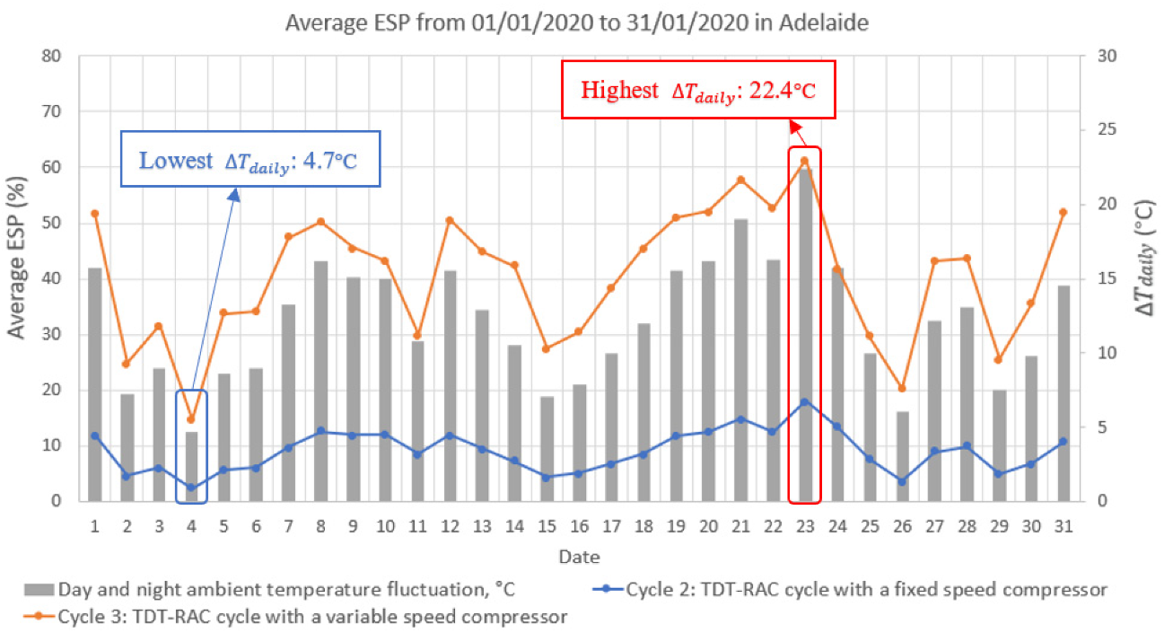
• The case study shows that, compared with the baseline cycle, the TDT-RAC cycle with a fixed speed compressor could, on average, save 2.4~18.1% energy, while the TDT-RAC cycle with a variable speed compressor could save 14.9~61.4% energy. Over the whole month, 9.1~40.4% energy can be saved by TDT-RAC cycles every day on average.

Based on this initial study on TDT-RAC systems/cycles, future investigations on this topic may include developing validated dynamic models for TDT-RAC systems rather than current cycle-based models in steady state. Detailed studies on the TDT itself may include understanding the water temperature profile and thermal stratification inside the TDT under different conditions.

8. Patents

Eric Jing Hu has patent “A HEAT TRANSFER ARRANGEMENT FOR IMPROVED ENERGY EFFICIENCY OF AN AIR CONDITIONING SYSTEM–A thermal ‘Diode Tank’” issued to AU 2014202998 Al.

References

- Sugarman, S.C. HVAC Fundamentals; River Publishers: Gistrup, Denmark, 2020; p. 509. [Google Scholar]
- Department of Climate Change and Energy Efficiency (DCCEE). Australia’s Emissions Projections, 2012; DCCEE: Canberra, Australia, 2012.
- Department of Industry, Science, Energy and Resources (DISER). Energy Update: Australian Energy Consumption and Production; DISER: Canberra, Australia, 2020.
- State of the Climate 2020: Bureau of Meteorology. Available online: http://www.bom.gov.au/state-of-the-climate/ (accessed on 23 September 2021).
- Head, L.; Adams, M.; McGregor, H.V.; Toole, S. Climate change and Australia. Wiley Interdiscip. Rev. Clim. Chang. 2014, 5, 175–197. [Google Scholar] [CrossRef] [Green Version]
- Walsh, J.A. Obesity & the First Law of Thermodynamics. Am. Biol. Teach. 2013, 75, 413–415. [Google Scholar] [CrossRef]
- Kumbhar, A.; Gulhane, N.; Pandure, S. Effect of Various Parameters on Working Condition of Chiller. Energy Procedia 2017, 109, 479–486. [Google Scholar] [CrossRef]
- Qiao, Z.; Long, T.; Li, W.; Zeng, L.; Li, Y.; Lu, J.; Cheng, Y.; Xie, L.; Yang, L. Performance assessment of ground-source heat pumps (GSHPs) in the Southwestern and Northwestern China: In situ measurement. Renew. Energy 2020, 153, 214–227. [Google Scholar] [CrossRef]
- Girard, A.; Gago, E.J.; Muneer, T.; Caceres, G. Higher ground source heat pump COP in a residential building through the use of solar thermal collectors. Renew. Energy 2015, 80, 26–39. [Google Scholar] [CrossRef]
- Christodoulides, P.; Aresti, L.; Florides, G. Air-conditioning of a typical house in moderate climates with Ground Source Heat Pumps and cost comparison with Air Source Heat Pumps. Appl. Therm. Eng. 2019, 158, 113772. [Google Scholar] [CrossRef]
- HZhang You, S.; Yang, H.; Niu, J. Enhanced performance of air-cooled chillers using evaporative cooling. Build. Serv. Eng. Res. Technol. 2016, 21, 213–217. [Google Scholar] [CrossRef]
- Wang, T.; Sheng, C.; Nnanna, A.A. Experimental investigation of air conditioning system using evaporative cooling condenser. Energy Build. 2014, 81, 435–443. [Google Scholar] [CrossRef]
- Yu, F.W.; Chan, K.T. Application of Direct Evaporative Coolers for Improving the Energy Efficiency of Air-Cooled Chillers. J. Sol. Energy Eng. 2005, 127, 430–433. [Google Scholar] [CrossRef]
- Waly, M.; Chakroun, W.; Al-Mutawa, N.K.; Al-Mutawa, N.K. Effect of pre-cooling of inlet air to condensers of air-conditioning units. Int. J. Energy Res. 2005, 29, 781–794. [Google Scholar] [CrossRef]
- Chen, X.; Chen, Y.; Deng, L.; Mo, S.; Zhang, H. Experimental verification of a condenser with liquid–vapor separation in an air conditioning system. Appl. Therm. Eng. 2013, 51, 48–54. [Google Scholar] [CrossRef]
- Zhong, T.; Ding, L.; Chen, S.; Chen, Y.; Yang, Q.; Luo, Y. Effect of a double-row liquid–vapor separation condenser on an air-conditioning unit performance. Appl. Therm. Eng. 2018, 142, 476–482. [Google Scholar] [CrossRef]
- Yang, J.; Chan, K.; Wu, X.; Yu, F.; Yang, X. An analysis on the energy efficiency of air-cooled chillers with water mist system. Energy Build. 2012, 55, 273–284. [Google Scholar] [CrossRef]
- Sözen, A.; Filiz, Ç.; Aytaç, I.; Martin, K.; Ali, H.M.; Boran, K.; Yetişken, Y. Upgrading of the Performance of an Air-to-Air Heat Exchanger Using Graphene/Water Nanofluid. Int. J. Thermophys. 2021, 42, 35. [Google Scholar] [CrossRef]
- Dobre, T.; Pârvulescu, O.C.; Stoica, A.; Iavorschi, G. Characterization of cooling systems based on heat pipe principle to control operation temperature of high-tech electronic components. Appl. Therm. Eng. 2010, 30, 2435–2441. [Google Scholar] [CrossRef] [Green Version]
- Zohuri, B. Basic Principles of Heat Pipes and History. Heat Pipe Des. Technol. 2016, 3, 1–41. [Google Scholar] [CrossRef]
- Moran, M.J.; Shapiro, H.N. (Eds.) A Review of: Fundamentals of Engineering Thermodynamics, 2nd ed.; John Wiley & Sons: Chichester, UK, 1993; Volume 18, p. 215. ISBN 0471592757. [Google Scholar] [CrossRef]
- Sound Energy: Compressor Speeds and What They Mean. Available online: https://soundenergycorp.com/about-us/blog/compressor-speeds-and-what-they-mean/ (accessed on 24 November 2021).