Probability-Based Customizable Modeling and Simulation of Protective Devices in Power Distribution Systems ^†

Abstract

Fused contactors and thermal magnetic circuit breakers are commonly applied protective devices in power distribution systems to protect the circuits when short-circuit faults occur. A power distribution system may contain various makes and models of protective devices, as a result, customizable simulation models for protective devices are demanded to effectively conduct system-level reliable analyses. To build the models, thermal energy-based data analysis methodologies are first applied to the protective devices’ physical properties, based on the manufacturer’s time/current data sheet. The models are further enhanced by integrating probability tools to simulate uncertainties in real-world application facts, for example, fortuity, variance, and failure rate. The customizable models are expected to aid the system-level reliability analysis, especially for the microgrid power systems.

1. Introduction

Protective devices prevent power devices in modern power generation, transmission, and distribution systems from thermal damage caused by overcurrent situations. Thermal magnetic circuit breakers (TMCB) and fused-contactors are the most commonly seen protective devices in medium–low-voltage level power distribution systems.

A contactor is an electrically controlled switch gear. Contactors are not designed to interrupt an overcurrent. Therefore, a fuse and contactor combination can serve as both a switch gear and a power protective device. Fuses act as sacrificial protective devices against overcurrent faults in AC and DC electronic circuits, and are widely applied in modern power systems, such as distribution feeders, transformers, induction motors, and heaters. Fuses have demonstrated simple structures, fast responses, and economic and reliable performance characteristics [1]. Under normal operating conditions, a fuse has a very small and negligible resistance in an electric circuit. When a short-circuit fault occurs, the fuse will heat up and start to melt, and a gap will be generated in between two ends of the fuse. The gap will generate an arc current, which will further melt the fuse. As the gap enlarges, the arc is weakened until the two ends are fully isolated.

Circuit breakers are designed to automatically protect the electrical circuit when the overcurrent or short-circuit fault occurs [1]. Unlike fuses, a circuit breaker can be manually or automatically reset after being triggered to resume normal operation [2]. When a fault occurs, the contacts in a circuit breaker will separate and, thus, interrupt the fault current. In this process, the metal contacts carry the currents, so an arc is established when they begin to separate. The mechanism inside the circuit breaker elongates the arc and extinguishes it. In today’s market, various types of circuit breakers, with different sizes, operating principles, and targeting current levels, are designed and produced. Among all of the types of circuit breakers, thermal magnetic circuit breakers (TMCB) are the most important in medium–low-voltage power distribution systems. The TMCBs are designed to instantaneously cut off high current level faults. A magnetic repulsion or an electromagnet mechanism separates the contacts as soon as the fault current exceeds the preset limit within an extremely short responding time (usually less than 2 ac cycles). On the other hand, the TMCBs allow smaller overloads (commonly in the range of 105% and 1000% of the rated current [1]) to exist for a longer time. The lower-level overcurrent heats up the bimetal in the circuit breaker; the thermal energy accumulates and the bimetal deflects, unlatches the mechanism, and mechanically isolates the circuit.

The power distribution system directly connects the power clients, distributed energy sources, and power distribution network. Routine maintenance of power components is required in power systems to ensure power quality, safety, and security. Since the power distribution systems usually contain a huge number of protective devices [3], there is a need to reduce the maintenance workload [4]. In recent years, simulation-based power system reliability analyses have shown promising savings in maintenance workloads [5,6]. To conduct such an analysis, the very first step is to construct accurate simulation models for the protective devices [7].

In the data sheet provided by the manufacturer, trip curves that plot tripping times versus current levels represent the operation characteristics of fuses. The voltage and current characteristics under fault situations were first observed by actually blowing the fuses [8]. Later, in [9], Tanaka et al. developed a fuse model to calculate the melting time and current from the joule-integral provided by the manufacturer. In one of our recent works [10], we used sampling, variance, and a residual sum of the squares analysis method to construct an optimized fuse model. More recently, reference [11] used the finite element analysis method to simulate the heating process of the fuses, and reference [12] used the $I^{2}t$ relationship to model, the time/current curve (TCC) provided by the manufacturer.

Similar TCCs are usually also provided in the data sheet of the circuit breakers. For TMCBs, the trip curve looks like an “L” shape, which consists of two parts: thermal tripping and magnetic tripping. The thermal tripping mode shares a common principle with the fuses: a curve that records the current levels and their corresponding time for heating up and separating the contacts. It is worthy to point out that a typical thermal trip curve displays as a performance band that is bound by minimum and maximum clearing times at different current levels (see [13] as an example). In reference [14], Robbins used a single curve, which was located in the middle of the performance band, to simplify the modeling procedure. Later, the authors of reference [15] studied the dynamics of the arc in the chamber of a low-voltage circuit breaker. Paper [10] studied the manufacturer’s TCC to simulate the thermal tripping of TMCB. More recently, reference [16] employed the thermal analysis method to build a dynamical model for the bimetallic strip in the TMCB. Paper [17] used the finite element analysis method to simulate the heating process of the circuit breaker.

From the literature, it is clear that the heating process of the fuse and the bimetal in TMCB share a similar mechanism. However, the exact melting time of the fuse and the thermal tripping time of the TMCB can be a random variable. As can be found from the manufacturer’s data, for example, references [13,18], two TCCs (sometimes known as minimum and maximum or total clearing time) are usually provided. This implies that, for a same make and model fuse, or TMCB, under a same current level, the reacting time may vary from time-to-time. Such randomness introduces uncertainties in system level reliability analysis and, therefore, must be considered in the modeling process.

In this work, we are interested in building simulation models for the protective devices in power distribution systems. This thermal energy-based analysis methodology is built on the basis of the TCC from the fuse/TMCB manufacturers. To show real-world performance and challenges of power protective devices, this new methodology presents uncertainty characteristics, for example, individual diversity, fortuity, and failure rate of the tripping performance. In addition, the new methodology is customizable; that is, the model can be easily tuned to simulate a practical device by using the manufacturer’s data. The rest of this paper is organized as follows: Section 2 reviews some preliminaries and operating principles of the protective devices. Section 3 discusses the detailed probability-based modeling process of the protective devices. Customizable examples are given in Section 4 for the purpose of illustration and validation. Our conclusions are drawn in Section 5.

2. Preliminaries

In this section we review some preliminaries that support the development of simulation models of the most commonly-seen protective devices in power distribution systems: fused contactors, and circuit breakers.

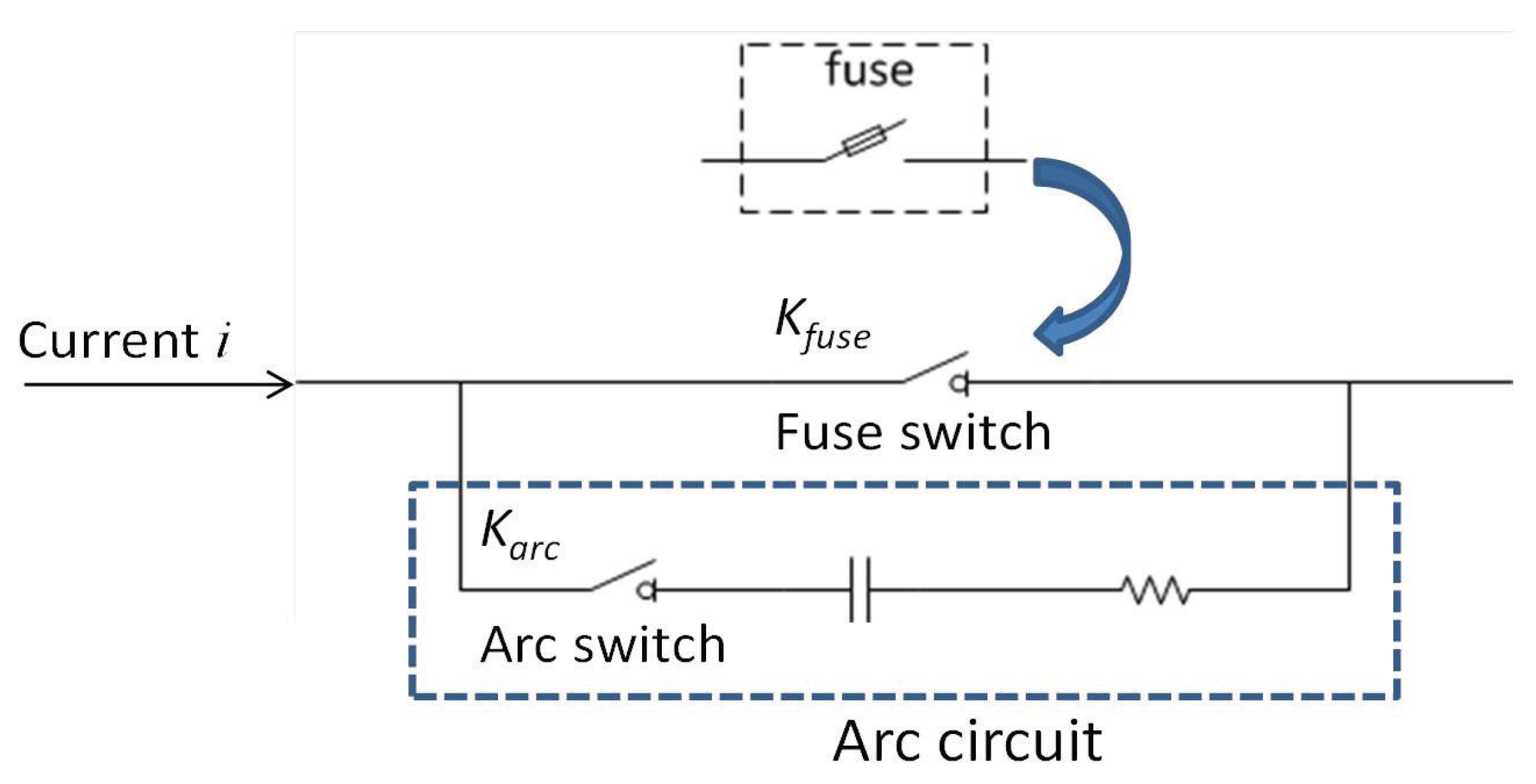
2.1. Fused Contactors

A contactor is an electrically controlled mechanical switch that is used in various implementations where large currents can occur, for example, the starting of electrical motors. An input voltage is required by the contactor to serve as a power supply. Optionally, the control of the contactor can be achieved by using an electrical control signal, for example, a programmable logic controller interface instead of the input voltage [19]. In this work, we use an ideal switch to simplify the contactor in the fuse–contactor combination model.

When a short-circuit fault occurs in the downstream circuit of the fuse, the current through the fuse increases sharply, and excesses the fuse-rated current. Then the internal joule heat increases and heats up the fuse. When the stored heat exceeds the melting threshold, the fuse melts and an arc is generated between the broken nodes. The melting time is defined as a time period between the occurrence of the fault and the fault current reaches the threshold. Immediately after that, the distance between two broken nodes extends, and through the current during the arcing process decreases fast, and finally it reaches zero when the arc extinguishes.

Based on the findings on the fuse melting process, we create an equivalent circuit for the fuse, as shown in Figure 1. The fuse switch is closed ($K_{fuse}=1$) and the arc switch remains open ($K_{arc}=0$) under normal operating conditions; thus, the fuse works as a shorted wire with negligible resistance. As the fuse melts, the fuse switch opens ($K_{fuse}=0$) and the arc switch closes ($K_{arc}=1$). The arc switch will again open ($K_{arc}=0$) when the current reaches zero. On the other hand, if the fault is instantaneous, and self-cleared before the fuse melts, the stored heat shall be released, and the fuse remains in normal operating status.

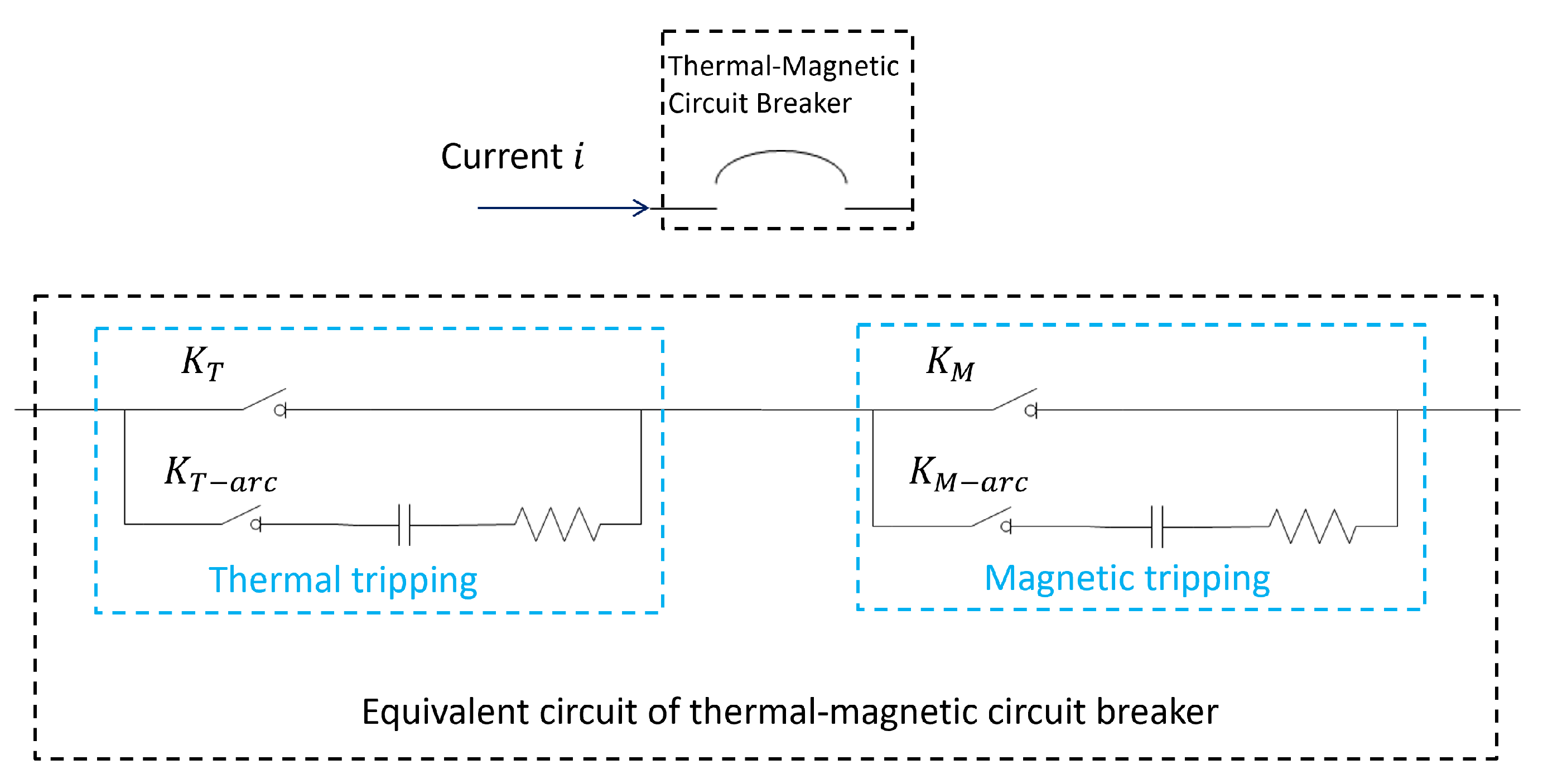
2.2. Thermal-Magnetic Circuit Breakers

Following the operational principle of TMCBs, an equivalent circuit is described in Figure 2, the switches $K_T$ and $K_M$ are both closed, and the switches $K_{T-arc}$ and $K_{M-arc}$ are both open under normal operating status. Thus, the circuit breaker works as a shorted wire with negligible resistance. As thermal tripping occurs, the switch $K_T$ opens and the switch $K_{T-arc}$ closes, while switches $K_M$ and $K_{M-arc}$ keep their original status. The switch $K_{T-arc}$ opens once again when the current reaches zero. During the thermal tripping, if the fault or the overload is instantaneous, and self-cleared before the internal heat energy exceeds the threshold that deflects the bimetal, the accumulated internal energy shall be released, and the circuit breaker remains in normal operating status. On the other end, when a fault current level is high enough to trigger the magnetic tripping mechanism, the switch $K_M$ opens and $K_{M-arc}$ closes immediately. The switch $K_{M-arc}$ opens once the current reaches zero. During the magnetic tripping process, switches $K_T$ and $K_{T-arc}$ keep their original status.

The melting process of the fuse shares a same principle with the thermal tripping process of the TMCBs. Some details of this process are discussed in the following remarks.

Remark 1.

The energy that heats up the fuse and/or the TMCB is known as the integral energy, which can be calculated using the following equation:

$$E={\int }_{t_0}^{t_1}{i}^2\left(t\right)dt$$

(1)

where $t_0,t_1$ are the time stamps when the current exceeds the rated current and when the integral energy calculation stops (i.e., fuse melts, thermal protection trips, or fault cleared), respectively. $T_h=t_1-t_0$ is known as the heating time. The fault current $i\left(t\right)$ may be a function of time rather than a constant.

Remark 2.

$E_C$ is known as the catalog energy of melting the fuse and the thermal tripping of the TMCB, which could be calculated by the following equation

$$E_C=I_C^2{T}_C$$

(2)

where $I_C,T_C$ are the catalog current and melting/thermal tripping time, respectively, which can be found in the manufacturer’s data sheet.

Remark 3.

In the arcing period, the current could be calculated as

$$i\left(t\right)=I_0{e}^{-\frac{t}{RC}}$$

(3)

where $I_0$ is the current when the arc is initially established. Its maximum value can be calculated as $I_0=\frac{V}{R_s}$, where $R_s$ is the resistance of the short circuit. When the bimetal begins to separate, the current will start to drop along with the increase of time t in Equation (3). Thus, the value of RC could be calculated by giving the arcing time and $I_0$.

3. Probability-Based Modeling of Protective Devices

In this section, we discuss the detailed process of constructing the customizable models of the protective devices using the manufacturer’s data sheet. With the probability-based modeling of the protective devices, the actual response time to clear a fault will become a dynamic value determined by a customized probability distribution, rather than a constant value in conventional modeling methods. The proposed customizable model will lead to a more realistic model that reflects real-world phenomenon in power delivery systems.

Before moving along to the modeling process, we hereby propose an assumption.

Assumption 1.

For a short-duration and self-cleared faults or transient overloads, which disappear before the integral energy exceeds the catalog energy, the time to release the stored heat is omitted in this study. Thus, the energy stored in the fuse and/or the TMCB will be set to zero immediately once the fault is self-cleared.

3.1. Probability-Based Thermal-Energy Analysis

We divide the thermal energy analysis into two steps. The first step is to obtain the mathematical model of the catalog energy from the manufacturer’s data by using data analysis methods. The second step is to integrate probability tools to reflect uncertainties in real-world application scenarios.

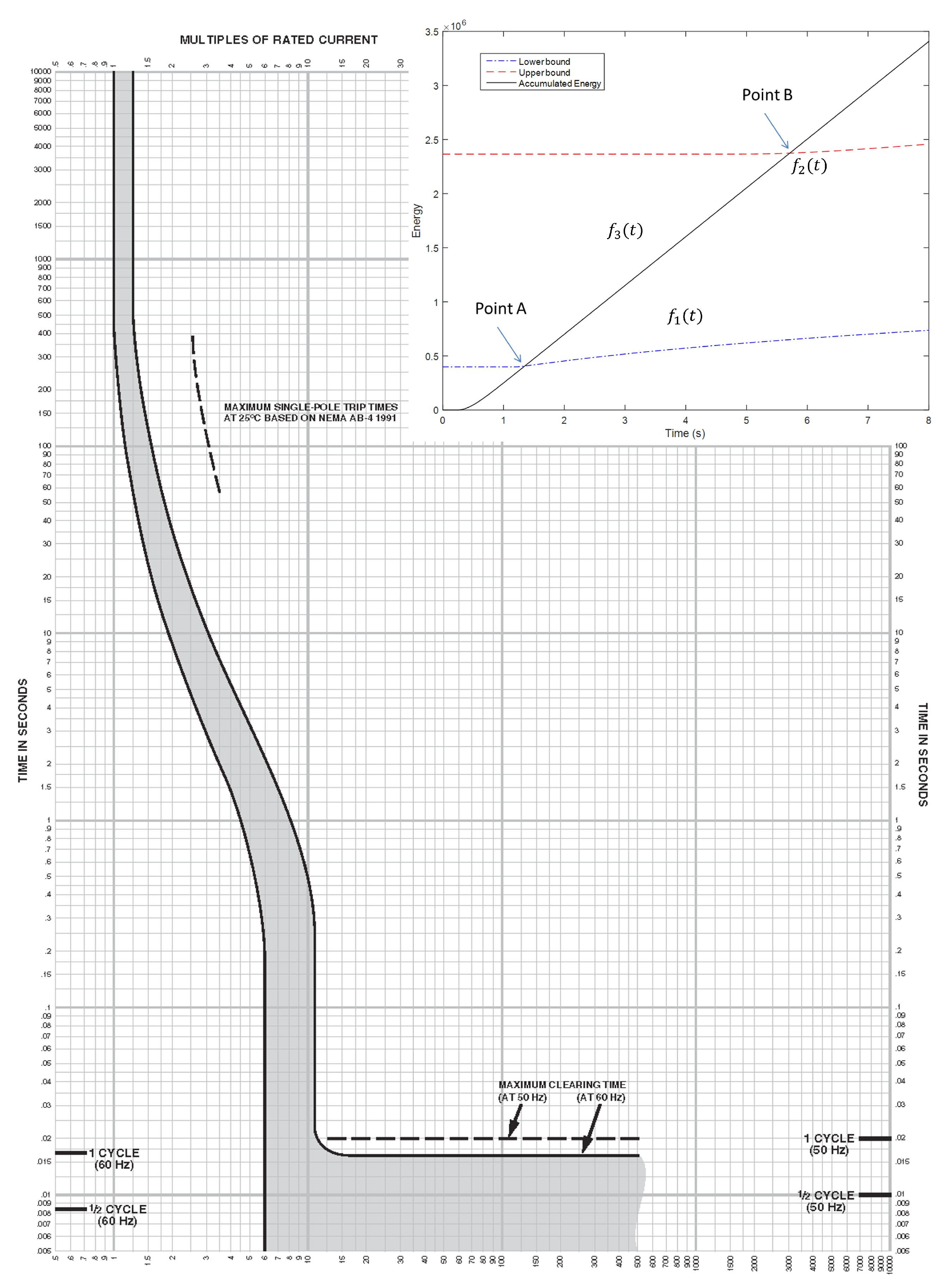
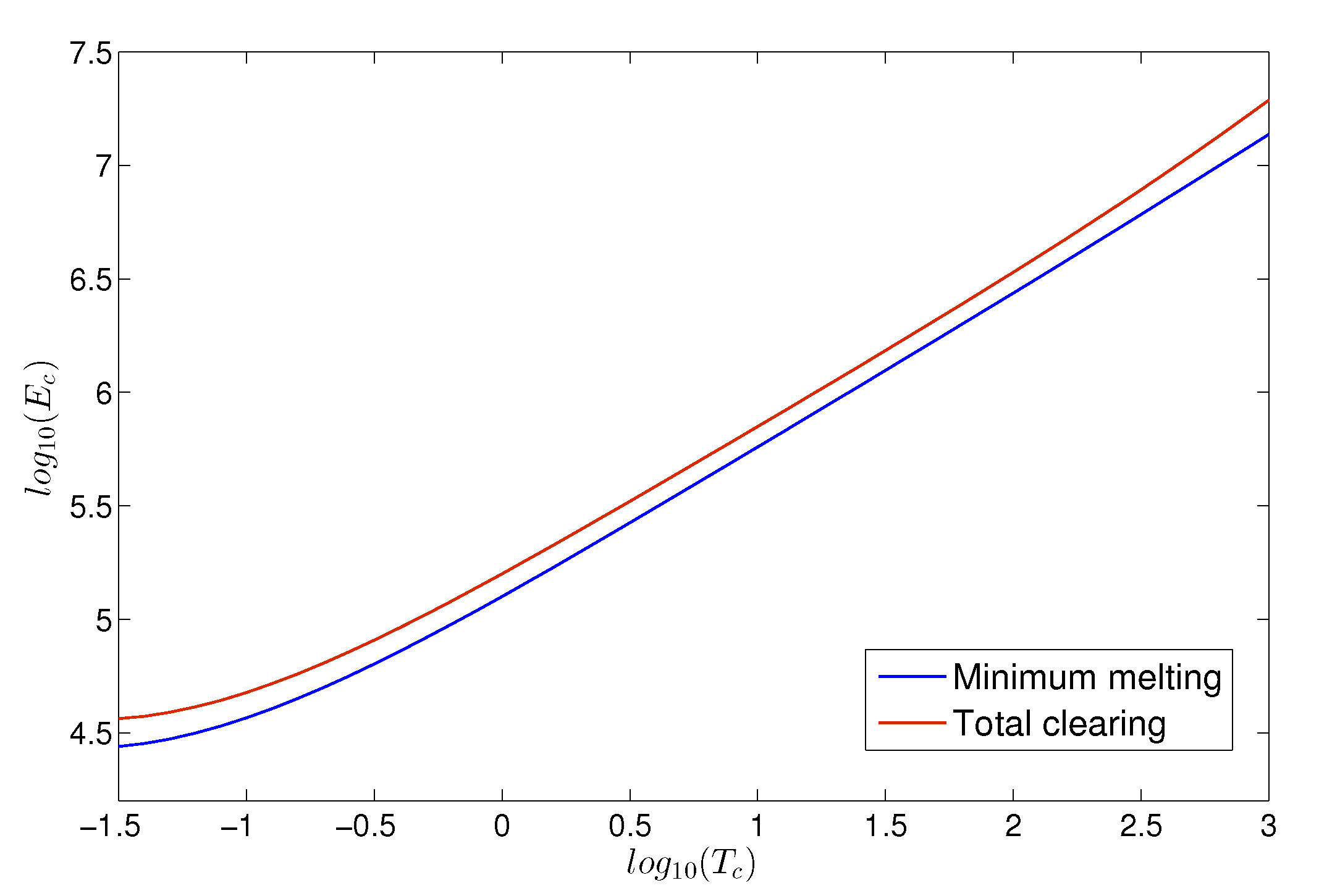
3.1.1. Curve Fitting and Data Analysis on Time/Current Curve

We start with obtaining an equation that describes the catalog energy. The catalog energy is usually not included in the manufacturer’s data sheet. Instead, the time current curve (TCC) is usually provided. Thus, a change of coordinates that transforms the time/current relation to time/energy relation must be performed based on Equation (2).

The second step is to choose an appropriate mathematical model to fit the curve. Based on the results from [10], we chose the polynomial model for the regression process. To pick the most optimal order for the polynomial regression model, we computed the residual sum of squares (RSS) for each order. The RSS serves as a criterion of optimality in the coefficient selection to evaluate the performance of each order of the polynomial. RSS calculates the deviations of the predicted from actual empirical values of data, which is an appropriate evaluation to measure the discrepancy between the data and an estimation model. The model with a smaller RSS fits the data better.

The RSS can be calculated using the following equation:

$$\mathrm{RSS}=\sum _{i=1}^n{(E_{c_i}-f\left(T_{c_i}\right))}^2,$$

(4)

where n is the samples size, $E_{c_i}$ is the i-th value of the catalog energy, and $T_{c_i}$ is the i-th value of the melting time for a certain number of randomly picked testing data out of the total samples obtained in the first step. The polynomial function $f\left(T_{c_i}\right)$, which is regressed from the remaining samples, is used to estimate the catalog energy given by

$$f\left(T_{c_i}\right)={\widehat{E}}_{c_i}=a_0+a_1{T}_{c_i}+\dots +a_k{T}_{c_i}^k,$$

(5)

where $a_0,\dots ,a_k$ are polynomial coefficients.

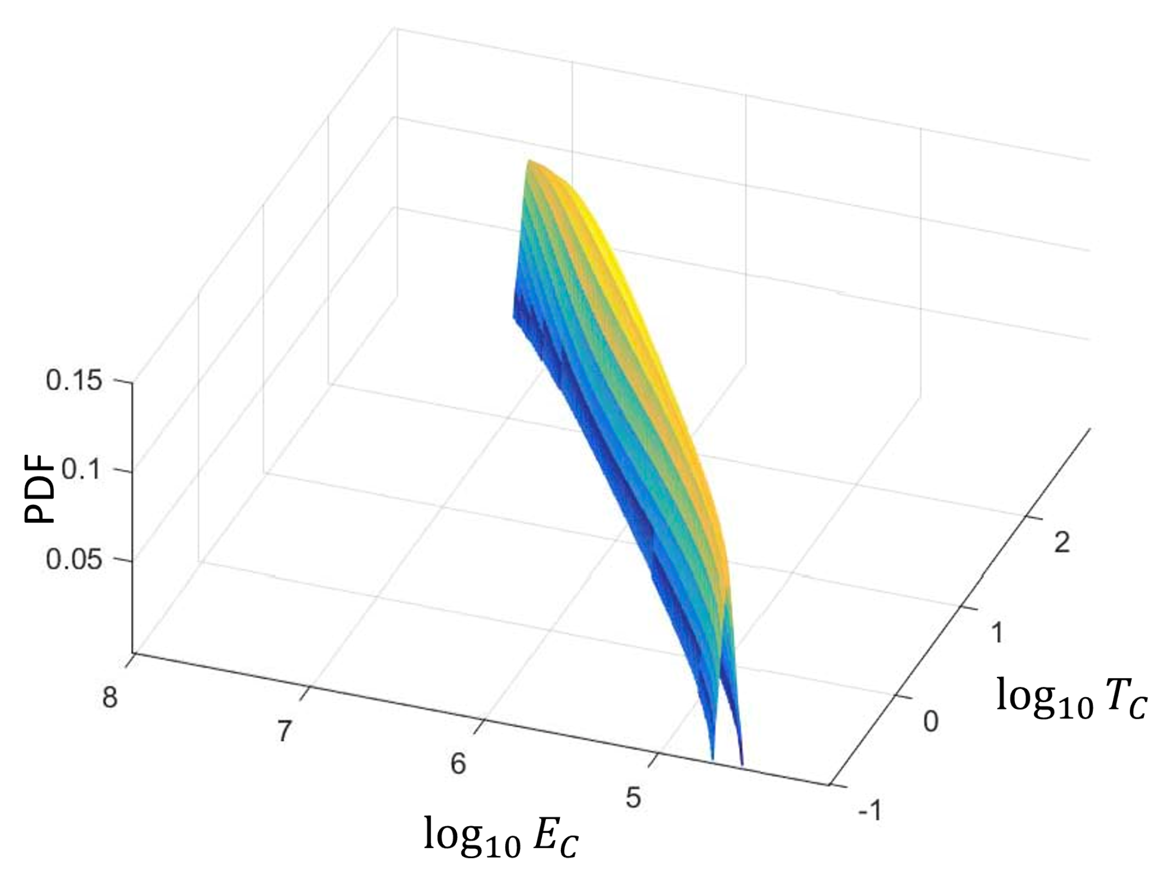
3.1.2. Probability Integrated Modeling

When a fault occurs, the fault current will exceed the rated current of the fuse quickly. After this, the heat energy will start to accumulate, and the exact melting/thermal-tripping time should fall into a time interval, which is regulated by the upper- and lower-boundary of the catalog energy with respect to time. We use Figure 3 to make the demonstration easier to understand (here we use the TCC of Square D QOB-3100 Circuit Breaker [18] as an example).

From the manufacturer’s TCC data sheet, we can obtain two curves regarding to the catalog energy by taking a change of coordinates using Equations (2) and (5). The lower-boundary curve, i.e., $f_1\left(t\right)$, is based on the “minimum clearing time”, and the upper-boundary curve, i.e., $f_2\left(t\right)$, can be obtained from the “maximum clearing time”. When a fault occurs, by (1), the accumulative energy ($E_m$) curve, denoted as $f_3\left(t\right)$, will cross $f_1\left(t\right)$ and $f_2\left(t\right)$. Denoting these two intersections as Point A and Point B in Figure 3, we can find the time stamps of these two points as $t_1$ and $t_2$, respectively. Assume the probability of melting/thermal-tripping in the time period of $t\in [t_1,t_2]$ follows a normal distribution, which is a reasonable and often-seen assumption in industrial applications and standards, we can then calculate the probability density function (PDF) at each time point in between $t_1$ and $t_2$. It is noted that in case some application scenarios may not follow normal distribution, the PDF can be replaced by the appropriate distribution.

We calculate the mean value of this normal distribution by using the average of the lower-boundary and upper-boundary functions as follows:

$$\mu \left(t\right)=\mathrm{Average}(f_1\left(t\right),f_2\left(t\right)).$$

(6)

The standard deviation of this distribution can be calculated as:

$$\begin{array}{cc}\hfill \sigma \left(t_i\right)& =\frac{\Delta f_2\left(t\right)-\Delta f_1\left(t\right)}{2\times Z_{\alpha /2}}\hfill \\ \hfill & =\frac{(f_2\left(t_i\right)-f_1\left(t_i\right))-(f_2\left(t_{i-1}\right)-f_1\left(t_{i-1}\right))}{2\times Z_{\alpha /2}}\hfill \end{array}$$

(7)

where $t_i$ is any given time stamp in the time period of $[t_1,t_2]$, $1-\alpha$ is the confidence level, and Z is the critical value, which can be searched from the standard normal table. By simply using the empirical rule, also known as the “68-95-99.7” rule, we can easily find out the Z value to be 2 and 3, for the commonly-used 5% and 0.3% failure rate.

Remark 4.

Determined by the quality of the fuse products in real-world application, the failure rate could be reduced to 0.3% or even lower. Therefore, the Z value in Equation (7) should be changed accordingly.

Therefore, the cumulative probability function that the fuse is triggered at a time stamp $t_i$ after the fault happens can be calculated as:

$$P\left(t_i\right)=\frac{{\int }_0^{t_i}\omega \left(t\right)dt}{{\int }_0^{\infty }\omega \left(t\right)dt},$$

(8)

where

$$\omega \left(t\right)=\frac{1}{2\sqrt{\pi }\sigma \left(t\right)}{e}^{\frac{f_3\left(t\right)-\mu \left(t\right)}{2{\sigma }^2\left(t\right)}}.$$

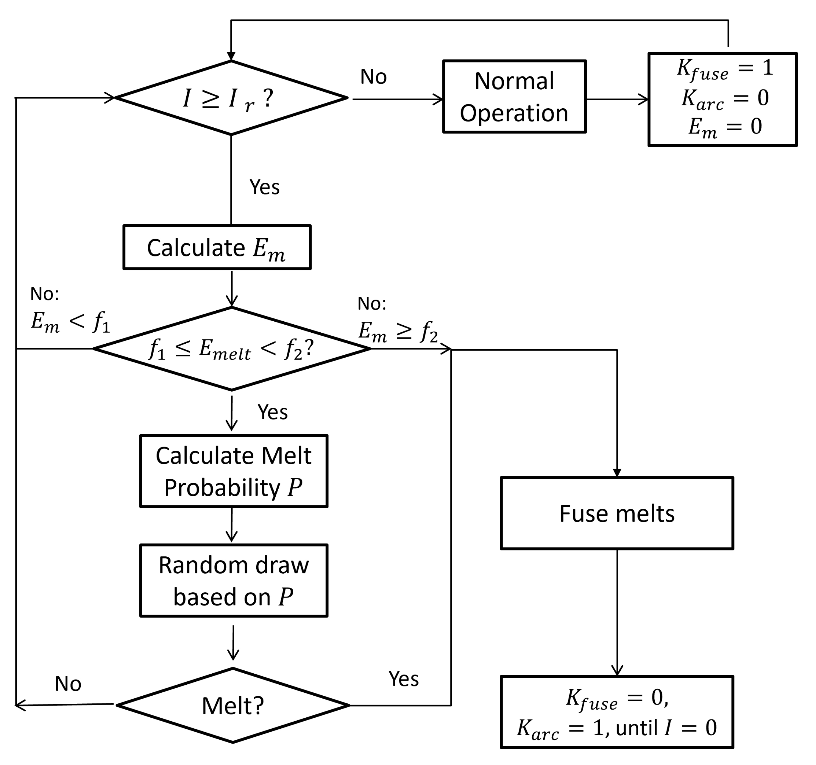
3.2. Customizable Fuse Modeling

Based on our previous discuss, the operation flow of the fuse model is summarized in Figure 4.

When a fault occurs, by (1), the integral energy ($E_m$) will rapidly accumulate, and after a certain period of time, the integral energy will exceed the lower-boundary (for example, it is denoted as the minimum clear time in [18]) of the catalog energy, i.e., $E_m\left(t\right)\ge f_1\left(t_1\right)$, where $t_1$ is the corresponding time stamp. From this time point, we consider there is a probability that the fuse will melt. Therefore, a random draw will be initiated based on this probability. If the result is “positive”, then we consider the fuse is melted, and the arcing procedure starts; if the result is “negative”, then the fuse is not melted, and this probability will increase with time following the PDF in (8), unless the fault is self-cleared. As integral energy reaches the upper-boundary (for example, it is denoted as the total clear time in [18]) of the catalog energy, i.e., $E_m\left(t\right)=f_2\left(t_2\right)$, we consider the melting probability increases to $100\%$, and the fuse must melt. It is worthy to point out that, due to the failure rate, we will allow the existence of outliers after the melting probability reaches 100%. Moreover, if the fault or overload current is self-cleared before the fuse melts, we consider the heat energy that stores within the fuse is released instantaneously based on Assumption 1.

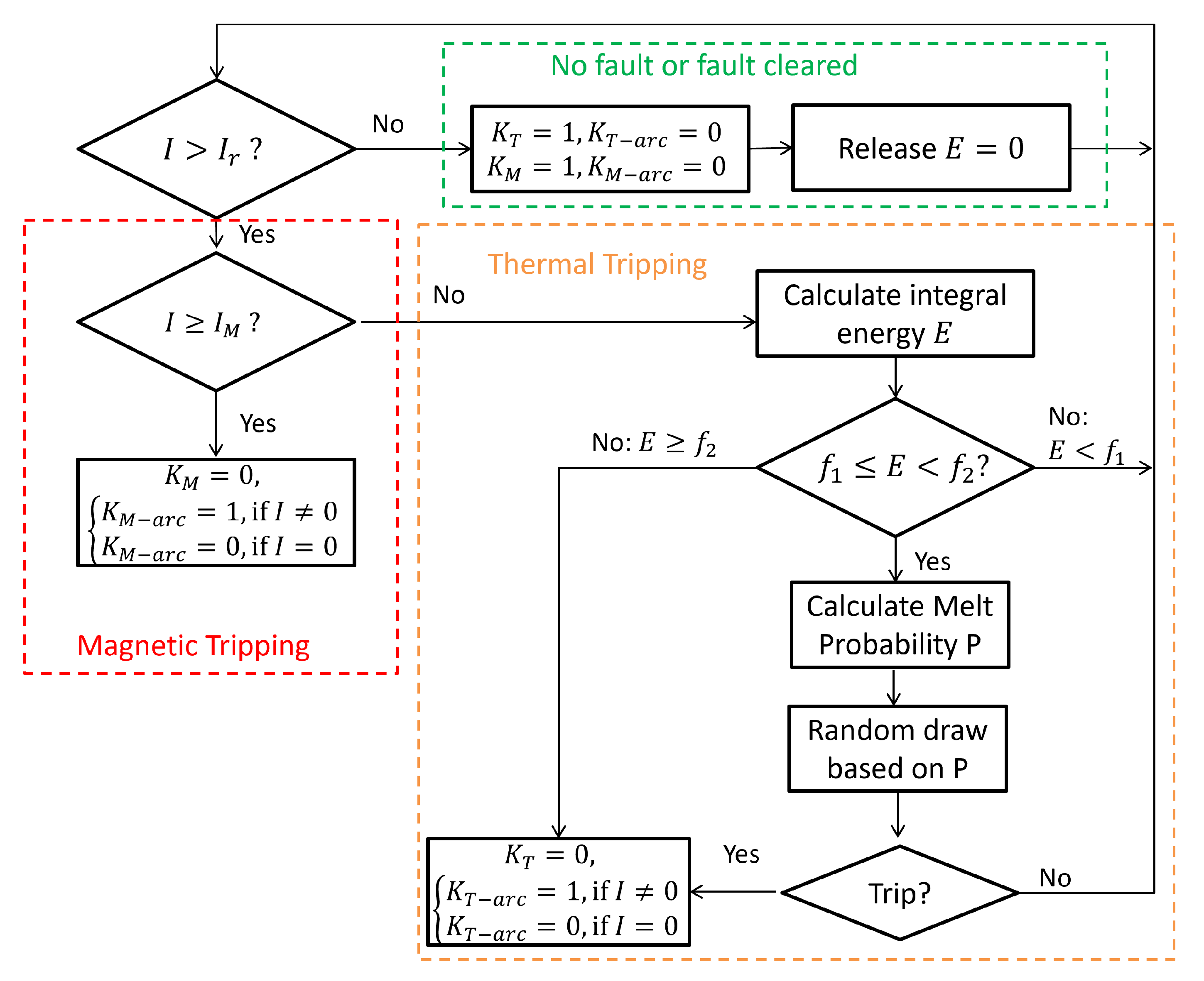
3.3. Customizable Thermal-Magnetic Circuit Breaker Modeling

A TMCB has two major protective functions: the thermal tripping and the magnetic tripping. Determined by the fault current level, either of these two functions may be triggered to cut off the faulty circuit and protect the power devices. An operational flow chart of the circuit breaker simulation model is therefore sketched in Figure 5.

When a fault happens, if the fault current exceeds the rated current, but stays below the magnetic tripping limit, i.e., $I_r<I<I_M$, then the thermal tripping will be activated. The heating process is essentially similar as melting the fuse: the internal joule heat increases as well to heat up the bimetal. When the integrated heat exceeds the lower-boundary ($f_1\left(t\right)$), (known as the minimum clearing time curve, see [13] as an example), the bimetal is heated and intend to be separated. The heating process has the same principle as fuse melting: a tripping probability will be generated based on Equation (8), and it increases as the heating continues. Whether the random draw based on the probability is a “positive” or the integrated heat exceeds the upper-boundary ($f_2\left(t\right)$) (known as the maximum clearing time curve in [13]), the thermal tripping is completed, bimetal is separated, and an arc is generated between the gap of the bimetal. Immediately after that, the distance between the two contacts of the bimetal extends to extinguish the arc. On the other hand, if the fault current exceeds the magnet tripping current limit, i.e., $I\ge I_M$, the contacts will be separated immediately.

4. Validation on Customized Model Examples

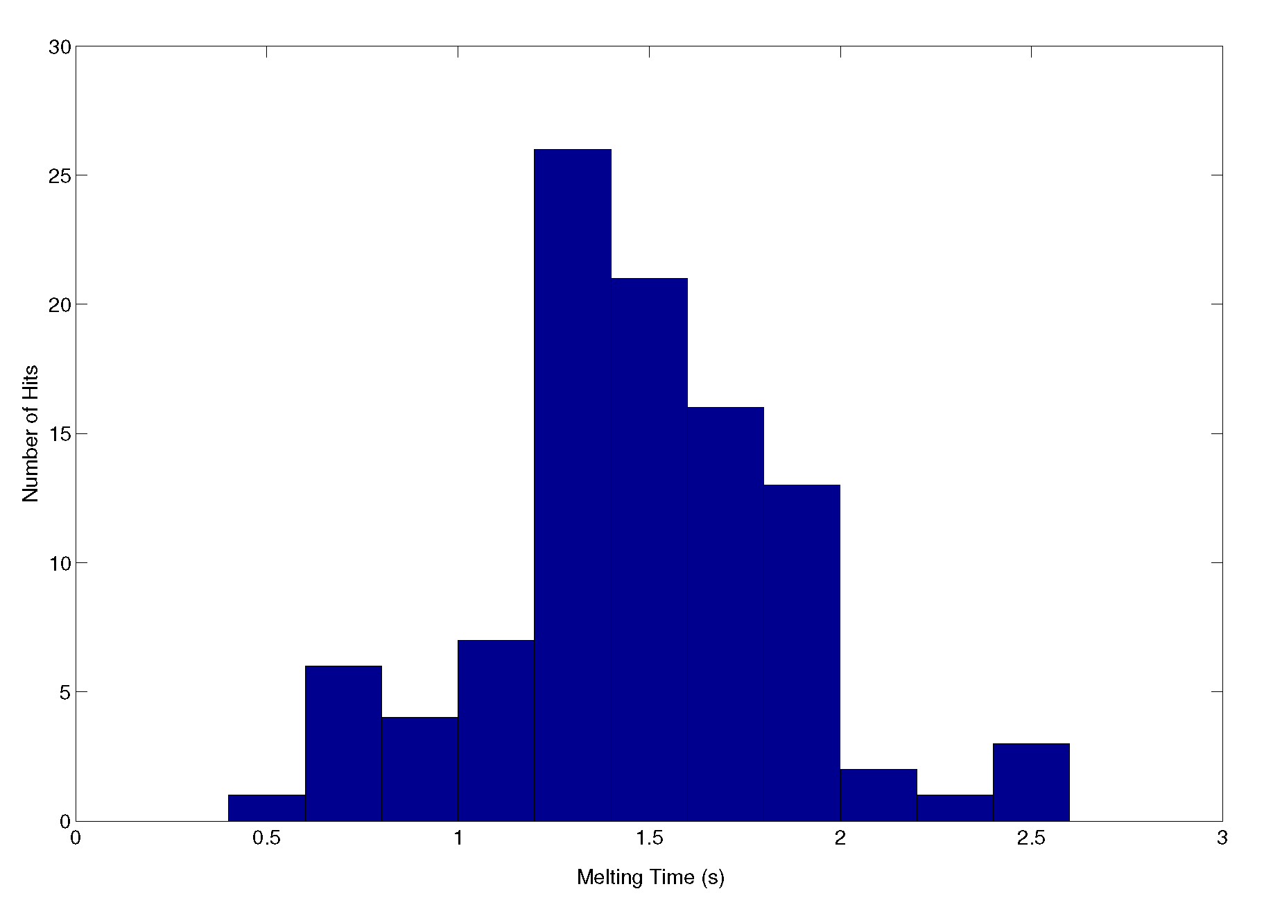
4.1. Customized Simulation Model of “EATON CLT-30A” Fuse

For test and verification purposes, we construct a simulation model for the “EATON CLT-30A” fuse, whose tripping curves are shown in [18].

We first took 30 samples evenly from each TCC, and applied Equation (2) to calculate the catalog energy $E_c$. Now the time/current relation has been transferred to time/energy relation. After this change of coordinates, we use data analysis and curve fitting methods to obtain the optimal expression of $E_c$, with the melting time $T_c$.

Secondly, we compare the RSS value from first order to ninth order, i.e., $k=1,\dots ,9$ (500 rounds of four-fold validation), by using Equation (4), where the sample size is 75. The RSS values are summarized in

Table 1. RSS comparison of polynomial regression model.

Minimum Melting Curve		Total Clearing Curve
Order	RSS	Order	RSS
1	85.00	1	23.99
2	16.54	2	2.71
3	6.90	3	1.37
4	1.15	4	0.23
5	0.64	5	0.20
6	0.82	6	0.21
7	0.92	7	0.27
8	16.33	8	0.54
9	29.0	9	0.67

.

It is clear that the fifth-order polynomial would be the most optimal order for the polynomial regression model because the RSS values reach their minimum points and start to increase after the sixth-order. Such an increase may be caused by overfitting.

Based on the above discussion, our final catalog energy/time equation that is extracted from the minimum melting TCC of fuse [18] can be written as

$$\begin{array}{cc}\hfill log{E}_c=& 5.077+0.631log{T}_c+0.052{log}^2{T}_c-0.032{log}^3{T}_c\hfill \\ \hfill +& 0.010{log}^4{T}_c-0.001{log}^5{T}_c;\hfill \end{array}$$

(9)

and the catalog energy/time equation from the total clearing TCC of fuse [18] is given by

$$\begin{array}{cc}\hfill log{E}_c=& 5.223+0.622log{T}_c+0.052{log}^2{T}_c-0.03{log}^3{T}_c\hfill \\ \hfill +& 0.011{log}^4{T}_c-0.001{log}^5{T}_c.\hfill \end{array}$$

(10)

These catalog energy/time curves of Equations (9) and (10) are plotted in Figure 6.

We chose a commonly-seen failure rate of 5% to the product as a demonstration; thus, we have a standard deviation $2\sigma$ added to both sides as $\left(f_2\left(t\right)-f_1\left(t\right)\right)/4$. Figure 7 shows the probability distribution of the fuse melting with its corresponding melting time and integral energy. It is noted that this distribution follows a normal distribution with respect to the Z axis.

Then, we put the fuse simulation model in a 2000-amp DC fault current environment, and then observe its melting time.

Figure 8 and Figure 9 shows a sample result from our customized model. The melting time of the fuse under a certain level of fault current will become a random variable that follows a customized distribution rather than just a constant.

To demonstrate the probability specifications, we repeated this test for 100 times, and the random sample of the fault clearing time is summarized in histogram and boxplot, as shown Figure 8 and Figure 9, respectively. It can be noticed that most of the melting times are concentrated in between 1.2 and 2 s, with a median of 1.42 s, which revealed the customized distribution characteristics. Among these 100 tests, 94 results hit the (0.7, 2.1) second time intervals, which can be found from the minimum and the total clearing times, respectively at 2000-amp, according to [18]. There were two trials where the fuse melted before 0.7 s, and four trials where the fuse melted after 2.1 s. The number of failed tests indeed matched our assumption of the $5\%$ failure rate.

4.2. Customized Simulation Model of “Square D QOB-3100” Circuit Breaker

We further constructed the simulation model for “Square D QOB-3100” [13], which is a type of TMCB that is used in power distribution panels. Since the sampling, curve fitting and regression procedure is essentially similar as in the previous example, these procedures were omitted in this example. We displayed the probability distribution model for the thermal-tripping function as shown in Figure 10.

Then, we put the customized model in a simulation testbed using MATLAB/Simulink. We deployed an induction motor in this testbed as shown in Figure 11. In this test, we attached an induction motor to the ac voltage source. The motor is set to start at $t=0.5$ s, and a short-circuit fault is set to occur at $t=1$ s. This type of TMCB has a rated current of 100 Amps. The TMCB allows a short-period overcurrent to pass; in this test, we observed two types of overcurrent: the inrush current when the motor starts and the fault current.

As can be seen in Figure 12, although the inrush current exceeds the rated current of this TMCB, its short lasting time (less that 0.2 s) cannot trigger the thermal tripping. The simulated three-phase fault then caused the thermal tripping, and the TMCB cleared the fault current within 3.8 s. According to [13], the thermal tripping time period at this current level $T_C\in [1.3,7.5]$ seconds. The simulation results has met the descriptions of the manufacturer’s data sheet [13] and, therefore, accurately shows the tripping characteristics.

5. Conclusions and Future Work

In this paper, we constructed customizable simulation models for the commonly-seen protective devices, fused contactors, and thermal magnetic circuit breakers, in power distribution systems. We applied a thermal energy-based analysis to the manufacturer’s time/current curves, and integrated probability tools to demonstrate real-world phenomena of the protective devices, such as individual variance, fortuity, and product failure. Thus, instead of using the conventional protective model, which simplifies the tripping time as a unified time point at a specified fault current level, by using the proposed method, we are enabled to prototype a more realistic performance of the power protection devices, and it may spot more potential issues in the power network. Additionally, the models are able to be customized to suit the characteristics of different models/makes of protective devices with different standards. This customizable model can be simply edited and applied to simulate various protective devices in power distribution systems. Looking forward, considering the protection coordination between protective devices, we will adopt the customizable models into our systematic power grid reliability appraisal platform to simulate specified power systems in the real-world.

References

1. Sheldrake, A. Handbook of Electrical Engineering: For Practitioners in the Oil, Gas, and Petrochemical Industry; Wiley: New York, NY, USA, 2013. [Google Scholar]
2. Holm, R. Electric Contacts: Theory and Application; Springer Science & Business Media: New York, NY, USA, 2013. [Google Scholar]
3. Feng, Y.; Zhou, X.; Krstic, S.; Zhou, Y.; Shen, Z.J. Molded Case Electronically Assisted Circuit Breaker for DC Power Distribution Systems. IEEE Trans. Power Electron. 2020, 36, 6586–6595. [Google Scholar] [CrossRef]
4. Yssaad, B.; Khiat, M.; Chaker, A. Reliability centered maintenance optimization for power distribution systems. Int. J. Electr. Power Energy Syst. 2014, 55, 108–115. [Google Scholar] [CrossRef]
5. Carnero, M.C.; Gómez, A. Maintenance strategy selection in electric power distribution systems. Energy 2017, 129, 255–272. [Google Scholar] [CrossRef]
6. Iberraken, F.; Medjoudj, R.; Medjoudj, R.; Aissani, D.; Haim, K.D. Reliability-based preventive maintenance of oil circuit breaker subject to competing failure processes. Int. J. Perform. Eng. 2013, 9, 495. [Google Scholar]
7. Lei, C.; Tian, W.; Zhang, Y.; Fu, R.; Jia, R.; Winter, R. Probability-based circuit breaker modeling for power system fault analysis. In Proceedings of the 2017 IEEE Applied Power Electronics Conference And Exposition (APEC), Tampa, FL, USA, 26–30 March 2017; pp. 979–984. [Google Scholar]
8. Robbins, T. Fuse model for overcurrent protection simulation of DC distribution systems. In Proceedings of the INTELEC’93, 15th International Telecommunications Energy Conference, Paris, France, 27–30 September 1993; Volume 2, pp. 336–340. [Google Scholar]
9. Tanaka, T.; Kawaguchi, H.; Terao, T.; Babasaki, T.; Yamasaki, M. Modeling of fuses for DC power supply systems including arcing time analysis. In Proceedings of the INTELEC 2007, 29th International Telecommunications Energy Conference, Rome, Italy, 30 September–4 October 2007; pp. 135–141. [Google Scholar]
10. Tian, W.; Lei, C.; Zhang, Y.; Li, D.; Fu, R.; Winter, R. Data analysis and optimal specification of fuse model for fault study in power systems. In Proceedings of the Power and Energy Society General Meeting (PESGM), Boston, MA, USA, 17–21 July 2016; pp. 1–5. [Google Scholar]
11. Szulborski, M.; Łapczyński, S.; Kolimas, Ł.; Kozarek, Ł.; Rasolomampionona, D.D.; Żelaziński, T.; Smolarczyk, A. Transient Thermal Analysis of NH000 gG 100A Fuse Link Employing Finite Element Method. Energies 2021, 14, 1421. [Google Scholar] [CrossRef]
12. Lee, S.Y.; Son, Y.K.; Cho, H.J.; Sul, S.K. Normalization of Capacitor-Discharge I2t by Short-Circuit Fault in VSC-Based DC System. IEEE Trans. Power Electron. 2021, 37, 843–854. [Google Scholar] [CrossRef]
13. QO and QOB Miniature Circuit Breaker Manual. Available online: https://download.schneider-electric.com/files?p_Doc_Ref=0730CT9801 (accessed on 22 December 2021).
14. Robbins, T. Circuit-breaker model for overcurrent protection simulation of DC distribution systems. In Proceedings of the INTELEC’95, 17th International Telecommunications Energy Conference, The Hague, The Netherlands, 29 October–1 November 1995; pp. 628–631. [Google Scholar]
15. Swierczynski, B.; Gonzalez, J.; Teulet, P.; Freton, P.; Gleizes, A. Advances in low-voltage circuit breaker modelling. J. Phys. D Appl. Phys. 2004, 37, 595. [Google Scholar] [CrossRef]
16. Čepon, G.; Starc, B.; Zupančič, B.; Boltežar, M. Coupled thermo-structural analysis of a bimetallic strip using the absolute nodal coordinate formulation. Multibody Syst. Dyn. 2017, 41, 391–402. [Google Scholar] [CrossRef]
17. Szulborski, M.; Łapczyński, S.; Kolimas, Ł.; Zalewski, D. Transient Thermal Analysis of the Circuit Breaker Current Path with the Use of FEA Simulation. Energies 2021, 14, 2359. [Google Scholar] [CrossRef]
18. CLT Fuses Manufacturer Data Sheet. Available online: https://www.eaton.com/content/dam/eaton/markets/for-safety-sake/files/current-limiting-fuses.pdf (accessed on 22 December 2021).
19. Sadowski, N.; Bastos, J.; Albuquerque, A.; Pinho, A.; Kuo-Peng, P. A voltage fed AC contactor modeling using 3D edge elements. IEEE Trans. Magn. 1998, 34, 3170–3173. [Google Scholar] [CrossRef]
Figure 1. Equivalent fuse circuit.
Energies 15 00199 g001
Figure 2. Equivalent circuit of TMCB.
Energies 15 00199 g002
Figure 3. The thermal tripping interval of the Square D QOB-3100 Circuit Breaker [18].
Energies 15 00199 g003
Figure 4. Operating flow chart of the probability-integrated fuse simulation model.
Energies 15 00199 g004
Figure 5. Operational flow chart of the probability-integrated TMCB model.
Energies 15 00199 g005
Figure 6. Catalog energy/time curves of obtained from manufacturer data.
Energies 15 00199 g006
Figure 7. Fuse Melting probability distribution of EATON CLT-30A fuse.
Energies 15 00199 g007
Figure 8. Histogram of a random sample of fault clearing time distribution of 100 trials.
Energies 15 00199 g008
Figure 9. Boxplot of a random sample of fault clearing time distribution of 100 trials.
Energies 15 00199 g009
Figure 10. Thermal tripping probability distribution of the “Square D QOB-3100” circuit breaker.
Energies 15 00199 g010
Figure 11. Simulation testbed for “Square D QOB-3100” circuit breaker.
Energies 15 00199 g011
Figure 12. Inrush and fault current (RMS) passing “Square D QOB-3100” circuit breaker.
Energies 15 00199 g012