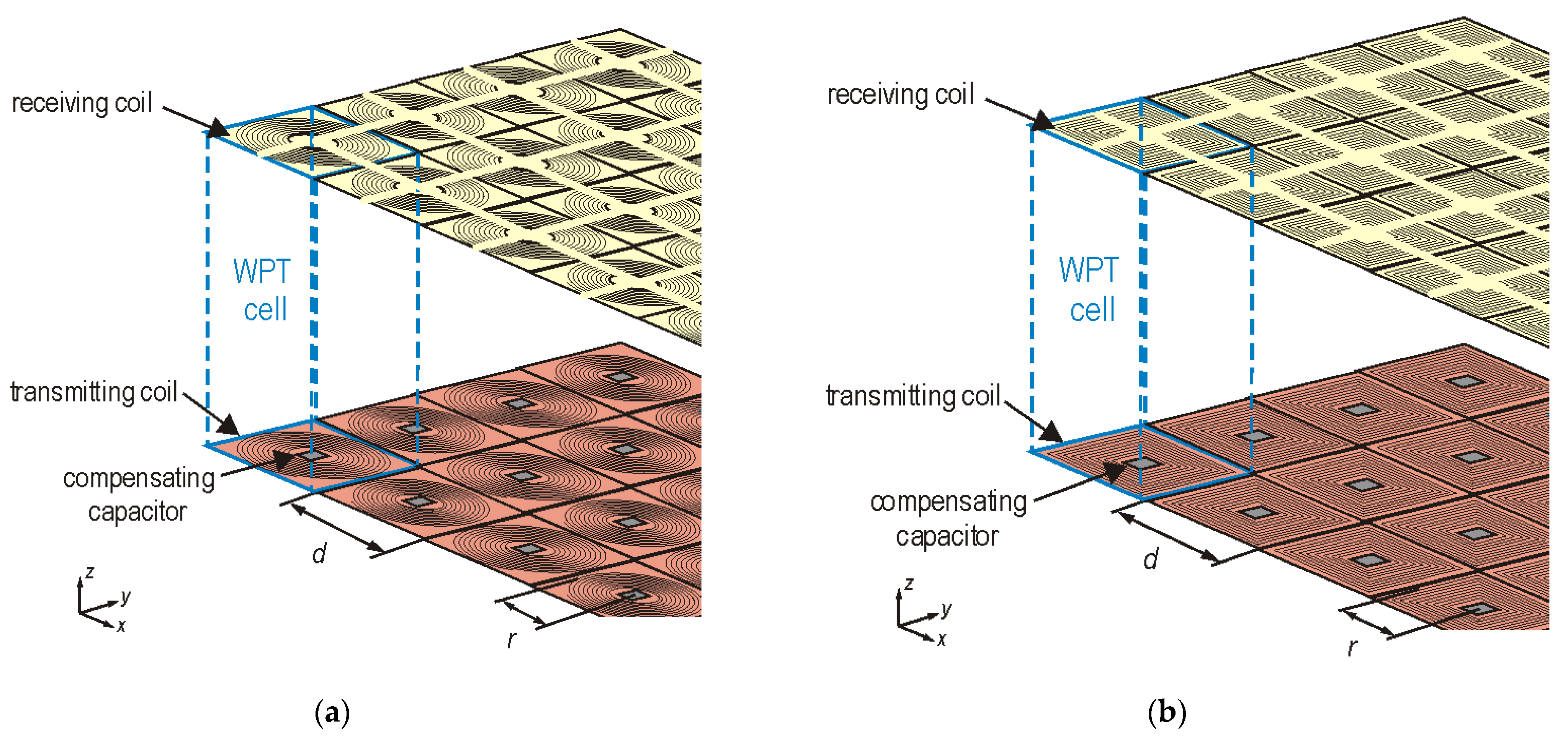
Figure 1.
The studied WPT system composed of: (a) circular planar coils, (b) square planar coils.
Figure 1.
The studied WPT system composed of: (a) circular planar coils, (b) square planar coils.
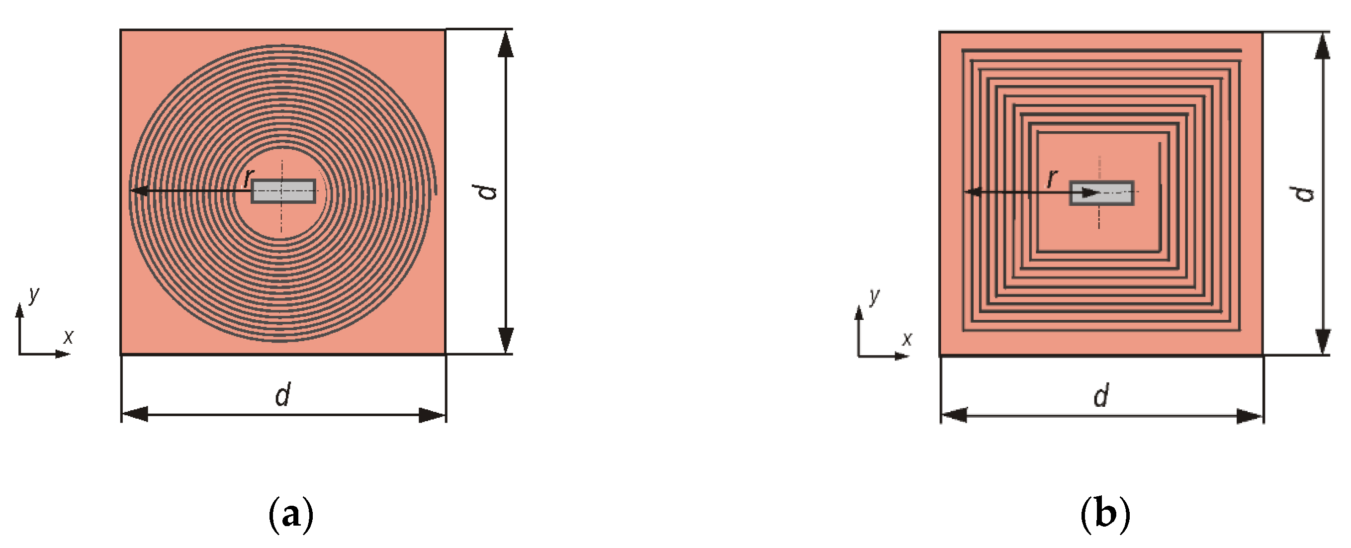
Figure 2.
Two types of modelled coils: (a) circular, (b) square.
Figure 2.
Two types of modelled coils: (a) circular, (b) square.
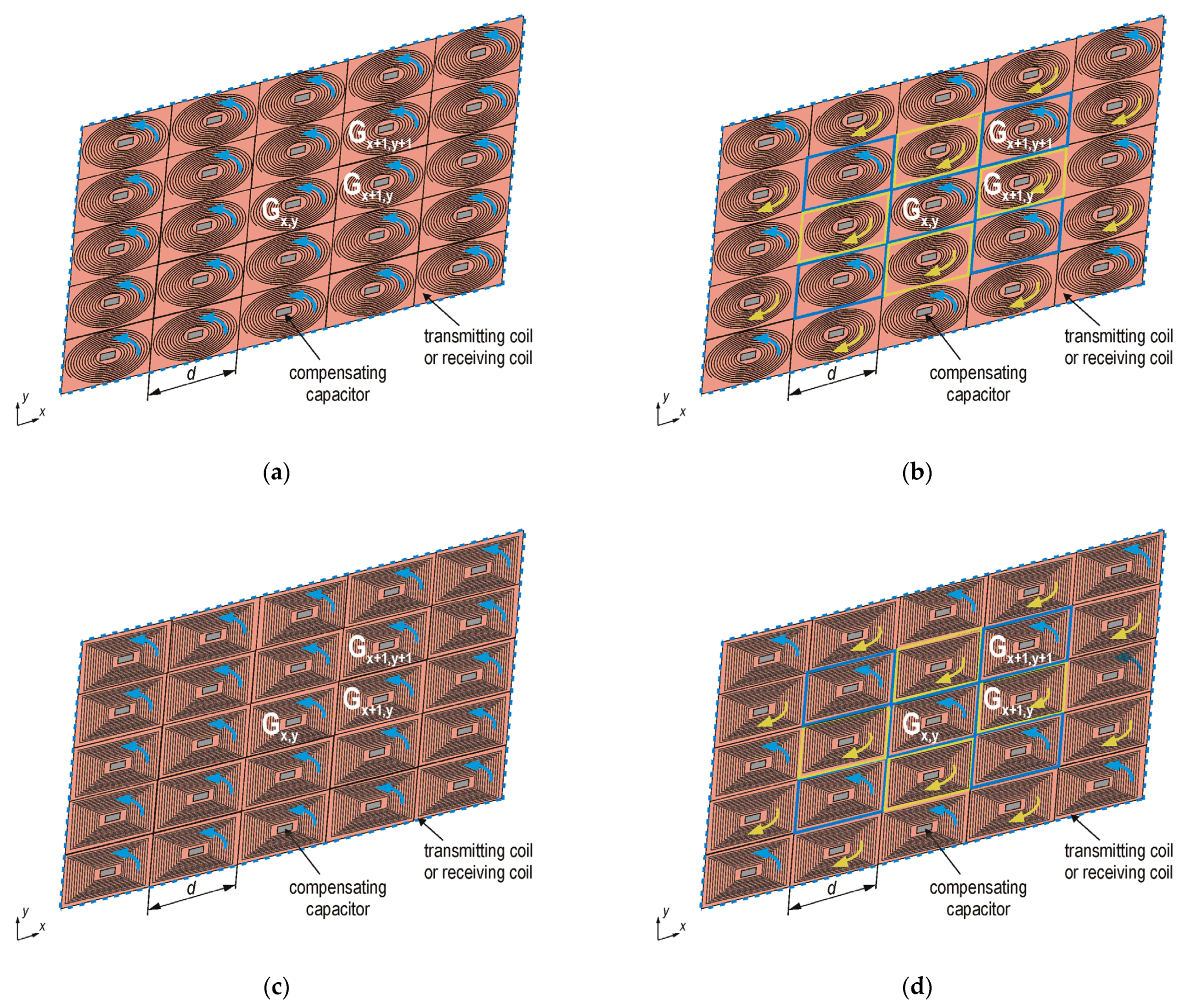
Figure 3.
The studied transmitting/receiving surface composed of: (a) circular coils with the same winding direction, (b) circular coils with the opposite winding direction, (c) square coils with the same winding direction, (d) square coils with the opposite winding direction.
Figure 3.
The studied transmitting/receiving surface composed of: (a) circular coils with the same winding direction, (b) circular coils with the opposite winding direction, (c) square coils with the same winding direction, (d) square coils with the opposite winding direction.
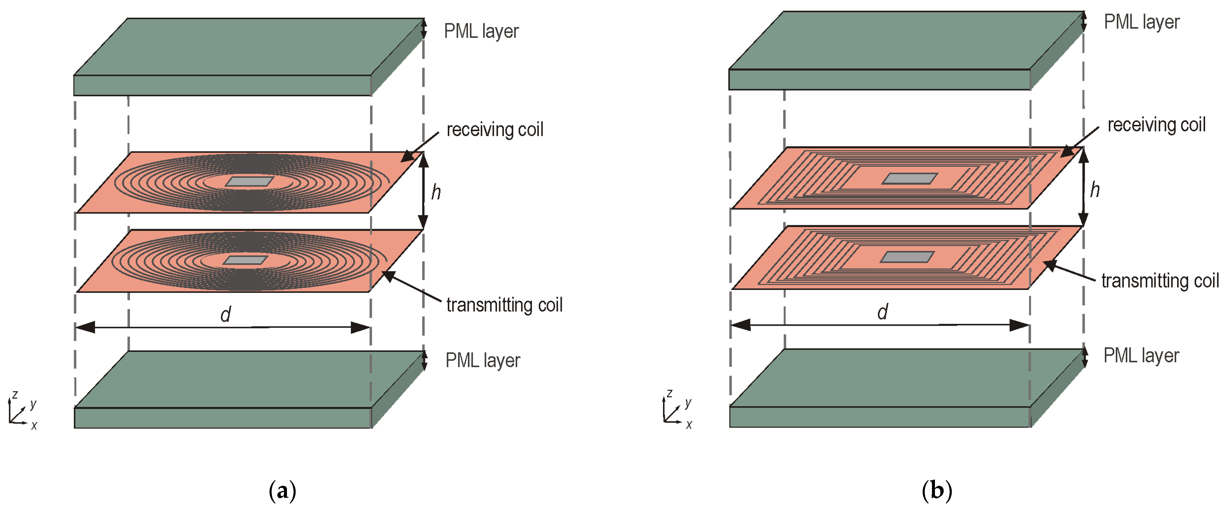
Figure 4.
The proposed numerical model of the single WPT cell with: (a) circular coils, (b) square coils.
Figure 4.
The proposed numerical model of the single WPT cell with: (a) circular coils, (b) square coils.
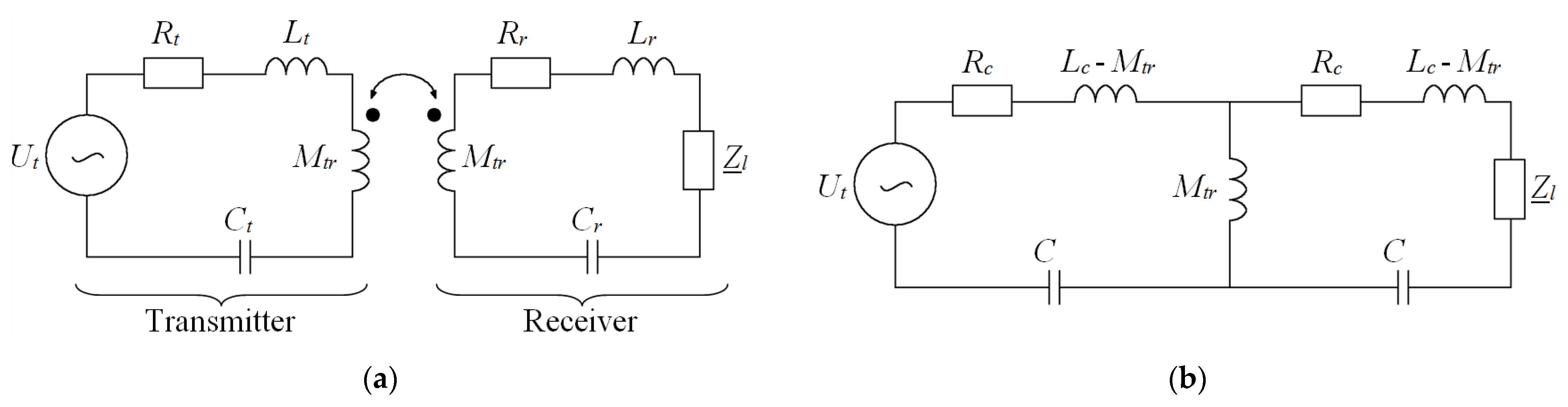
Figure 5.
Circuit model of the cell in the WPT system: (a) model with indicated magnetic coupling, (b) two-port network model of the cell with identical Tx and Rx coils.
Figure 5.
Circuit model of the cell in the WPT system: (a) model with indicated magnetic coupling, (b) two-port network model of the cell with identical Tx and Rx coils.
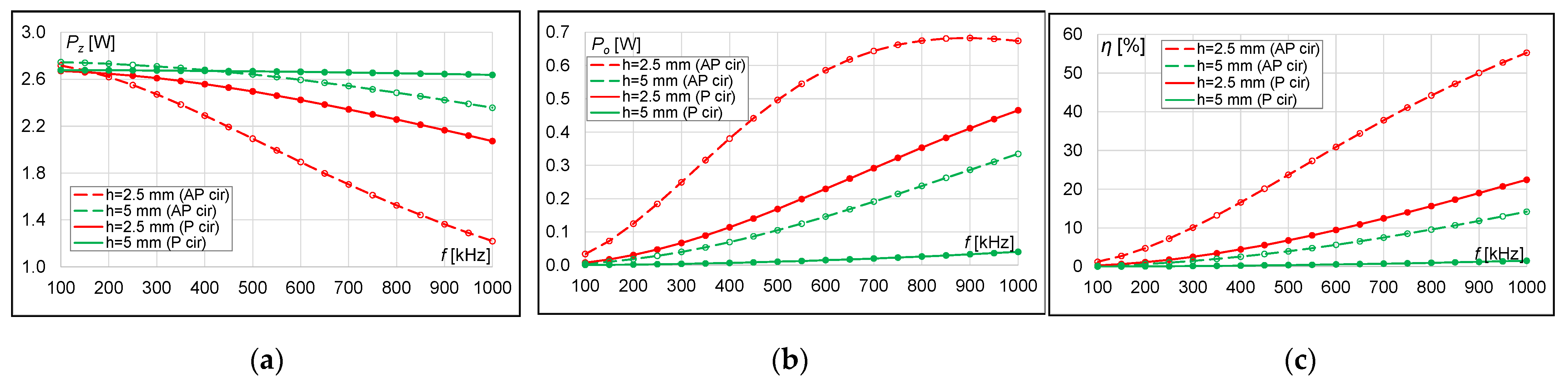
Figure 6.
Results for circular coils with r = 5 mm and the number of turns n = 15 at two distances (h = 2.5 mm and h = 5 mm): (a) transmitter power, (b) receiver power, (c) power transfer efficiency.
Figure 6.
Results for circular coils with r = 5 mm and the number of turns n = 15 at two distances (h = 2.5 mm and h = 5 mm): (a) transmitter power, (b) receiver power, (c) power transfer efficiency.
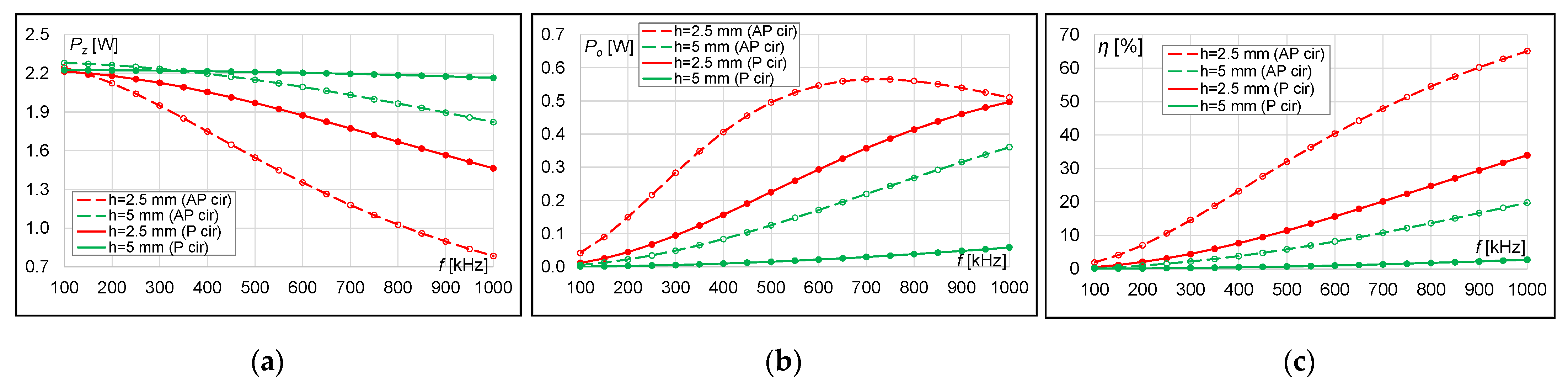
Figure 7.
Results for circular coils with r = 5 mm and the number of turns n = 20 at two distances (h = 2.5 mm and h = 5 mm): (a) transmitter power, (b) receiver power, (c) power transfer efficiency.
Figure 7.
Results for circular coils with r = 5 mm and the number of turns n = 20 at two distances (h = 2.5 mm and h = 5 mm): (a) transmitter power, (b) receiver power, (c) power transfer efficiency.
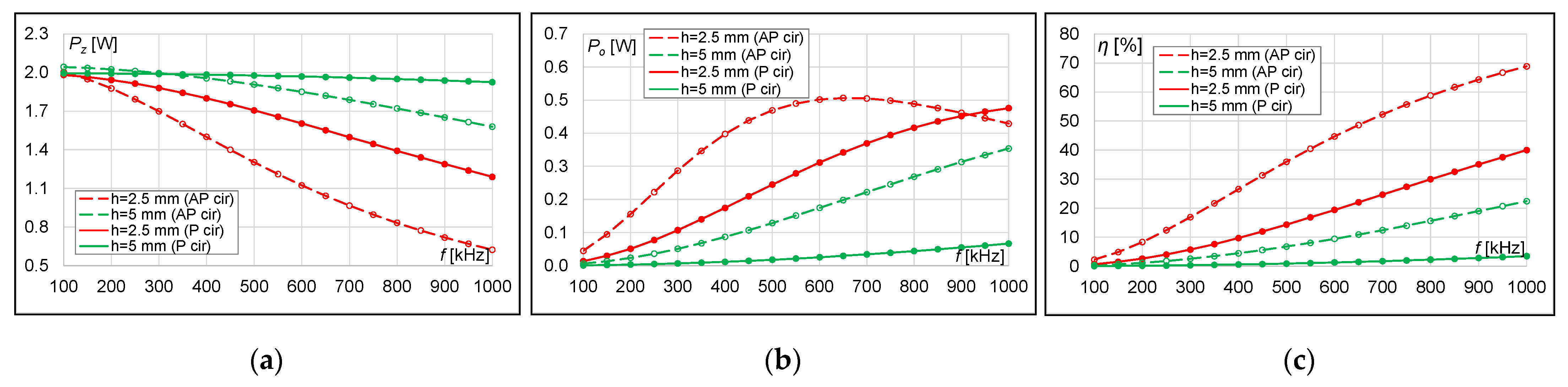
Figure 8.
Results for circular coils with r = 5 mm and the number of turns n = 25 at two distances (h = 2.5 mm and h = 5 mm): (a) transmitter power, (b) receiver power, (c) power transfer efficiency.
Figure 8.
Results for circular coils with r = 5 mm and the number of turns n = 25 at two distances (h = 2.5 mm and h = 5 mm): (a) transmitter power, (b) receiver power, (c) power transfer efficiency.
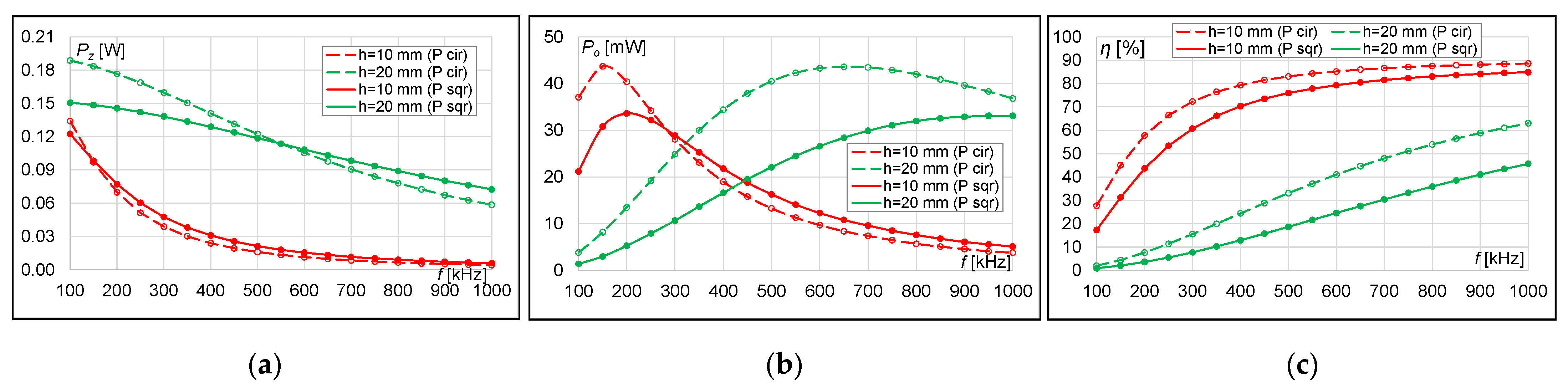
Figure 9.
Results for circular coils with r = 20 mm and the number of turns n = 40 at two distances (h = 10 mm and h = 20 mm): (a) transmitter power, (b) receiver power, (c) power transfer efficiency.
Figure 9.
Results for circular coils with r = 20 mm and the number of turns n = 40 at two distances (h = 10 mm and h = 20 mm): (a) transmitter power, (b) receiver power, (c) power transfer efficiency.
Figure 10.
Results for circular coils with r = 20 mm and the number of turns n = 50 at two distances (h = 10 mm and h = 20 mm): (a) transmitter power, (b) receiver power, (c) power transfer efficiency.
Figure 10.
Results for circular coils with r = 20 mm and the number of turns n = 50 at two distances (h = 10 mm and h = 20 mm): (a) transmitter power, (b) receiver power, (c) power transfer efficiency.
Figure 11.
Results for circular coils with r = 20 mm and the number of turns n = 60 at two distances (h = 10 mm and h = 20 mm): (a) transmitter power, (b) receiver power, (c) power transfer efficiency.
Figure 11.
Results for circular coils with r = 20 mm and the number of turns n = 60 at two distances (h = 10 mm and h = 20 mm): (a) transmitter power, (b) receiver power, (c) power transfer efficiency.
Figure 12.
Results for square coils with r = 5 mm and the number of turns n = 15 at two distances (h = 2.5 mm and h = 5 mm): (a) transmitter power, (b) receiver power, (c) power transfer efficiency.
Figure 12.
Results for square coils with r = 5 mm and the number of turns n = 15 at two distances (h = 2.5 mm and h = 5 mm): (a) transmitter power, (b) receiver power, (c) power transfer efficiency.
Figure 13.
Results for square coils with r = 5 mm and the number of turns n = 20 at two distances (h = 2.5 mm and h = 5 mm): (a) transmitter power, (b) receiver power, (c) power transfer efficiency.
Figure 13.
Results for square coils with r = 5 mm and the number of turns n = 20 at two distances (h = 2.5 mm and h = 5 mm): (a) transmitter power, (b) receiver power, (c) power transfer efficiency.
Figure 14.
Results for square coils with r = 5 mm and the number of turns n = 25 at two distances (h = 2.5 mm and h = 5 mm): (a) transmitter power, (b) receiver power, (c) power transfer efficiency.
Figure 14.
Results for square coils with r = 5 mm and the number of turns n = 25 at two distances (h = 2.5 mm and h = 5 mm): (a) transmitter power, (b) receiver power, (c) power transfer efficiency.
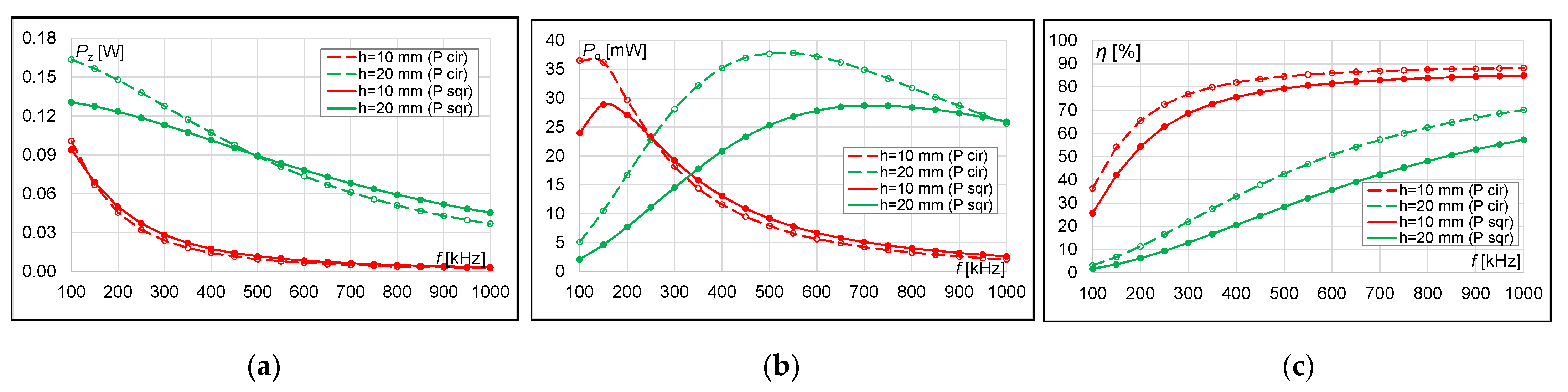
Figure 15.
Results for square coils with r = 20 mm and the number of turns n = 40 at two distances (h = 10 mm and h = 20 mm): (a) transmitter power, (b) receiver power, (c) power transfer efficiency.
Figure 15.
Results for square coils with r = 20 mm and the number of turns n = 40 at two distances (h = 10 mm and h = 20 mm): (a) transmitter power, (b) receiver power, (c) power transfer efficiency.
Figure 16.
Results for square coils with r = 20 mm and the number of turns n = 50 at two distances (h = 10 mm and h = 20 mm): (a) transmitter power, (b) receiver power, (c) power transfer efficiency.
Figure 16.
Results for square coils with r = 20 mm and the number of turns n = 50 at two distances (h = 10 mm and h = 20 mm): (a) transmitter power, (b) receiver power, (c) power transfer efficiency.
Figure 17.
Results for square coils with r = 20 mm and the number of turns n = 60 at two distances (h = 10 mm and h = 20 mm): (a) transmitter power, (b) receiver power, (c) power transfer efficiency.
Figure 17.
Results for square coils with r = 20 mm and the number of turns n = 60 at two distances (h = 10 mm and h = 20 mm): (a) transmitter power, (b) receiver power, (c) power transfer efficiency.
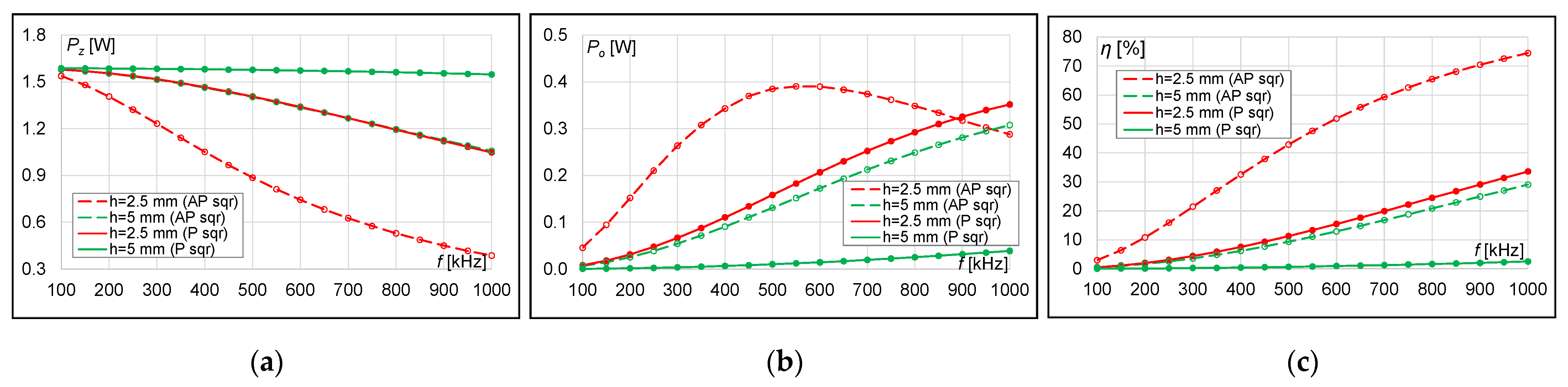
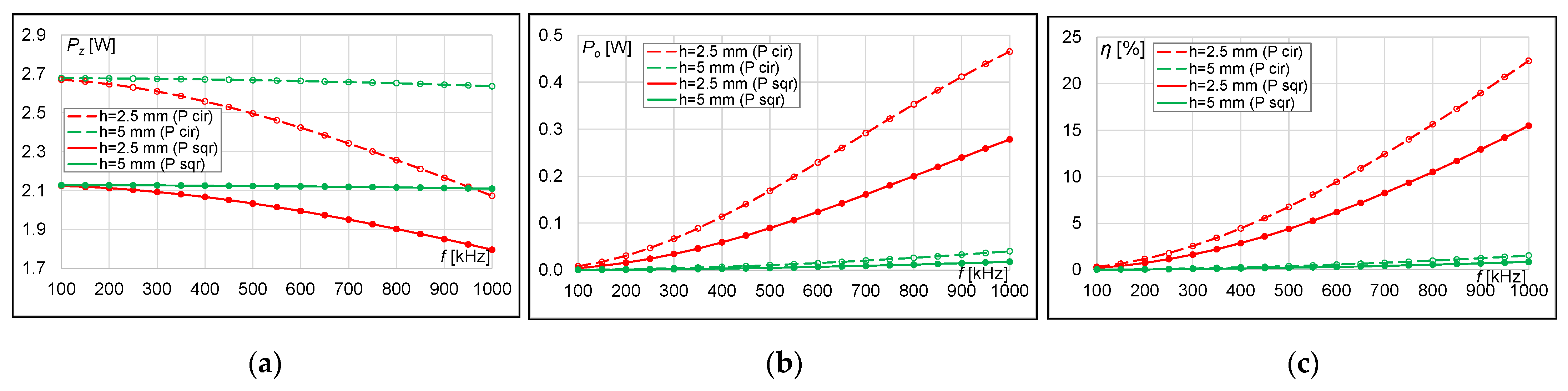
Figure 18.
Results for the periodic system with circular or square coils with r = 5 mm and the number of turns n = 15 at two distances (h = 2.5 mm and h = 5 mm): (a) transmitter power, (b) receiver power, (c) power transfer efficiency.
Figure 18.
Results for the periodic system with circular or square coils with r = 5 mm and the number of turns n = 15 at two distances (h = 2.5 mm and h = 5 mm): (a) transmitter power, (b) receiver power, (c) power transfer efficiency.
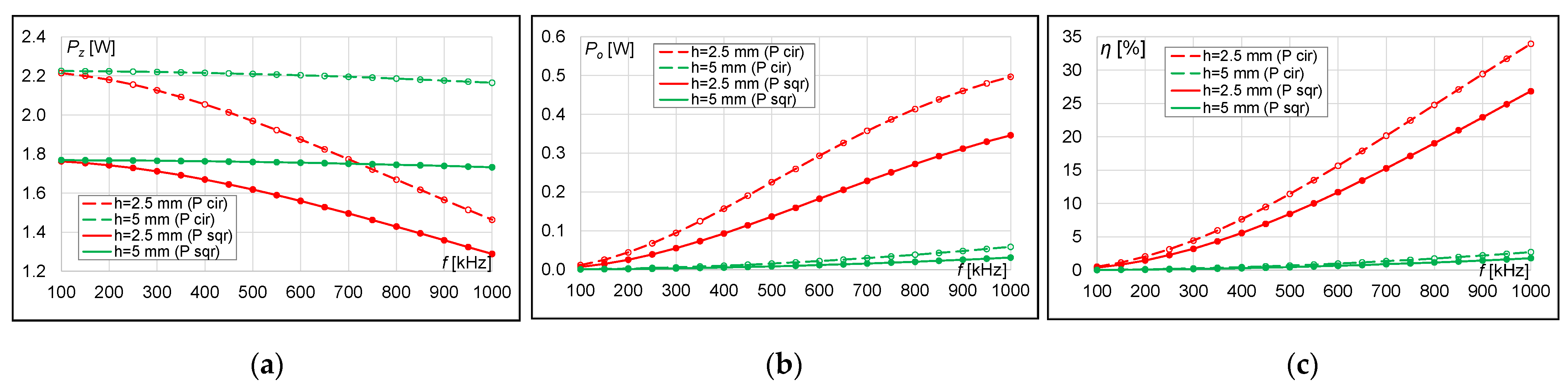
Figure 19.
Results for the periodic system with circular or square coils with r = 5 mm and the number of turns n = 20 at two distances (h = 2.5 mm and h = 5 mm): (a) transmitter power, (b) receiver power, (c) power transfer efficiency.
Figure 19.
Results for the periodic system with circular or square coils with r = 5 mm and the number of turns n = 20 at two distances (h = 2.5 mm and h = 5 mm): (a) transmitter power, (b) receiver power, (c) power transfer efficiency.
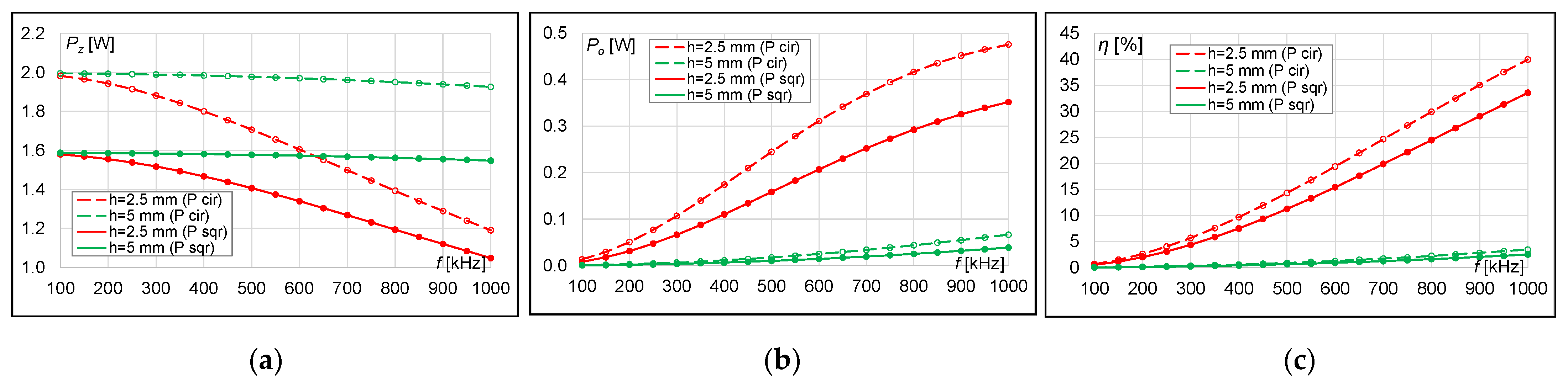
Figure 20.
Results for the periodic system with circular or square coils with r = 5 mm and the number of turns n = 25 at two distances (h = 2.5 mm and h = 5 mm): (a) transmitter power, (b) receiver power, (c) power transfer efficiency.
Figure 20.
Results for the periodic system with circular or square coils with r = 5 mm and the number of turns n = 25 at two distances (h = 2.5 mm and h = 5 mm): (a) transmitter power, (b) receiver power, (c) power transfer efficiency.
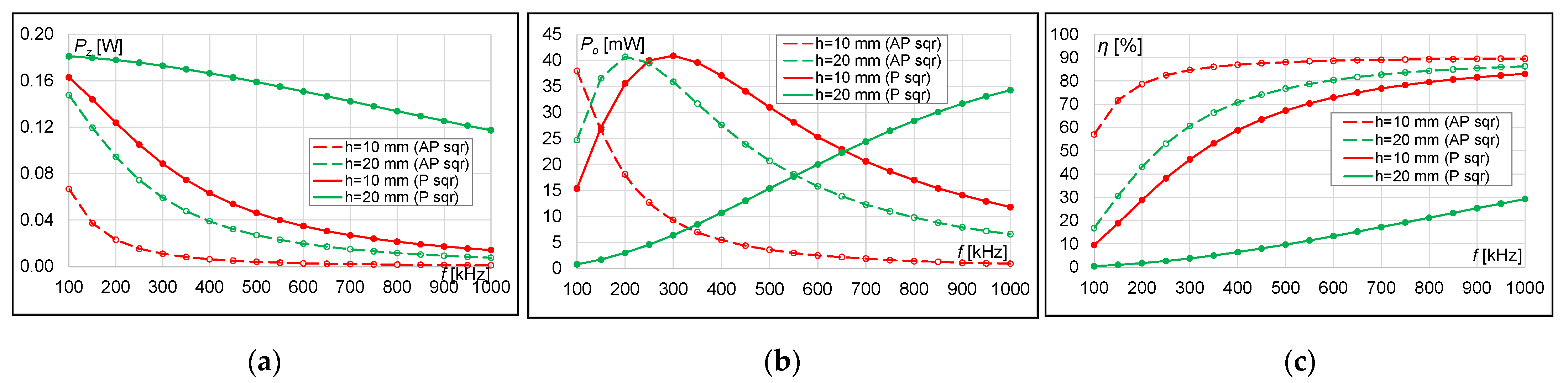
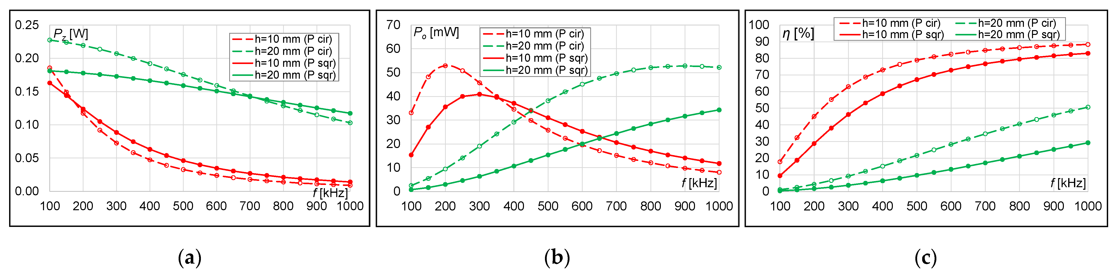
Figure 21.
Results for the periodic system with circular or square coils with r = 20 mm and the number of turns n = 40 at two distances (h = 10 mm and h = 20 mm): (a) transmitter power, (b) receiver power, (c) power transfer efficiency.
Figure 21.
Results for the periodic system with circular or square coils with r = 20 mm and the number of turns n = 40 at two distances (h = 10 mm and h = 20 mm): (a) transmitter power, (b) receiver power, (c) power transfer efficiency.
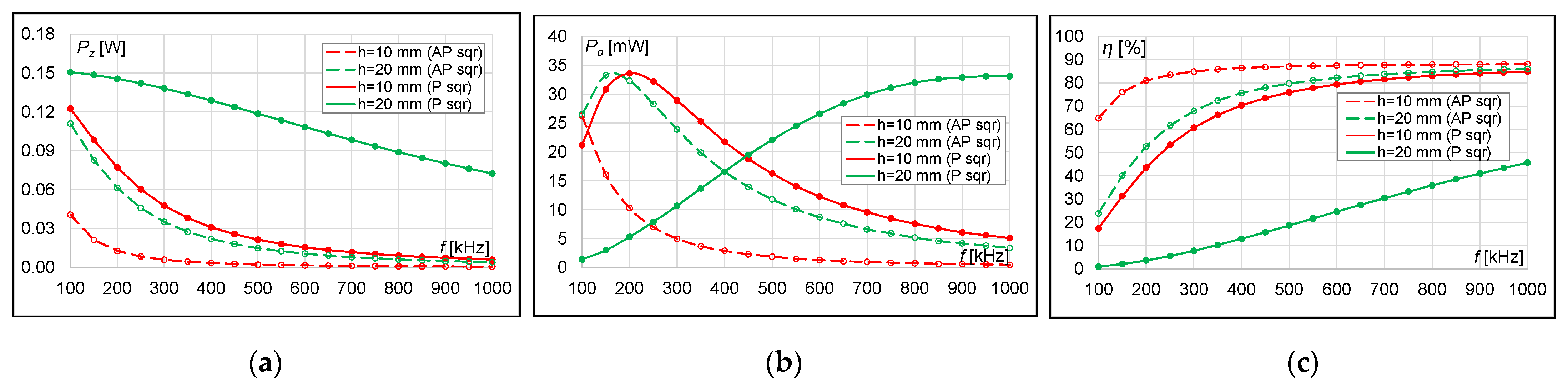
Figure 22.
Results for the periodic system with circular or square coils with r = 20 mm and the number of turns n = 50 at two distances (h = 10 mm and h = 20 mm): (a) transmitter power, (b) receiver power, (c) power transfer efficiency.
Figure 22.
Results for the periodic system with circular or square coils with r = 20 mm and the number of turns n = 50 at two distances (h = 10 mm and h = 20 mm): (a) transmitter power, (b) receiver power, (c) power transfer efficiency.
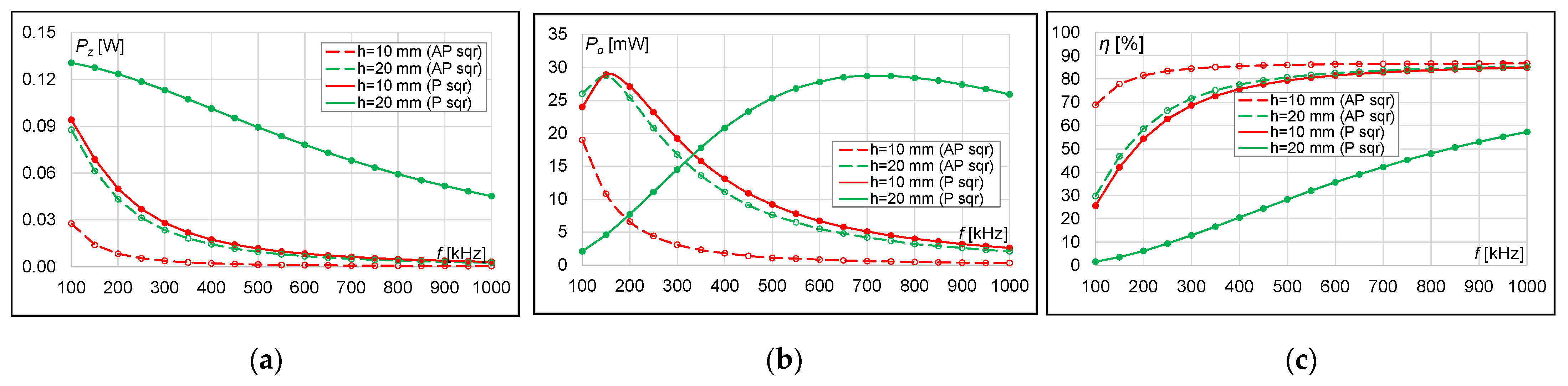
Figure 23.
Results for the periodic system with circular or square coils with r = 20 mm and the number of turns n = 60 at two distances (h = 10 mm and h = 20 mm): (a) transmitter power, (b) receiver power, (c) power transfer efficiency.
Figure 23.
Results for the periodic system with circular or square coils with r = 20 mm and the number of turns n = 60 at two distances (h = 10 mm and h = 20 mm): (a) transmitter power, (b) receiver power, (c) power transfer efficiency.
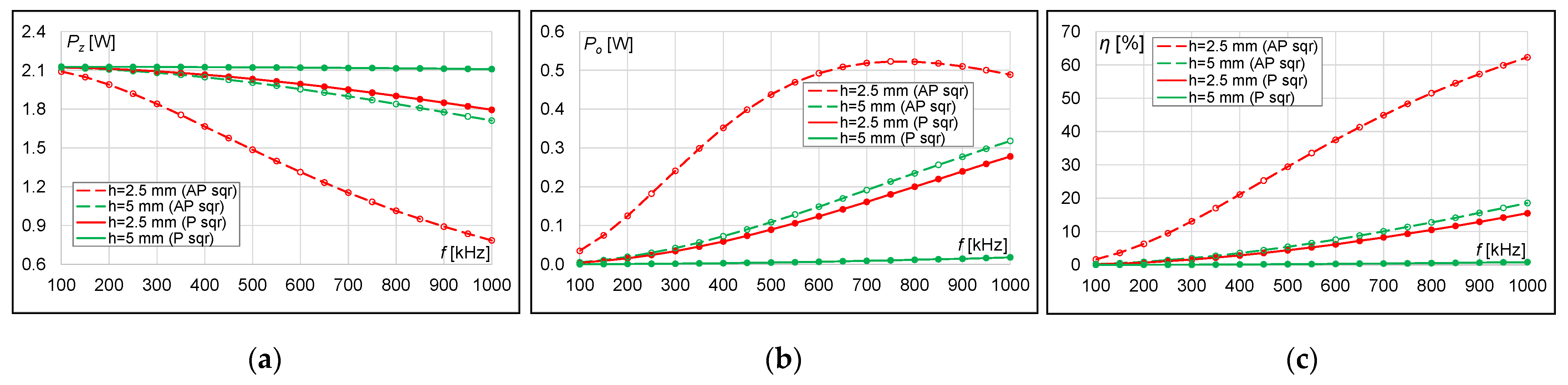
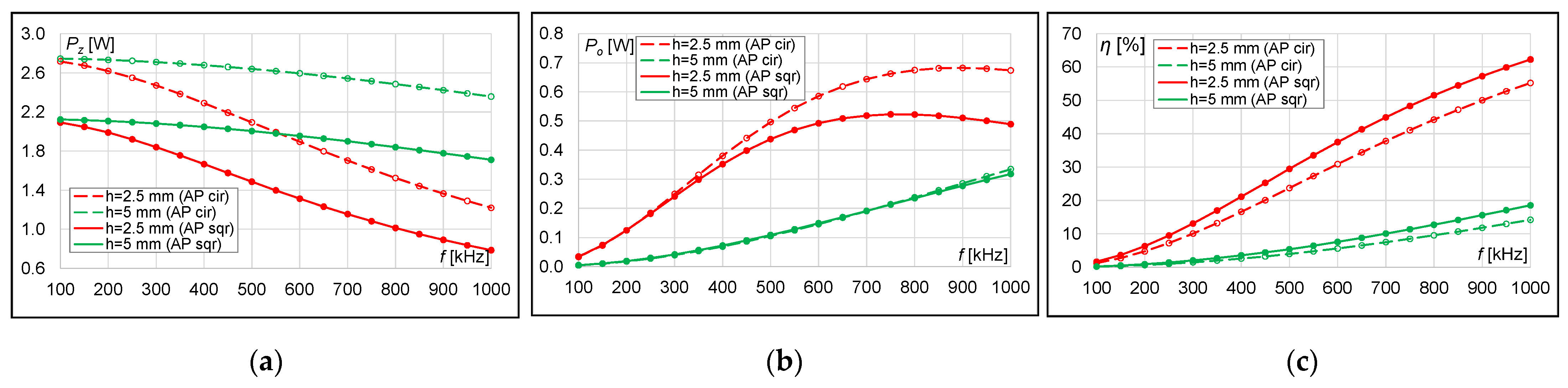
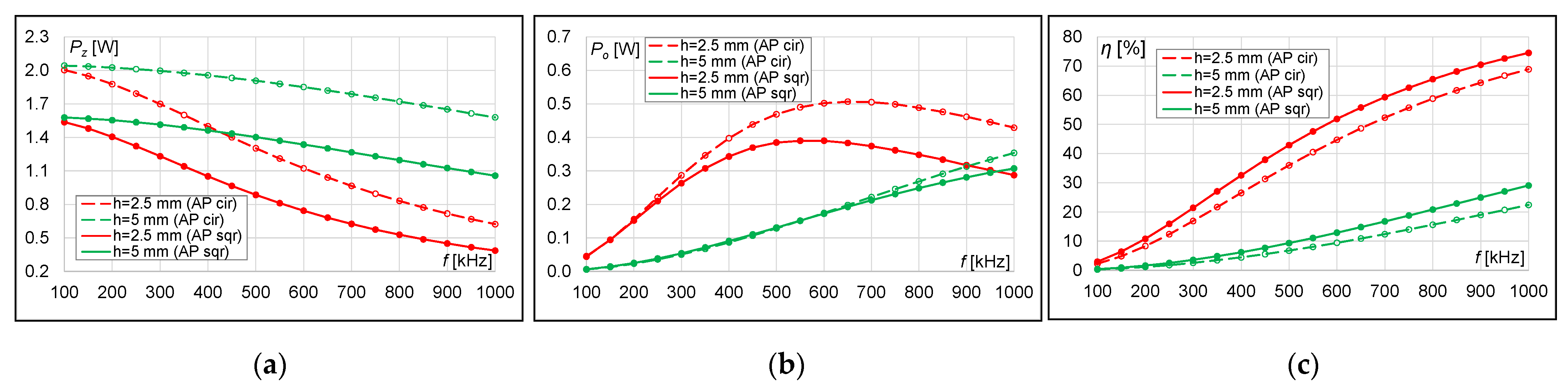
Figure 24.
Results for the aperiodic system with circular or square coils with r = 5 mm and the number of turns n = 15 at two distances (h = 2.5 mm and h = 5 mm): (a) transmitter power, (b) receiver power, (c) power transfer efficiency.
Figure 24.
Results for the aperiodic system with circular or square coils with r = 5 mm and the number of turns n = 15 at two distances (h = 2.5 mm and h = 5 mm): (a) transmitter power, (b) receiver power, (c) power transfer efficiency.
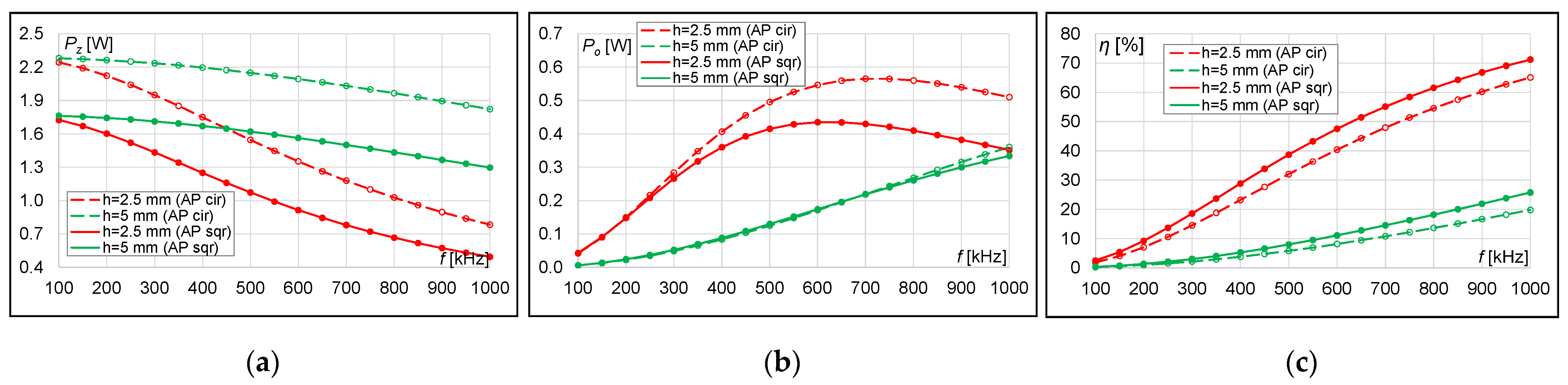
Figure 25.
Results for the aperiodic system with circular or square coils with r = 5 mm and the number of turns n = 20 at two distances (h = 2.5 mm and h = 5 mm): (a) transmitter power, (b) receiver power, (c) power transfer efficiency.
Figure 25.
Results for the aperiodic system with circular or square coils with r = 5 mm and the number of turns n = 20 at two distances (h = 2.5 mm and h = 5 mm): (a) transmitter power, (b) receiver power, (c) power transfer efficiency.
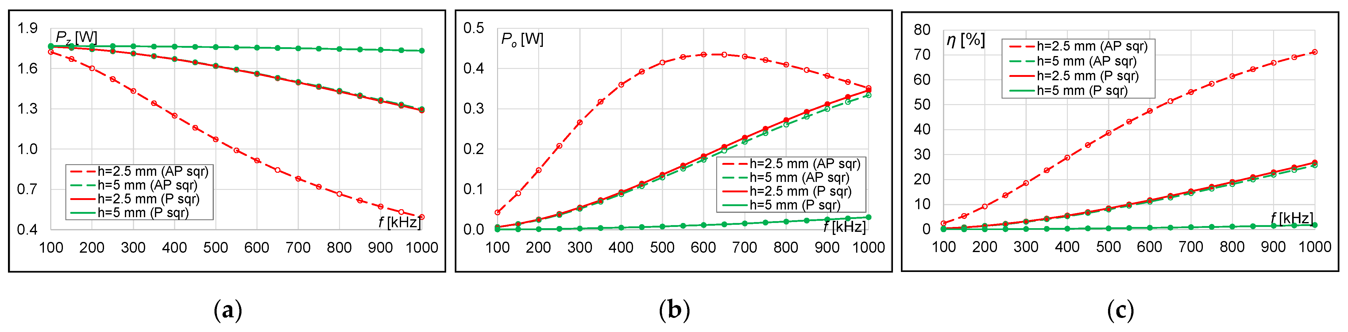
Figure 26.
Results for the aperiodic system with circular or square coils with r = 5 mm and the number of turns n = 25 at two distances (h = 2.5 mm and h = 5 mm): (a) transmitter power, (b) receiver power, (c) power transfer efficiency.
Figure 26.
Results for the aperiodic system with circular or square coils with r = 5 mm and the number of turns n = 25 at two distances (h = 2.5 mm and h = 5 mm): (a) transmitter power, (b) receiver power, (c) power transfer efficiency.
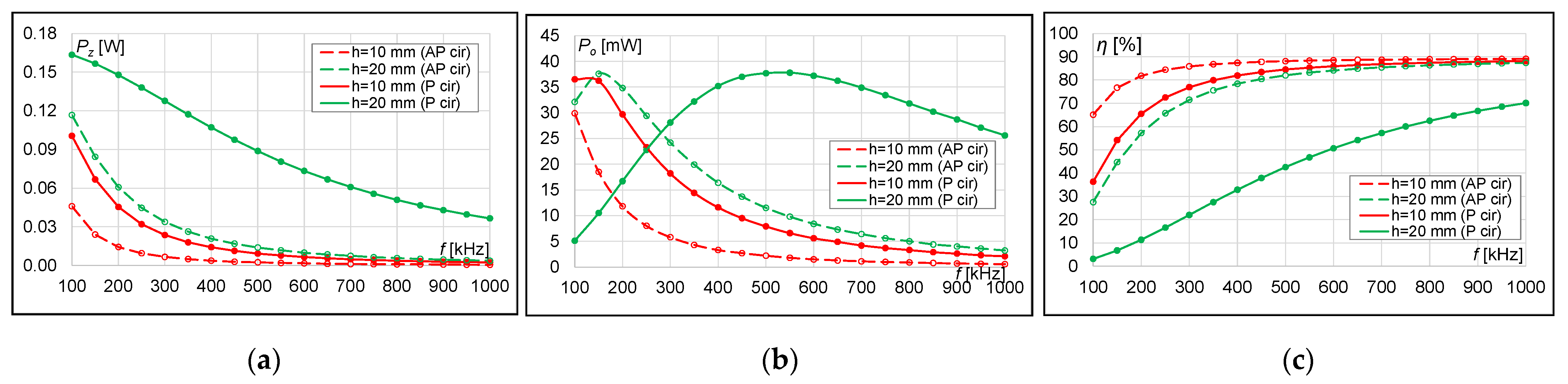
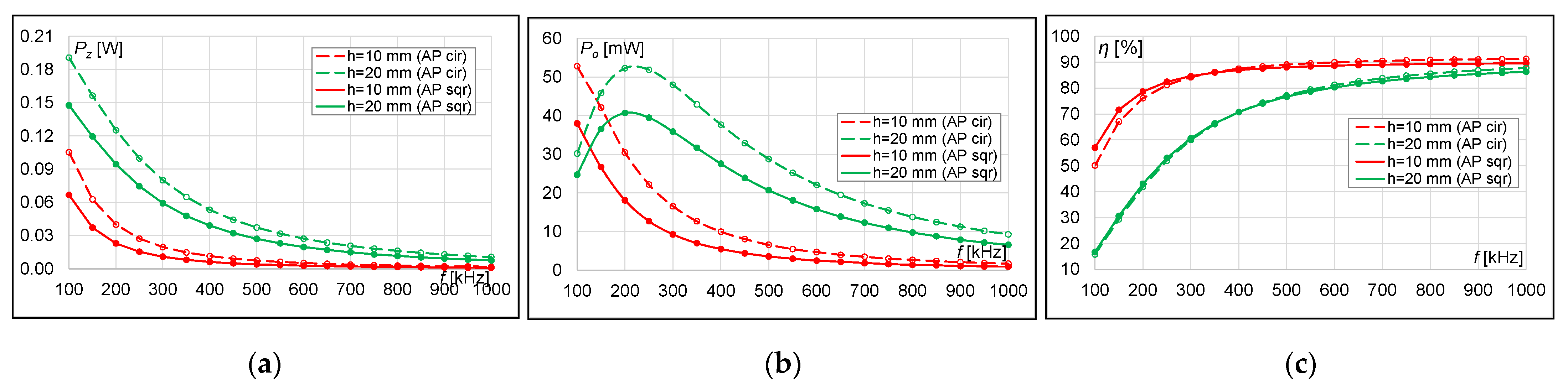
Figure 27.
Results for the aperiodic system with circular or square coils with r = 20 mm and the number of turns n = 40 at two distances (h = 10 mm and h = 20 mm): (a) transmitter power, (b) receiver power, (c) power transfer efficiency.
Figure 27.
Results for the aperiodic system with circular or square coils with r = 20 mm and the number of turns n = 40 at two distances (h = 10 mm and h = 20 mm): (a) transmitter power, (b) receiver power, (c) power transfer efficiency.
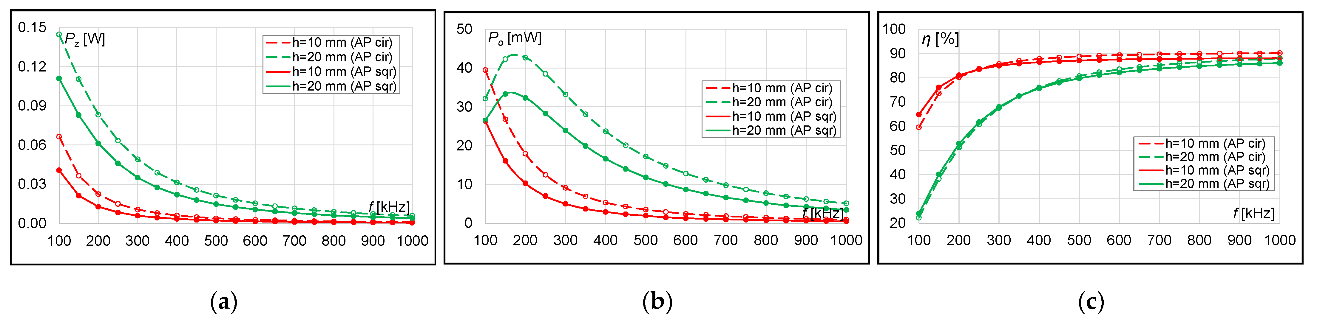
Figure 28.
Results for the aperiodic system with circular or square coils with r = 20 mm and the number of turns n = 50 at two distances (h = 10 mm and h = 20 mm): (a) transmitter power, (b) receiver power, (c) power transfer efficiency.
Figure 28.
Results for the aperiodic system with circular or square coils with r = 20 mm and the number of turns n = 50 at two distances (h = 10 mm and h = 20 mm): (a) transmitter power, (b) receiver power, (c) power transfer efficiency.
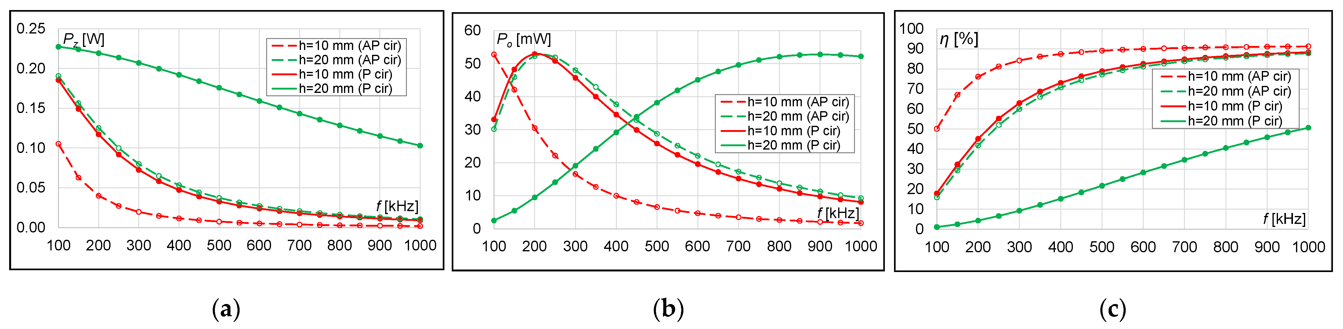
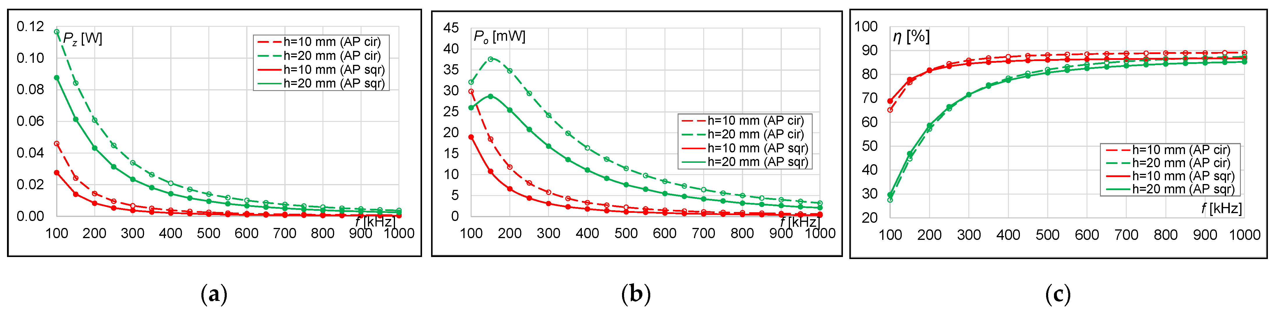
Figure 29.
Results for the aperiodic system with circular or square coils with r = 20 mm and the number of turns n = 60 at two distances (h = 10 mm and h = 20 mm): (a) transmitter power, (b) receiver power, (c) power transfer efficiency.
Figure 29.
Results for the aperiodic system with circular or square coils with r = 20 mm and the number of turns n = 60 at two distances (h = 10 mm and h = 20 mm): (a) transmitter power, (b) receiver power, (c) power transfer efficiency.
Table 1.
Parameters of the wire used to form the coils.
Table 1.
Parameters of the wire used to form the coils.
| Parameter | Symbol | Value |
|---|
| diameter of the wire | w | 150 µm |
| thickness of the wire insulation | i | 1 µm |
| conductivity of the wire | σ | 5.6·107 S/m |
| voltage source | Ut | 1 V |
| load impedance | Zl | 50 Ω |
| frequency domain | fmin ÷ fmax | 100 ÷ 1000 kHz |
Table 2.
Variants of geometric parameters taken for the analysis of two types of coils.
Table 2.
Variants of geometric parameters taken for the analysis of two types of coils.
| r (mm) | n | h (mm) |
|---|
| 0.5 r | r |
|---|
| 5 | 15 | 2.5 | 5.0 |
| 20 | 2.5 | 5.0 |
| 25 | 2.5 | 5.0 |
| 20 | 40 | 10.0 | 20.0 |
| 50 | 10.0 | 20.0 |
| 60 | 10.0 | 20.0 |
Table 3.
The values of the compensating capacity at fmax = 1 MHz, self, and mutual inductance for small circular and square coils (r = 5 mm).
Table 3.
The values of the compensating capacity at fmax = 1 MHz, self, and mutual inductance for small circular and square coils (r = 5 mm).
| n | Lself
(μH) | Mtr (nH) | C at fmax (nF) |
|---|
| Periodic | Aperiodic |
|---|
| h = 0.5 r | h = r | h = 0.5 r | h = r | Periodic | Aperiodic |
|---|
| Circular coils (r = 5 mm) |
| 15 | 2.36 | 373 | 86 | 784 | 286 | 13.26 | 10.72 |
| 20 | 3.14 | 547 | 127 | 1062 | 384 | 9.77 | 8.06 |
| 25 | 3.64 | 659 | 152 | 1227 | 439 | 8.30 | 6.95 |
| Square coils (r = 5 mm) |
| 15 | 3.09 | 334 | 72 | 1009 | 373 | 12.28 | 8.20 |
| 20 | 4.05 | 519 | 116 | 1365 | 505 | 9.03 | 6.25 |
| 25 | 4.64 | 645 | 145 | 1575 | 581 | 7.66 | 5.46 |
Table 4.
The values of the compensating capacity at fmax = 1 MHz, self, and mutual inductance for small circular and square coils (r = 20 mm).
Table 4.
The values of the compensating capacity at fmax = 1 MHz, self, and mutual inductance for small circular and square coils (r = 20 mm).
| n | Lself
(μH) | Mtr (μH) | C at fmax (pF) |
|---|
| Periodic | Aperiodic |
|---|
| h = 0.5 r | h = r | h = 0.5 r | h = r | Periodic | Aperiodic |
|---|
| Circular coils (r = 20 mm) |
| 40 | 91 | 12.00 | 2.72 | 28.57 | 10.46 | 348 | 280 |
| 50 | 122 | 17.85 | 4.09 | 39.66 | 14.50 | 258 | 208 |
| 60 | 151 | 23.89 | 5.51 | 50.20 | 18.30 | 207 | 167 |
| Square coils (r = 20 mm) |
| 40 | 120 | 9.52 | 1.93 | 36.47 | 13.29 | 329 | 211 |
| 50 | 160 | 15.14 | 3.17 | 50.76 | 18.65 | 242 | 158 |
| 60 | 198 | 21.36 | 4.60 | 64.55 | 23.84 | 192 | 128 |
Table 10.
The difference between the efficiency of the system in the periodic model and the aperiodic model with the use of circular coils.
Table 10.
The difference between the efficiency of the system in the periodic model and the aperiodic model with the use of circular coils.
| n | ∆η (%) at fmax |
|---|
| h = 0.5 r | h = r |
|---|
| for small coil (r = 5 mm) |
| 15 | 33% | 13% |
| 20 | 31% | 17% |
| 25 | 29% | 19% |
| for large coil (r = 20 mm) |
| 40 | 3% | 37% |
| 50 | 2% | 25% |
| 60 | 0.4% | 17% |
Table 11.
The difference between the efficiency of the system in the periodic model and the aperiodic model with the use of square coils.
Table 11.
The difference between the efficiency of the system in the periodic model and the aperiodic model with the use of square coils.
| n | ∆ η (%) at fmax |
|---|
| h = 0.5 r | h = r |
|---|
| for small coil (r = 5 mm) |
| 15 | 47% | 18% |
| 20 | 44% | 24% |
| 25 | 41% | 27% |
| for large coil (r = 20 mm) |
| 40 | 7% | 57% |
| 50 | 3% | 40% |
| 60 | 2% | 28% |
Table 12.
The difference between the efficiency of the system in the periodic models with circular or square coils.
Table 12.
The difference between the efficiency of the system in the periodic models with circular or square coils.
| n | ∆ η (%) at fmax |
|---|
| h = 0.5 r | h = r |
|---|
| for small coil (r = 5 mm) |
| 15 | 7% | 0.7% |
| 20 | 7% | 0.9% |
| 25 | 6% | 1% |
| for large coil (r = 20 mm) |
| 40 | 5% | 21% |
| 50 | 4% | 17% |
| 60 | 4% | 13% |
Table 13.
The difference between the efficiency of the system in the aperiodic models with circular or square coils.
Table 13.
The difference between the efficiency of the system in the aperiodic models with circular or square coils.
| n | ∆ η (%) at fmax |
|---|
| h = 0.5 r | h = r |
|---|
| for small coil (r = 5 mm) |
| 15 | 7% | 4% |
| 20 | 6% | 6% |
| 25 | 6% | 7% |
| for large coil (r = 20 mm) |
| 40 | 2% | 2% |
| 50 | 2% | 2% |
| 60 | 3% | 2% |


