1. Introduction
Recently, the use of renewable energy sources (RES) for reducing greenhouse gases and consequent sustainable development has been considered inevitable. The integration of RES has been successful to some extent, as various countries have actively implemented policies for wide integration, such as feed-in-tariffs and renewable portfolio standards, and the levelized cost of energy (LCOE) of RES has decreased through technological developments. The International Renewable Energy Agency (IRENA) reported that photovoltaic (PV) power generation tripled from 250 TWh in 2015 to 720 TWh in 2019 [
1]. Additionally, it was projected via an International Energy Agency (IEA) sustainable development scenario that approximately 3268 TWh will be produced by PV generation by 2030 [
2].
However, such an increase in PV generation causes instability in power systems due to its variability, intermittency, and limited controllability. Specifically, from the perspective of transmission system operators (TSOs), the unfavorable characteristics of RES, including PV generation, can exacerbate the imbalance between power supply and demand [
3] and make power system planning and operation more difficult [
4]. To address such problems, TSOs need to secure a significant number of flexible resources, which is then followed by an increase in the electricity bills of customers. Its threat to power systems is ongoing due to its unlimited access to the grid. For example, electricity consumption is frequently settled at a negative price in Germany, where 32.5% of gross power production is generated by wind and solar. The demand of the power system subtracted by generation of the RESs is called net demand, and their generation cannot be changed, much like usual demand, due to unlimited access to the grid. The reason for negative prices is that significantly reduced net demand, due to a surge in increased supply from RES at an instant, causes in the power system a condition of oversupply, requiring that inflexible generators with high ramp-up and ramp-down costs generate even for negative electricity prices. Therefore, a negative electricity price indicates a severe condition of a power system because its occurrence means the power system cannot remain in balance using only flexible resources [
5]. Furthermore, from the perspective of distribution system operators (DSOs), a high penetration of PV generation results in the need for investment in various alternative resources to achieve stable power system operation by addressing problems such as voltage fluctuation, increased network losses, and feeder overloading in the distribution network [
6,
7,
8].
Increasing the forecasting accuracy of PV generation is one of the most simple and economic solutions to such problems because it can incentivize balance-responsible parties (BRPs) in an attempt to reduce the penalty caused by the imbalance between the scheduled and actual PV generation. Ultra short-term forecasting is used in techniques such as power smoothing and real-time electricity dispatch. Short-term forecasting is useful for power scheduling tasks, such as unit commitment and economic power dispatch, and can also be used in PV-integrated energy management systems [
9]. In contrast, medium-term and long-term forecasting are effectively used in power system planning, where network optimization is performed and investment decisions are made [
10].
PV forecasting can be classified, according to its methodology, into physical methods, statistical approaches, and machine learning approaches [
9]. In physical methods, the radiant energy reaching the Earth’s surface is determined using a physical atmospheric model affecting the solar radiation. In Dolara et al. [
11], the PV output was forecasted using an irradiance model considering the transmittance of the atmosphere and an air-glass optical model. In statistical approaches, PV generation is forecasted through the statistical analysis of input variables. For instance, multi-period PV generation was forecasted using autoregressive moving average (ARMA) and autoregressive-integrated moving average (ARIMA) models in Colak et al. [
12], and an autoregressive moving average with exogenous inputs (ARMAX) model was applied to statistical PV forecasting by including weather forecasting data in Li et al. [
13]. In the last category of machine learning approaches, a forecasting model is trained by updating the model parameters based on existing data. Machine learning has wide applications, such as in dynamical systems with memory [
14] and health monitoring [
15]. Various machine learning models have been applied to forecasting PV generation, such as a support vector machine (SVM) [
16], Bayesian neural network [
17] and RNN-based models such as long short-term memory (LSTM) [
18] and gated recurrent network (GRU) [
19].
There have been attempts to separate the components of a forecasting target in the time series forecasting. In Keles et al. [
20], the spot prices in the electricity market were forecasted by separating them into deterministic and stochastic signals. In Zhu et al. [
21], Zang et al. [
22], and Li et al. [
23], time series data were decomposed using wavelet decomposition, and then the decomposed signals were used to teach a neural network. Similarly, time series data PV generation can be regarded as having seasonal and temporal components. The seasonal component results from changes in the altitude of the Sun due to the Earth’s orbit and rotation, while various stochastic factors, such as weather conditions, are the source of the temporal component.
On the other hand, there have been studies where PV generation data of similar dates during a year are combined to forecast the output. As the generations at similar dates have the seasonal component in common, their combination leads to more accurate forecasting of the seasonal component. Thus, a forecasting method using the seasonal component is likely to show a good forecasting performance. PV generation data of adjacent days were used in the convolution neural network (CNN) [
22] and the time correlation method [
24]. In Li et al. [
25], the seasonal component was forecast using the weighted sum of the two outputs from the CNN with inputs of PV generation at adjacent days and from the LSTM with inputs of total PV generation over one day. The forecasting error can be reduced by indirectly considering seasonal changes through the regularizing effect of an ensemble model. In Wen et al. [
26], the ensemble of a back-propagation neural network, radial basis function neural network, extreme learning machine, and Elman neural network was used for forecasting the seasonal component of PV generation, and in Gigoni et al. [
27], the combination of the Grey-box model, neural nework, k-nearest neighbor, quantile random forest, and support vector regression was the best in terms of forecasting accuracy.
Table 1 summarizes prior studies on PV generation forecasting by method.
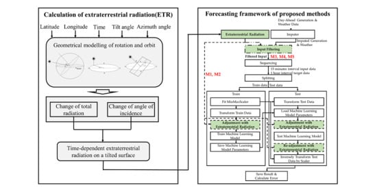
In contrast to the approaches used in the previous studies, the seasonal component can be determined more accurately by direct geometric modeling, based on the fact that solar radiation changes periodically according to the Earth’s rotation and orbit. Thus, in this study, we propose methods to calculate the seasonal component using the angle of incidence and solar constant for improving forecasting accuracy, and those methods are verified using four different neural network models: MLP and three RNN-based models including Vanilla RNN, LSTM, and GRU. The contribution of this paper is as follows.
This is the first study that explicitly introduces extraterrestrial radiation, that is, the solar radiation outside the atmosphere, into various neural network models;
Methods for integrating the extraterrestrial radiation into neural network models for PV generating forecasting are presented;
To verify the effectiveness of the proposed methods, the methods are applied to four neural network models: MLP and three RNN-based models including Vanilla RNN, LSTM, and GRU. Then, their forecasting performances are examined and compared.
2. Seasonal Changes in Extraterrestrial Radiation
Extraterrestrial radiation (ETR) refers to the power per unit area of sunlight irradiated at the distance between the Sun and the Earth in space. The ETR is radiation that does not consider the effects of the atmosphere and acts as an upper limit of the energy from the Sun reaching the Earth. The ETR has a seasonal characteristic because the Earth’s orbit and rotation are seasonal. The parameters for modeling the seasonality of the ETR include the change in the distance between the Sun and Earth, the change in the solar declination due to the Earth’s orbit, and the circumferential motion of the Sun due to the Earth’s rotation.
Since the Earth’s orbit is not circular but elliptical, the distance between the Sun and the Earth changes according to the orbit, which causes corresponding changes in radiation. In addition, since the Earth orbits the Sun with its rotation axis tilted by 23.5 degrees, the declination of the Sun varies with time, which is associated with the amount of sunlight throughout the year. The Earth’s rotation also affects the radiation throughout the day, that is, there is a large amount of radiation during the day in contrast to the absence of radiation during the night.
In this study, the ETR was geometrically determined as a function of time based on the diurnal motion model. Specifically, the solar constant was used to determine the maximum of daily ETR, and then it was adjusted according to the angle of incidence of the Sun with respect to the PV panel.
2.1. Solar Constant
The solar constant,
, is defined as the power per unit area irradiated from the Sun at the average distance between the Sun and Earth. It can be measured from a satellite to eliminate the atmospheric effect and determined as [
28]:
The radiation on a surface perpendicular to the sunlight on the
-th day of a year, denoted as
, is calculated as [
29]:
2.2. Angle of Incidence
The ETR parallel to the final radiation incident on the PV panel is obtained considering the angle of incidence (θ), which means the angle between the radiation and the orthogonal line to the PV panel. The angle of incidence can be derived as a function of time by geometric modeling. The necessary variables include not only the declination, hour angle, latitude, and longitude but also the tilt angle and azimuth angle, which are the angles defining the geometric configuration of the PV panels.
2.2.1. Declination
As illustrated in
Figure 1, the declination (
) is defined as the angle between the lines connecting the Sun and the Equator in the equatorial coordinate system. It has a positive value in the Northern Hemisphere. The declination on the
-th day of a year can be approximately determined as [
28]:
2.2.2. Hour Angle
The Sun’s position in the celestial coordinate system can be expressed as a function of time within a day by considering the circumferential motion of the Sun due to the Earth’s rotation. However, to accurately integrate the time zone into the geometrical model, the local time needs to be converted into solar time, which is determined based on the Sun, following the rule as follows [
28]:
where
and
are the longitudes of Local Standard Time Meridian and the longitude at a specific location, respectively, and
is calculated as:
Then, the solar time is further converted into the hour angle (
) according to the following relationship as:
The hour angle is conceptually illustrated in
Figure 2.
2.2.3. Tilt and Azimuth of PV Panels
The PV panels are installed with a slope to maximize the amount of power generated by minimizing the angle of incidence. The parameters defining the geometrical configuration of a PV panel consist of tilt (
β) and azimuth (
γ), which are shown in
Figure 3. The tilt is the angle between the horizontal plane and the PV panel. The azimuth is the angle measured from the Meridian to the point where the normal vector of the PV panel is projected orthogonal to the horizontal plane, and thus it is positive in the western area and negative in the eastern area [
28].
2.2.4. Calculation of the Angle of Incidence
2.3. Calculation of the Extraterrestrial Radiation
Once the solar constant and the angle of incidence at a place of interest are calculated according to (2) and (8), the value of ETR, denoted as
, can be simply calculated as:
For instance, the process of calculating the ETR was applied to a place in Yulara, Australia. The resulting values of the ETR for a tilted surface on the first day of each month throughout a year are shown in
Figure 4. The values of ETR had the same bell shape as a typical clear-sky PV generation over a day. The place is located in the Southern Hemisphere and, thus, the Sun’s altitude and the corresponding value of
are the highest in December and January. Accordingly, the ETR is the greatest in those months. The final radiance on the PV panel had the same bell-shaped pattern, but with more fluctuations depending on weather conditions. Consequently, the ETR can be interpreted as a piece of clean information on radiation by the Sun with noise from the atmosphere removed.
3. Forecasting Models
In this section, the traditional persistent model and representative neural network models are briefly described, which are used for comparison purposes in the case study later.
3.1. Persistence Model
In the persistence model, PV outputs of yesterday are used as forecasted PV generation. Although the persistence model is simple, it shows a satisfactory forecasting performance, particularly when the weather conditions do not change significantly. The persistence model was used as a reference in a study comparing the forecasting accuracy.
3.2. Multilayer Perceptron
The multilayer perceptron (MLP) is a model where nodes that imitate a human neural network are stacked in series and parallel. The node receives input data, multiplies them by its weights, applies its activation function to the intermediate value, and finally generates the outputs. The wider and deeper the nodes are, the more complex the functions can be modeled.
A learning process is performed by computing the gradient of the loss function and updating the weights of a node using the back-propagation algorithm. If the MLP is deep with many layers, a vanishing gradient problem can occur, which means the gradient is no longer passed to the previous layers. Some activation functions, such as the rectified linear unit (ReLU), can mitigate the vanishing gradient problem. The MLP can be regarded as more effective and flexible than traditional regression models because there is no assumption on the form of the target function to be modeled.
3.3. Recurrent Neural Network
Unlike the MLP, the recurrent neural network (RNN) has a memory function that is implemented by sequentially feeding back the outputs or states in the previous times to the current input. Obviously, the outputs in the previous times contain the information in the past. This property makes the RNN suitable for dealing with time series data. The learning process of the RNN is performed by the technique of back-propagation through time, which unfolds the RNN with respect to time and applies the same back-propagation algorithm as the MLP. However, the weights of the RNN have the risk of divergence, particularly when handling a long sequence of data, because the same weight parameters are updated repetitively during training.
To address the divergence problem, gate structures are proposed for the RNN, called gated RNN, such as long short-term memory (LSTM) and gated recurrent unit (GRU). The gates in the gated RNN determine which information is retained or discarded in the hidden state. Nodes constituting the gates make these decisions. The nodes applies the sigmoid function as their activation function to their intermediate outputs, which are then multiplied with the hidden state. As the sigmoid function is bounded in (0, 1), only a portion of the hidden states is preserved by multiplication, meaning the gate considers the portion important. The parameters of the nodes are added to those of the simple RNN, and they are also updated in the learning process so that the gates make effective decisions. It has been empirically verified that gated RNNs have better characteristics in terms of convergence and accuracy for the forecasting task of a long sequence. Recently, gated RNNs have been widely used for time series forecasting [
29,
30].
3.3.1. Vanilla RNN
Vanilla RNN is a preliminary RNN structure that stores historic information by a hidden state. The hidden state at time
(
) is determined by applying the hyperbolic tangent function to the weighted sum of the current input and hidden states in the previous times as follows:
where
are the weights;
is the bias;
is the input at time
t; and
is the output at time
t. 3.3.2. Long Short-Term Memory
Figure 5 shows the structure of a cell in the LSTM. The cell has the input, forget, and output gates that determine the output through weight update Equations in (11)–(14).
where
are the weights;
are the biases;
and
are the input and output at time
;
,
, and
are the input, forget, and output gates at time
, respectively;
is the candidate;
is the sigmoid function. The function of the three gates of the LSTM cell is implemented as the element-wise multiplication, denoted as
x around a circle in
Figure 6. Specifically, the forget gate eliminates unnecessary information from the cell state (
) in the previous time; the input gate extracts important information from the input; the output gate generates the selective output from the sigmoid function values (
) for the hidden state (
) in the previous time.
3.3.3. Gated Recurrent Unit
Unlike the LSTM, the cell of the GRU has two gates, that is, a reset gate and an update gate (
Figure 6). The update equations associated with the gates are given as:
where
are the weights;
are the biases;
and
are the input and output at time
;
and
are the update and reset gates at time
, respectively;
is the candidate;
denotes the Hadamard product; and
is the sigmoid function. The functions of the reset and update gates of the GRU are similar to those of the forget and input gates of the LSTM. Therefore, there is no significant difference between the structures of the GRU and LSTM. However, the number of weights of the GRU are fewer than that of the LSTM, which results in higher efficiency in the learning process of the GRU.
5. Case Study
5.1. Dataset
In the case study, datasets provided by the Desert Knowledge Australia Solar Centre (DKASC) in Australia were used [
31,
32]. DKASC operates solar power plants in Alice Springs and Yulara in Australia, and their information is listed in
Table 2.
The datasets provided by DKASC contain both meteorological information and PV power generation data in the two regions. The specific features in the dataset are listed in
Table 3. The feature of wind direction was excluded because it increased the forecasting error. The features of global horizontal radiation and diffuse horizontal radiation were not chosen either, because it strongly correlates with PV generation [
9]. Pyranometer measurement was also excluded, as it measures radiation in a specific frequency band.
The total period of data used in the case study was from May 2016 to January 2021. Among them, the data from May 2016 to January 2020 were used for training; the remaining data over the year from February 2020 to January 2021 were used for the test.
5.2. Models and Performance Index
The effectiveness of the proposed methods was verified and compared using four representative neural network models: MLP, Vanilla RNN, LSTM, and GRU.
To evaluate the forecasting performance, two types of indexes, that is, mean squared error (
MSE) and mean absolute error (
MAE), were used. The two indexes are defined as follows:
where
is the number of samples,
is the predictors,
is the target output, and
is the output forecasted by a model. To determine the hyperparameters of the models, 10-fold cross-validation was conducted by randomly sampling 10 subsets with equal size from the training set and using each of the subsets for validation in each stage of validation. The resulting hyperparameters of the models are listed in
Table 4. The Adam optimizer was used in the training. Epoch was determined as 150 because the average of 10-fold validation errors were saturated and oscillated in a small range after being trained 60~90 times, and increased after being trained over 200 times, as shown in
Figure 9.
Figure 9 also shows the average of a 10-fold training error of the same model, which steadily declined as the epoch increased. This means the model had enough capacity to fit the training data, validating a reasonable choice of the size of the hidden states. The difference in scale between the validation error and training error was because MinMaxScaler was applied during training. Learning rate schedulers were not used in this study, because they can make the model converge into a poor local minimum, which leads to a higher
MSE. The RNN-based models were configured to be bidirectional, as shown in
Figure 10, because it is more effective to consider future data and predicted outputs for prediction especially for the day-ahead forecasting. A simple two-layer MLP model was applied to the output of the RNN-based models to reduce the dimension of the hidden states to one.
5.3. Results
The proposed methods were applied to the four neural network models described in
Section 5.2 for the two datasets. The results are listed in
Table 5 and
Table 6. Each method was trained and tested 20 times for each combination of the model and the dataset to examine its effect on average.
As a result, M5 was the most effective in the majority of the dataset-model combinations.
Table 7 shows the improvements M5 achieved relative to the base method in RNN-based models. M5 reduced the MSE by 4.1% on average and, at most, by 12.28% in the RNN-based models. These results imply that integrating ETR into neural network models can improve model performance without additional investment in data collection. The fact that M5 had consistently higher performance than other methods under different datasets and RNN-based models means that M5 can be expected to be effective when one forecasts PV generation without verifying which method would be the best.
We analyzed the results of each method, from which important lessons were derived as follows. First, for M1, two points are notable: (1) Comparing the performance of M1 with the persistence model on each dataset to consider the relative error, the performance on the BP Solar dataset was worse than that on the Desert Gardens dataset. (2) Even though M5 was superior most of the time, the performance of M1 was the best when MLP was used on the BP Solar dataset. From point (1), it can be derived that the performance of each method varies considerably between different datasets even though they are not vastly different, as their geographical locations are similar. From point (2), it can be derived that the performance of each method varies across different models. The reason that M1 featured a large error in one of the datasets is inferred as follows. When normalized, PV generation in timeslots with small ETR and large ETR become closer to each other. Then, gradient signals with similar magnitudes are backpropagated in each timeslot during training, the two timeslots being treated equally even though their ETRs are different. During testing, the outputs of the model are multiplied by ETR, which leads to amplification of the error. If trained inappropriately, forecasting in the timeslots with a large ETR can be inaccurate compared with a small ETR, resulting in a higher MSE than the base method. However, as shown in point (2), M1 can be the best method depending on the forecasting configuration. Therefore, rather than using the best method for a different dataset, it is important to verify the competitiveness of each method by validation to choose the best method for the dataset and model used. M2 had better performance than M1 on average. Nevertheless, it is not certainly superior to the base method, implying that adjusting the gradient signal can affect the result inappropriately.
M3, which replaces the historical generation with ETR, performed poorly in general. In particular, the MSE of M3 was higher by 150% than the base method when the Desert Gardens dataset and RNN-based models were used. This result suggests two implications: (1) Assuming that ETR performed as a good baseline for prediction, inaccurate forecasting of M3 means a lack of enough meteorological data to predict the attenuation ratio of the atmosphere. (2) Comparing the situations with and without day-ahead generation, the superior performance of the method that includes day-ahead generation implies that day-ahead PV forecasting is effective by using day-ahead generation as a baseline for the prediction. In other words, the neural network-based models improve their performance from the persistence model by considering meteorological information.
The results of M4 and M5 can be analyzed from the perspective above. M4 and M5, which take day-ahead PV generation as one of the inputs, had additional improvement by having one more feature than the base method with day-ahead generation as a baseline. M4 including raw ETR as one of the inputs saw decent improvement in the Desert Gardens dataset while performing worse in the BP Solar dataset. It was more desirable to adjust ETR using meteorological information most of the time in this experiment.
Although M5 had a general advantage in our experiments, there are various circumstances in which PV generation is forecasted in a day-ahead manner in real world applications, and the effectiveness of each method varies depending on models and datasets. Therefore, it should be noted that for a given model and dataset, various methods should be evaluated by validation to effectively integrate ETR into a forecasting model.
6. Conclusions
This study presents a simple and effective method to improve the forecasting accuracy of PV generation for mitigating the problems caused by the inherent characteristics of PV, such as variability, intermittency, and limited controllability. This study focused on the ETR strongly associated with the seasonal component of PV as a means to improve forecasting performance. We selected neural network models as the basic forecasting method. Then, we composed five methods to integrate the ETR into them and examined the effect in terms of forecasting performance. The specific integration methods were (1) division preprocessing, (2) multiplication preprocessing, (3) replacement of existing input, (4) inclusion as additional input, and (5) inclusion as an intermediate target.
The methods were tested on MLP, Vanilla RNN, LSTM, and GRU using the two PV datasets. The results show that combining the ETR with existing models can achieve meaningful improvement in forecasting performance and present a new approach to considering seasonal changes in PV generation. Among the methods, including the ETR as an intermediate target (i.e., M5) showed relatively better results than the other integration methods. However, the combination of M5 with Vanilla RNN was the best for one dataset, but the combination of M5 with LSTM was the best for the other. Thus, a certain neural network model combined with the ETR did not show absolute superiority as usual with the comparison results between AI methods.
This study was limited to a few selected neural network models, even though they are known as the methods that effectively deal with time series data. Thus, the effectiveness of the proposed integration methods of the ETR can be further examined in other neural network models. It is also necessary that the proposed methods be applied to other PV datasets in extended studies. Then, the relative superiority of M5 can be further evaluated and more elaborate advice for combining the ETR with neural network-based models can be given.


