Article

Hybrid Energy Routing Approach for Energy Internet

1
LRSD Laboratory, Computer Science Department, Ferhat ABBAS Sétif 1 University, 19000 Sétif, Algeria
2
College of Information Technology, United Arab Emirates University, Al Ain 15551, United Arab Emirates
3
Smart ICT Laboratory, National School of Applied Sciences, Mohammed First University, 60000 Oujda, Morocco
*
Author to whom correspondence should be addressed.
Energies 2021, 14(9), 2579; https://doi.org/10.3390/en14092579
Submission received: 29 March 2021 / Revised: 23 April 2021 / Accepted: 26 April 2021 / Published: 30 April 2021

Abstract

:
The Energy Internet (EI) has been proposed as an evolution of the power system in order to improve its efficiency in terms of energy generation, transmission and consumption. It aims to make the use of renewable energy effective. Herein, the energy router has been considered the crucial element that builds the net structure between the different EI components by connecting and controlling the bidirectional power and data flow. The increased use of renewable energy sources in EI has contributed to the creation of a new competitive energy trading market known as peer-to-peer energy trading, which enables each component to be part of the trading process. As a consequence, the concept of energy routing is increasingly relevant. In fact, there are three issues that need to be taken into account during the energy routing process: the subscriber matching, the energy-efficient path and the transmission scheduling. In this work, we first proposed a peer-to-peer energy trading scheme to ensure a controllable and reliable EI. Then, we introduced a new energy routing approach to address the three routing issues. A subscriber matching mechanism is designed to determine which producer/producers should be assigned for each consumer by optimizing the energy cost and transmission losses. This mechanism provides a solution for both mono and multi-source consumers. An improved ant colony optimization-based energy routing protocol was developed to determine a non-congestion minimum loss path. For the multi-source consumer case, an energy particle swarm optimization algorithm was proposed to choose a set of producers and to decide the amount of energy that should be collected from each producer to satisfy the consumer request. Finally, the performance of the proposed protocol, in terms of power losses, cost and computation time was compared to the best existing algorithms in the literature. Simulation results show the effectiveness of the proposed approach.

1. Introduction

Due to the increase in energy demand and price, the environmental pollution resulting from conventional energy production techniques based on fossil fuel (coil, crud oil and natural gas), the development of environmentally friendly energy known as renewable energy, such as solar, wind and tide, has become necessary and attracted a lot of attention. The integration of renewable energy in the energy system reduces the CO 2 emissions, the transmission costs of energy and the load placed on the main grid by supplying a percentage of the demand through local energy production and consumption. Transforming energy production from conventional techniques to fully rely on renewable energy sources in the energy network cannot completely guarantee energy self-balancing due to its dispersion, discontinuity and volatility properties. The generation of energy, by these renewable sources, depends on weather conditions. Thus, renewable energy sources must be connected with the utility grid and controlled using sensing capabilities with information and communication technologies which creates smart grids [1]. According to National Institute of Standards and Technology (NIST), USA, the smart grid (SG) is: “A modernized grid that enables bidirectional flows of energy and uses two-way communication and control capabilities that will lead to an array of new functionalities and applications”. While SG uses an intelligent and digitized network, some restrictions still remain. In the aim of developing and completing the issues of smart grids, the EI was proposed [2,3]. The concept of EI, also called the Internet of energy and future smart grid, was proposed for the first time by the American economist Jeremy Rifkin in his book “The Third Industrial Revolution: How Lateral Power Is Transforming Energy, the Economy, and the World” [4], to solve the problems of existing energy systems. Jeremy Rifkin defined the EI as an energy system combined with the Internet technology in the aim of making an effective use of renewable energy, increasing the energy efficiency and the reliability of the electrical power system. EI is a complex energy system in which different energy networks are connected, such as: power grids, cooling/heating systems, natural gas networks, distributed energy generation, storage systems and loads [3]. The principle of EI is based on the integration of Internet technology, renewable energy, advanced technologies such as smart monitoring, intelligent management and large data processing with the existing energy systems [5,6]. The main objective of EI is to create a sustainable energy system with high energy efficiency, significant cost saving, minimum power losses and the high improvement of the use of distributed renewable energy sources (DREs).
As we mentioned before, the EI supports several forms of energy. In this paper, the energy flow is stored and distributed in the form of electrical energy.
In the conventional electrical power system, the power flow is unidirectional, generated by large scale power plant, transmitted to substations via high-voltage transmission lines and distributed to end users through low-voltage distribution lines. Accordingly, the power market is often structured in a unidirectional form, where generation companies generally sell huge amounts of electric energy to wholesale retailers, while retailers sell the electric energy to end users in smaller amounts [7,8]. With the concept of feed-in-tariffs (FiTs) in SG, consumers equipped with distributed renewable energy sources (DREs) referred to as prosumers—they can generate and consume electricity—are able to directly contribute in the power market by selling their excess energy to the utility grid (company) [9]. Many studies have been proposed in this regard to insure the supply–demand balance in the SG and to maximize the profit of the power market. Authors in [10] proposed a Stackelberg game-theoretic approach between the utility company and various prosumers, in which the utility company acts as a leader and announces an energy price, while the prosumers act as followers and adjust their electricity consumption according to the announced price. However, the authors in [11] proposed a contract-theoritic demand response management approach that aims to maximize the profit of both utility grid and prosumers in the SG. Unfortunately, the benefit of the involved prosumers in the FiT systems has been limited, prompting researchers to determine other trading schemes to encourage prosumers to become involved in power trading [12]. In contrast, EI is a peer-to-peer energy sharing system with a bidirectional flow of power and communication. The emergence of P2P distributed energy trading (sharing) in EI provides a new public energy market with new features in the power system. It enables prosumers to trade and share their excess energy (power) with each other directly in peer-to-peer mode without the interaction of a central entity such as a utility company [13]. This peer-to-peer mode of energy exchange gives energy producers and consumers the opportunity to create some financial benefits by selling the excess energy (generally with a lower cost than the cost of a utility company) instead of storing it for future use, which creates some power losses. Additionally, it decreases the consumer’s electricity bills and the reliance on the main grid (utility company). As far as we know, due to its complex technologies and infrastructures, there is no standardized architectural model for P2P electrical energy trading and various types of P2P distributed energy trading architectures have been designed by various studies [14,15,16,17].
The expansion of the use of DREs in power generation with their volatility, the transformation of the generation and the injection of power from centralized to distributed manner, the peer-to-peer energy sharing and the power losses during the energy transmission process make the distribution of energy and the balancing of energy supply/demand in EI more difficult. All of these variables gave rise to the key issue of the Energy Internet, which is the energy routing issue. It is known that there is some power losses during energy transmission process between producers and consumers. In order to minimize the power losses and to create efficient energy delivery over the EI, energy routing has been suggested which was inspired by data routing on the Internet. Energy routing is the process that facilitates the transmission of energy between prosumers and consumers situated in different geographic locations with the minimum power transmission losses. The key element of EI and energy routing is the energy router (ER), which is used to route both information and energy flow [18,19]. Current energy systems do not have this capability. However, energy routing in distributed energy systems is more complicated due to integration problems; because power conversion from one type to another may be needed. Energy routing has received considerable attention from the research community in recent years. Current research on this issue includes designing energy routing devices and energy routing algorithms. A number of researchers considered energy routing as data routing and therefore suggested devices and protocols for energy routing. Nonetheless, energy routing criteria are distinct from data routing (see Table 1). The waste packet can be resent in the Internet, which is not possible in EI. In addition, energy routing is demand-driven and the source of the energy is not defined [13]. Furthermore, an energy overflow may cause system devices or even the whole system to crash. Therefore, energy routing has more requirements on safety and reliability than data routing. For that, energy routing protocols are the main field of research for working on EI. These energy routing algorithms need to solve three main problems: the subscriber matching problem by determining the best producer for each consumer; the efficient energy routing problem by selecting the best path with the minimum power loss between these producer–consumer pairs; and finally, scheduling these energy transmissions to prevent congestion or overflow problems.
Current literature indicates that the different energy routing algorithms proposed to solve the energy routing are usually based on graph theory, game theory, mixed integer programming and autonomous systems. In the graph theory-based routing algorithms, the grid is presented as a graph and routing methods are applied to find the lowest cost path such as: the protocol proposed by Wang et all in paper [20]. In this work, the proposed energy routing protocol finds all the possible paths between the consumer and producer in the grid, and then determines the best path among them. This solution is not practical, especially in large grids, as the proposed protocol assumes that the transmission capacity of transmission lines is large enough. In paper [21], the authors proposed a distributed routing algorithm based on Dijkstra algorithm. This study did not investigate how the prosumer–consumer pairs are created. The authors in [22] proposed a hierarchical energy routing protocol where a master node determines all efficient paths between each pair in the grid, which affects the security and efficiency of the grid, and could cause the one point failure of the system. However, game theory has been widely used in power systems to solve different issues such as the demand response optimization problem including the work in [23] where a Stackelberg game approach was proposed in order to reduce the peak load and balance the supply–demand in the smart grid. The proposed approach determines the efficient consumption scheduling for consumers based on the real-time pricing. The authors in [24] used the reinforcement learning with the game theory and proposed an approach to solve the demand response problem in SG—in which a reinforcement learning mechanism was used to determine the best company for each consumer based on the electricity price and availability, and game theory based-demand response management technique to schedule the consumer consumption. Several game theory based-approaches [25,26,27,28] have been proposed to solve the energy routing problem in the peer-to-peer energy trading market. In these approaches, producers and consumers play a game (such us Stackelberg game, Coalition game … etc.) to create the producer/prosumer–consumer pairs with the maximization of their benefits. An energy routing algorithm based on an autonomous system is proposed in [29] where each system entity acts as an agent in the trading process. Authors in [30] proposed an energy trading platform with a mixed integer programming model for the optimal sharing energy between different houses in the EI in order to create a total profit for all participant houses. This work introduced a decision-making process that allows houses to determine when they should buy or sell energy, but it did not investigate the efficient path and scheduling problems. However, the authors in [31] suggested the use of bio-inspired methods to solve the energy routing problem. They considered the energy routing problem as an optimization problem and proposed the use of Ant Colony Optimization (ACO) to solve it. The proposed protocol calculates the minimum loss path between producers and consumers using the distance with the average cost by mile. A distributed Bee Colony Optimization (BCO)-based energy routing protocol is proposed in [32] to determine the best producer for each consumer considering the power loss, distance and available power among producers. The authors in [33] proposed an optimized energy routing method using Particle Swarm Optimization (PSO). It determined the energy-efficient path between producers and consumers in the SG by considering the links’ quality, transmission cost and latency in the selection of the best optimal neighbors. There are other considerations than distance to be included in the estimation of the power loss, which will be addressed in detail in the next section. Based on the previous analysis, we considered in this paper the energy routing problem with its surrounding issues (subscriber matching, efficient path and transmission scheduling) as an optimization problem. To solve this problem, we proposed an improvement of the existing energy routing method in [31]. The contributions of this paper are:
  • A peer-to-peer energy trading architecture based on energy routers;
  • A subscriber matching mechanism, and an Energy Particle Swarm Optimization Algorithm (EPSOA). The proposed subscriber matching mechanism determines the consumer–producer pairs for both mono and multi-source consumer cases (normal and heavy loads). The EPSOA is used in a heavy load case to determine the amount power to buy from a set of producers to insure minimum power transmission loss and cost;
  • An Improved energy routing protocol based on ant colony optimization which calculates a non-congestion minimum loss path between each producer/consumer pair in the EI.
The remaining sections of the paper are organized as follows. Section 2 describes the proposed EI based on energy routers. It is modeled as a weighted graph. Section 3 introduces the subscriber matching mechanism, the energy particle swarm optimization method with the centralized peer-to-peer energy trading network. The Improved Ant Colony Optimization (IACO)-based energy routing protocol is detailed in Section 4. The performance of the proposed algorithms is evaluated by various analysis cases. It is also compared to the algorithm described in Section 5 in terms of power losses, costs and computation time. Finally, Section 7 concludes the paper.

2. Implementation of Energy Internet with Energy Routers

In this section, the structure of ER-based energy Internet and its graph theory representation are introduced. The concept and functions of ER are discussed.

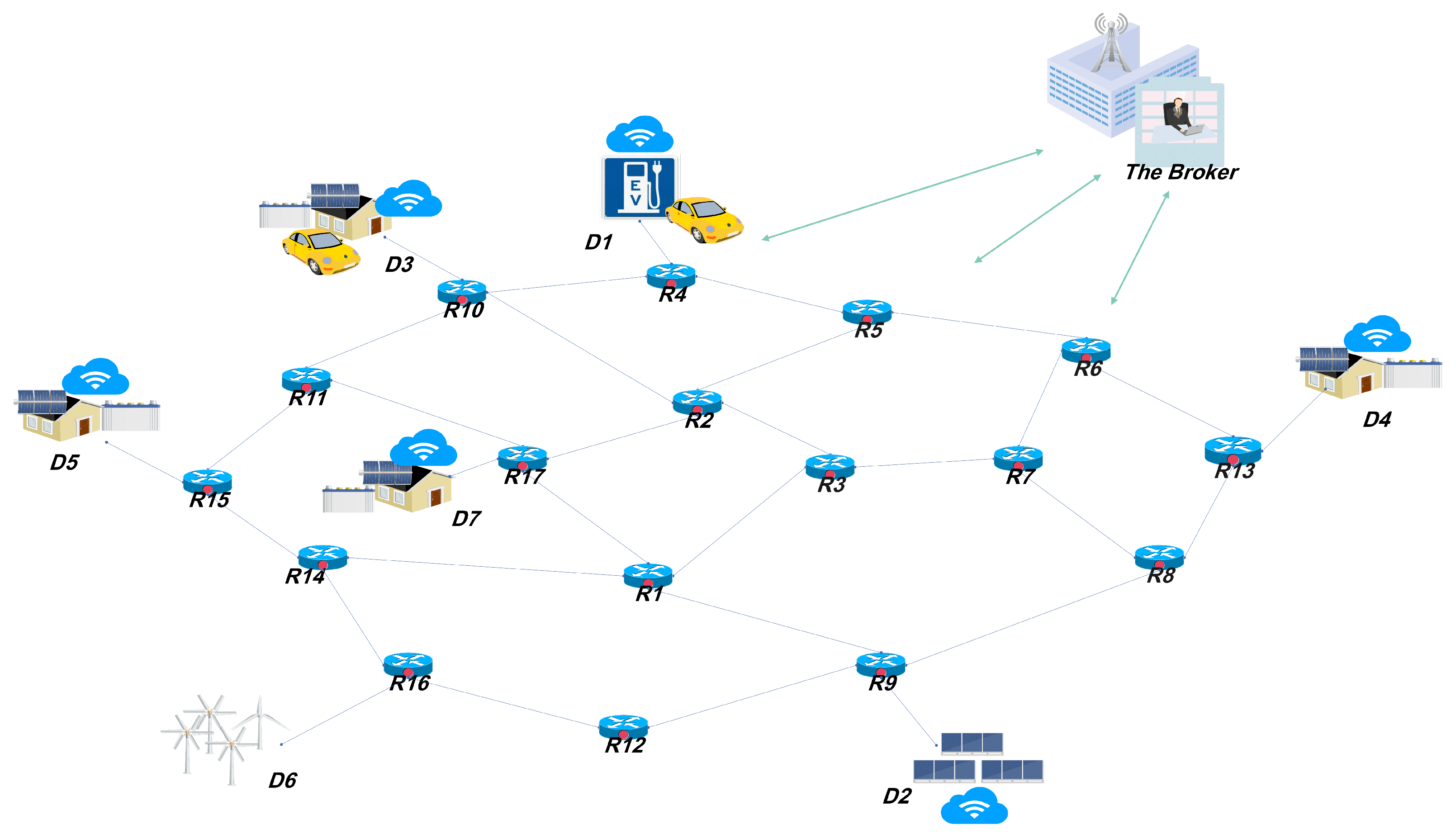
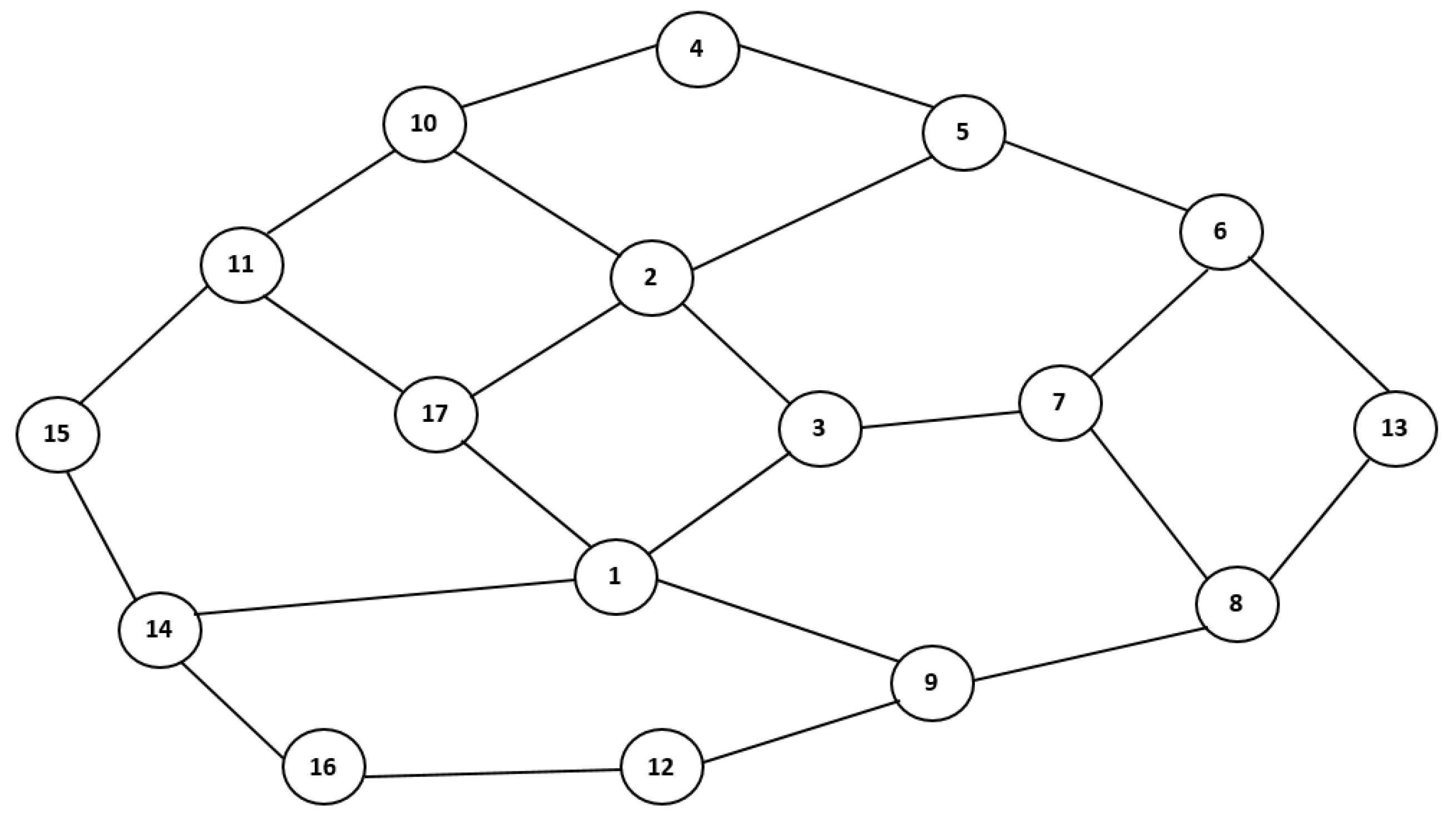
2.1. Structure of Energy Internet with Energy Routers:

As illustrated in Figure 1, the proposed energy router-based EI in this paper consists of different passive consumers (e.g., smart homes, industrial users, buildings, EVs), distributed power generation units such as solar and wind power, distributed energy storage units, and active consumers referred to as prosumers. As mentioned earlier, a prosumer is a consumer equipped with DREs (such as solar panels, wind turbines) to generate and consume electricity. In this work, the prosumer is represented by a smart home equipped with solar panels, such as in [34]. In the SG, prosumers trade their surplus energy with the utility grid for a small feed-in-tariff rate, which is not the only trading option in the EI. As mentioned earlier, the EI is a peer-to-peer energy sharing system that enables passive consumers equipped with distributed energy sources to trade directly and share energy with each other without the interaction of the utility grid. This creates some benefits for prosumers, consumers and the utility grid. All these elements are connected to a net structure using power lines and energy routers.
In our system, we consider that the grid used is a three-phase electrical grid characterized by the composed voltage V = 400 v, and the frequency of 50 Hz. The apparent power requested by the consumer is:
S A p p a r e n t = P 2 + Q 2
where P represents the active power ( P = 3 × V × I × c o s ( ϕ ) ) and Q is the reactive power ( Q = 3 × V × I × s i n ( ϕ ) ) with I , c o s ( ϕ ) represents the line current and the power factor, respectively. In general c o s ( ϕ ) > 0.95 , and as a result, the reactive power becomes negligible, and the apparent power is approximately equal to the active power ( S A p p a r e n t P ). The producer produces power that is an active power since the energy router (converters) do not inject reactive power into the grid.
In the aim of creating an efficient, scheduled, stable and controlled peer-to-peer energy trading market, we propose a centralized peer-to-peer energy trading architecture that contains a principal actor, named the broker. This broker manages the energy market and adjusts to balance the supply and demand in the energy system by satisfying consumers requests without the need of adding new energy generation units. The broker’s role will be discussed in detail in the following section.
Using graph theory, the proposed EI is modeled as a weighted graph G = { V , E , W } as shown in Figure 2.
  • Energy routers are represented by a set of vertices V = { v 1 , v 2 , , v n } ;
  • Power lines used for connecting energy routers are represented by a set of edges E = { e ij , } , where e ij is the power line that connects router v i to router v j ;
  • W describes the adjacency matrix of the network W = ( w ij ) n × n , which reflects the network topology with the weights of both ERs and power lines of EI as shown in Equation (2).
    w ij = w e ij e ij E w v i i = j e ij E
    where w e ij is the weight of the edge e ij , which represents the power loss of the power line that connects routers v i and v j . While w v i is the weight of ER v i , which represents its power loss. Both weights of power lines and energy routers are determined by Equations (15), (18) and (19) as shown in Section 5.

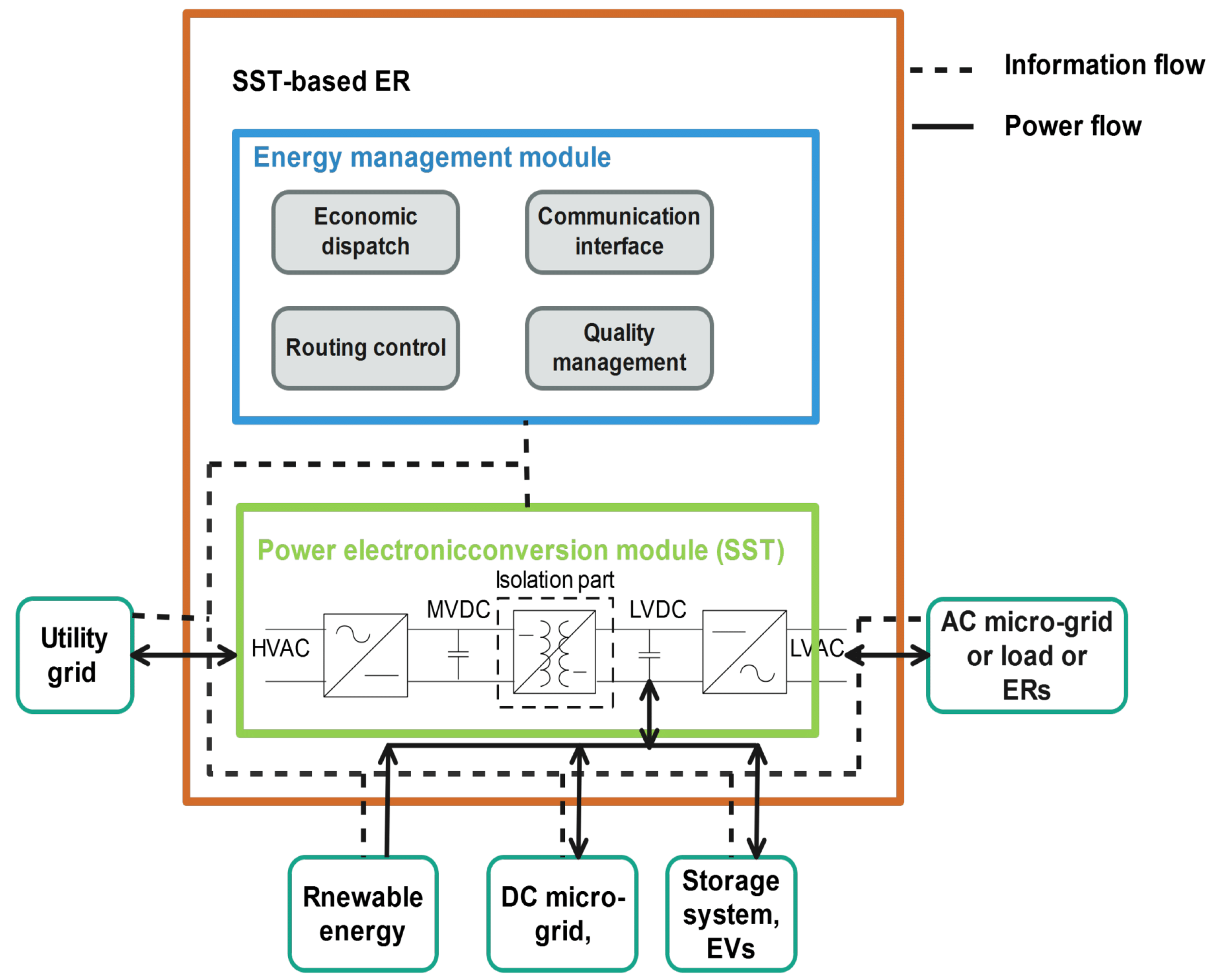
2.2. Energy Router Architecture and Functions

ER is regarded as the primary networking unit for the implementation of the EI. It is proposed to achieve a better utilization of renewable energy sources, with an efficient transmission of energy flows. The ER has comprehensive functions such as an energy exchange, communication and energy management [35]. The study of ERs is in its preliminary stage at present, and various researchers have suggested different ER designs, such as the works in [20,35,36,37]. The common functionalities between the different suggested designs are: the integration of renewable energy sources; the control of power and communication flows; and the regulation of power quality and voltage/frequency conversion.
The first design of ER was based on solid-state transformers (SSTs) and proposed by The Future Renewable Electric Energy Delivery and Management (FREEDM) [38]. As shown in Figure 3, the SST-based ER is composed of an energy management module and power electronic conversion module SST [6,37]. First, the energy management modules can realize the communication, power routing and management using power flow, while the power electronic conversion module (SST) can convert multiple energy forms and voltage levels, as well as compensate for reactive power. It has a three-stage topology: the high-voltage AC/DC stage, the middle DC/DC stage and the low-voltage DC/AC inverter stage. The high-voltage AC/DC stage rectifies the power frequency from High Voltage Alternating Current (HVAC) to Medium Voltage Direct Current (MVDC), the bidirectional middle DC/DC stage transforms the the MVDC to a regulated Low Voltage Direct Current (LVDC), while the low-voltage DC/AC inverters generate a LVAC. The SST provides multiple plug-and-play interfaces that allow loads, storage systems, renewable energy, micro-grids (MGs), utility grid and other ERs to be connected. Every interface can connect various energy systems or devices, provided that the total power connected to the interface does not surpass its capacity limits.
Using ER controlled by information can improve the efficiency of energy transmission and energy allocation. For an efficient energy management, these ERs need to be equipped with efficient dynamic energy routing protocols to respond to changes in energy information, system topology and the regular connection/disconnection of the system devices. For this, in our proposed network architecture, we assume that every ER broadcasts its energy information, its connections (ERs, devices and power links) with their energy information to all other ERs in the system. Whenever the system topology or energy information change, the connected ER broadcasts this information to all the others. Thus, each ER accumulates all the necessary energy information and topology of power system and stores them in two different energy information tables, as shown in Table 2 and Table 3. These tables represent the energy information of the proposed EI in Figure 1 where e f f represents the power conversion efficiency of the corresponding ER converter.

3. Energy Routing Approach

Due to the structure and characteristics of EI, some features must be considered in the routing approach:
  • Energy routing is demand-dominated and the source of energy is not specified;
  • The lost energy cannot be regenerated and may cause an overflow that could lead to the destruction of devices/lines, or even the crash of the whole energy system;
  • The power transmission loss is not only related to the length of the path but also to the transmitted and pre-existing power. Because of this fact, the ERs should not store the routing paths but the energy information of the whole system;
  • The dynamic routing algorithm must achieve the supply–demand balance.
Taking into account these features, we considered the energy routing problem as an optimization problem, where the objective function is to minimize the power transmission losses and cost. To solve this issue, we proposed:
  • A centralized peer-to-peer energy trading architecture;
  • A subscriber matching mechanism for both mono and multi-source consumer cases. This mechanism assigns for each consumer the optimal producer in terms of minimization of both cost and power loss;
  • In the case of multi-source consumer (heavy load), we proposed an energy particle swarm optimization algorithm, to determine the amount of power for a set of producers to achieve minimum power transmission loss and cost;
  • An IACO-based energy routing protocol that ensures a non-congestion efficient-energy transmission.

4. Subscriber Matching Mechanism
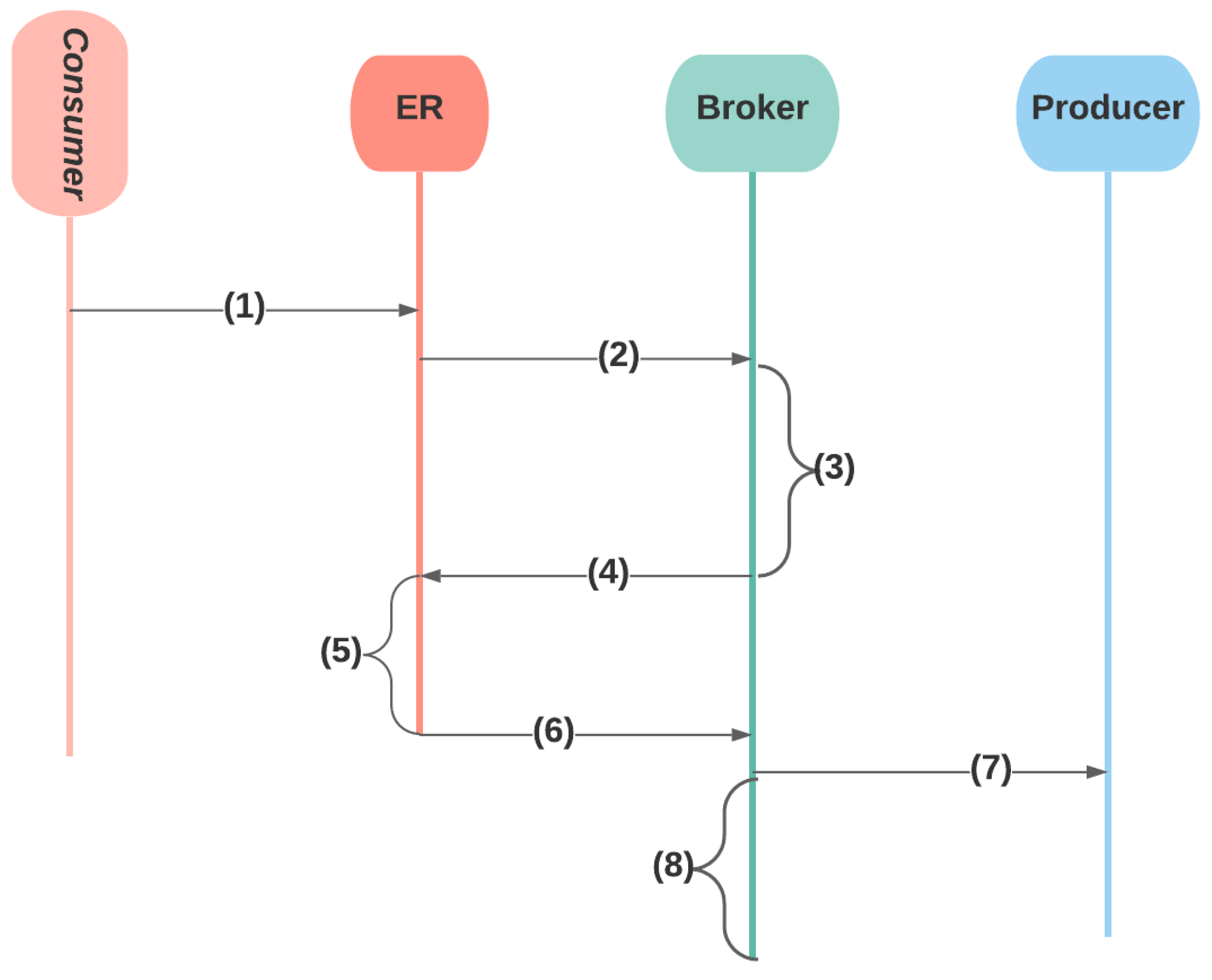
The subscriber matching mechanism constructs the producer (seller)–consumer (buyer) pairs based on the proposed peer-to-peer trading architecture. We assume that, here, the broker stores producers/consumers profiles such as: the electricity price, transmission time and the amount (P) of available/needed power, as shown in Table 4.
As mentioned in the subscriber-matching mechanism sequence diagram (shown in Figure 4):
(1)
Each consumer creates an energy request message with the amount of needed energy, then sends it to their connected ER.
(2)
The ER transfers this energy request to the broker.
(3)
The broker treats the energy demands according to their requesting time and determines for each demand a list of all producers/prosumers that can provide the consumer energy demand in the corresponding time. If there is no single producer/prosumer capable of providing the consumer required energy, then the consumer is a heavy load. In this case, the broker constructs a list of all the producers/prosumers available in the consumer transmission time;.
(4)
The broker sends the constructed list to the consumer energy router.
(5)
After receiving the possible producers’ list, the consumer ER runs the subscriber matching mechanism as illustrated in Algorithm 1,
As illustrated in Algorithm 1, there are two cases:
Algorithm 1: Subscriber Matching Mechanism
Energies 14 02579 i001
Case 1: A mono-source consumer
Here, one or multiple producers can provide the requested energy. Here, ER uses Equation (3) to calculate the fitness value ( F i t n e s s p ) to each producer (p) in the received list.
F i t n e s s p = α × w c p + ( 1 α ) × C o s t p
C o s t p = e l e c t r i c i t y P r i c e × P c × T i m e
where c o s t p and w c p represent, respectively, the cost of energy and the power transmission loss of the best path between the consumer and producer generated by IACO-based energy routing protocol (described in detail in Section 5).
As mentioned in Equation (3), it is evident that the objective function combines two opposing objectives to be minimized: cost and power loss. To make the problem simpler, we connected these two objectives together by an α factor reflecting the degree of importance or weight of each objective, based on the preference of the broker. Thus, for instance, if the broker wants to reduce the C o s t p by giving 80 % of importance to the C o s t p , the importance of the power loss w c p will be just 20 % and α in this case is equal to 0.2 . If the broker wants to give the same importance to the two objectives, α took the value 0.5 .
The broker decides the value of α according to the system generation capacities. Whenever the number of producers or power generation capacity decreases, the degree of power loss importance increases.
(6)
The ER selects the producer with the minimum fitness value (Equation (5)), informs the broker to do the necessary updates (8) and to inform the selected producer (7), creates the virtual circuit to start the transfer of energy using the selected efficient path, updates the pre-existing power in its power tables and informs the other ERs:
M i n i m i z e F i t n e s s p
Case 2: A multi-source consumer (heavy load)
In this case, none of the available prosumers can provide the whole demanded energy, so multiple producers would be chosen by the subscriber matching mechanism to satisfy the consumer demand. The number of selected suppliers for a given consumer (load) should be as limited as possible, to minimize the subscriber matching mechanism complexity, maximize the stability and ensure the security and robustness of the grid [20,21,39]. Using the possible producers list (L), first, the ER creates a vector C n c of a set of producers/prosumers.
C n c = S 1 S 2 S m m × 1 = p 11 p 12 p 1 n p 21 p 22 p 2 n p m 1 p m 2 p m n m × n
Each set S in C n c contains a number of producers (n), where the sum of their available power satisfies the consumer’s demand (6):
Σ k = 1 n P k > = P c , k L
Then, for each set S k in C n c , the ER invokes the energy particle swarm optimization algorithm (EPSOA) to determine the required power amount from each producer in set S k to obtain the minimum fitness value ( F i t n e s s S k ):
F i t n e s s S k = Σ i = 1 n F i t n e s s p i
Algorithms 2 and 3 represent the proposed energy particle swarm optimization algorithm (EPSOA) with its objective function, respectively. The algorithms’ parameters are shown in Table 5.
The EPSOA initially creates k particles. A particle reflects the amount of power to be supplied by each producer in the set S to satisfy the consumer demand (each particle is equivalent to one row in the energy combination matrix). In each particle, if the set contains n producers, the amount of power obtained from producer 1 to producer ( n 1 ) is randomly within the permissible range, while nth producer completes the consumer demand. The algorithm evaluates the fitness value including cost and power loss (Equation (7)) of each particle using the objective function in Algorithm 3, initializes p b e s t and chooses the particle with the minimum fitness value as g b e s t . The algorithm is iterative where in each iteration, the values of X and V are updated using Equations (7) and (8). These equations are taken from [33].
V i t + 1 = w V i t + C 1 r 1 [ p b e s t i t X i t ] + C 2 r 2 [ g b e s t t X i t ]
X i t + 1 = X i t + V i t + 1
The new values of X t + 1 must verify the constraints (10), (11), (13) and (14) while the values of p b e s t and g b e s t are updated as in Algorithm 2.
Algorithm 2: Energy Particle Swarm Optimization
Energies 14 02579 i002
Energies 14 02579 i003
Algorithm 3:EPSOA Objective Function (OF)
Energies 14 02579 i004
  • The total amount of power in the particle must be equal to the consumer demand:
    Σ i = 1 n X i = P c
  • The amount of power from producer j in particle i must be within the producer’s capacity (the available power):
    0 < X i j P p j
Finally, after the determination of the required power amount from each producer in each set with the minimum energy transmission cost, the ER selects the best set using Equation (12):
F i t n e s s m i n = m i n k = 1 m ( F i t n e s s S k )
The ER obtains the best set with all the necessary information (required power, best path to each producer in the best set) and as in case 1, it creates the circuit, does the necessary updates and informs the broker, and then starts the energy transmission from selected producers.
The consumer–prosumer pairs, produced by the subscriber matching, should satisfy the following constraints:
  • If the prosumer/producer is matched with multiple consumers, the total amount of selling electricity ( p c p ) should not exceed the existing power of the prosumer ( P p ):
    0 Σ c = 1 k p c p P p
  • If the consumer is matched with multiple prosumers, the total amount of buying electricity ( p c p ) should not exceed the demand energy of the consumer ( P c ):
    0 Σ p = 1 k p c p P c

5. Improved ACO-Based Energy Routing Protocol (IACO-ERP)

Each ER connected to a consumer executes an IACO-based energy routing algorithm to determine the energy-efficient path between each producer–consumer pair.
In this work, we selected the energy transmission path depending on its power transmission loss. The power transmission loss of a path is related to two main factors: the power lines losses ( w i j ) and ER losses ( w i ) that construct the path. w i j and w i represent the weights of ERs and power lines in the EI model shown in Figure 2.
The power loss in ER is dependent on the conversion efficiency of the electronic converters and the power cable transmission losses inside it. Since the latter is neglected and the conversion efficiency is assumed to be constant, the power loss of ER is a linear function of transmitted power (15). Where we have e f f i , P c p represents the conversion efficiency of router v i and the transmitted power from producer to consumer, respectively:
w i = 1 e f f i × P c p
On the other hand, the total power loss in a power line between energy routers v i and v j is calculated based on the resistance ( R i j ) and reactance ( X i j ) of the line. Since a three-phase grid is used, it was noted that the total power loss of the line is divided into active and reactive power losses:
w i j = P a c t i v e p o w e r l o s s 2 + Q r e a c t i v e p o w e r l o s s 2
with P a c t i v e p o w e r l o s s = 3 × R i j × I 2 and Q r e a c t i v e p o w e r l o s s = 3 × X i j × I 2 . It is known that the reactive power loss is negligible compared to the active power loss and the total power loss in the line becomes:
w i j = 3 × R i j × I 2
Equation (18) describes the relation between the line power loss and the transmitted power:
w i j = R i j V i j 2 × P c p 2
where R i j and V i j are the resistance and voltage of the power line that connect energy routers v i and v j , respectively. However, P c p is the transmitted power of consumer–producer pair. In fact, Equation (18) is not relevant in the case where there is an already existing power ( P i j ) in the line. In this case, the power line loss is calculated using Equation (19):
w i j = R i j V i j 2 × P c p + P i j 2 P i j 2
Accordingly, the total power loss of a transmission path that connects a consumer–prosumer pair is the sum of power losses of all routers and power lines that construct the path.
w c p p a t h = Σ v i p a t h w i + Σ e i j p a t h w i j
To select the minimum loss path between consumer–prosumer pairs, we proposed an improvement of the protocol in [31]. We introduced an improved ACO-based energy routing protocol IACO-ERP, which allows the selection of a non-congestion efficient path, where the objective function is the minimization of the power transmission loss (Equation (21)):
w c p = m i n Σ k p a t h s w c p k
The flowchart in Figure 5 describes the fundamental concept and implementation of the IACO-based energy routing protocol used to find the non-congestion minimum loss path. The relevant parameters are shown in Table 6.
The energy minimum loss path should satisfy the following constraints:
  • The power loss of a path should be less than the transmitted energy:
    w c p p a t h < P c p
  • The transmitted power should not exceed the maximum capacity of the path, which is the minimum between the lowest interface capacity of energy routers and the lowest capacity of the power lines that constructed the path:
    P c p m i n P c p L i n e s _ c , P c p E R s _ c
  • The total power transmitted through a power line should not exceed its available capacity:
    Σ P v i , v j P v i , v j c
  • The total power flows into the same ER interface should not exceed its interface capacity:
    Σ P v i , v j P v i c
The energy routing selection method, in Figure 5, consists of ten steps which are carried out for each consumer–producer pair:
  • First, ERs constructs the network model using the system information (Table 2 and Table 3).
  • Thereafter, receiving the pair information (the amount of transmitted power P c p , identity of the producer/prosumer) and using the constraints (23)–(25), the ER eliminates all edges and nodes(ERs) that cannot transfer the P c p and deducts a sub-graph G2.
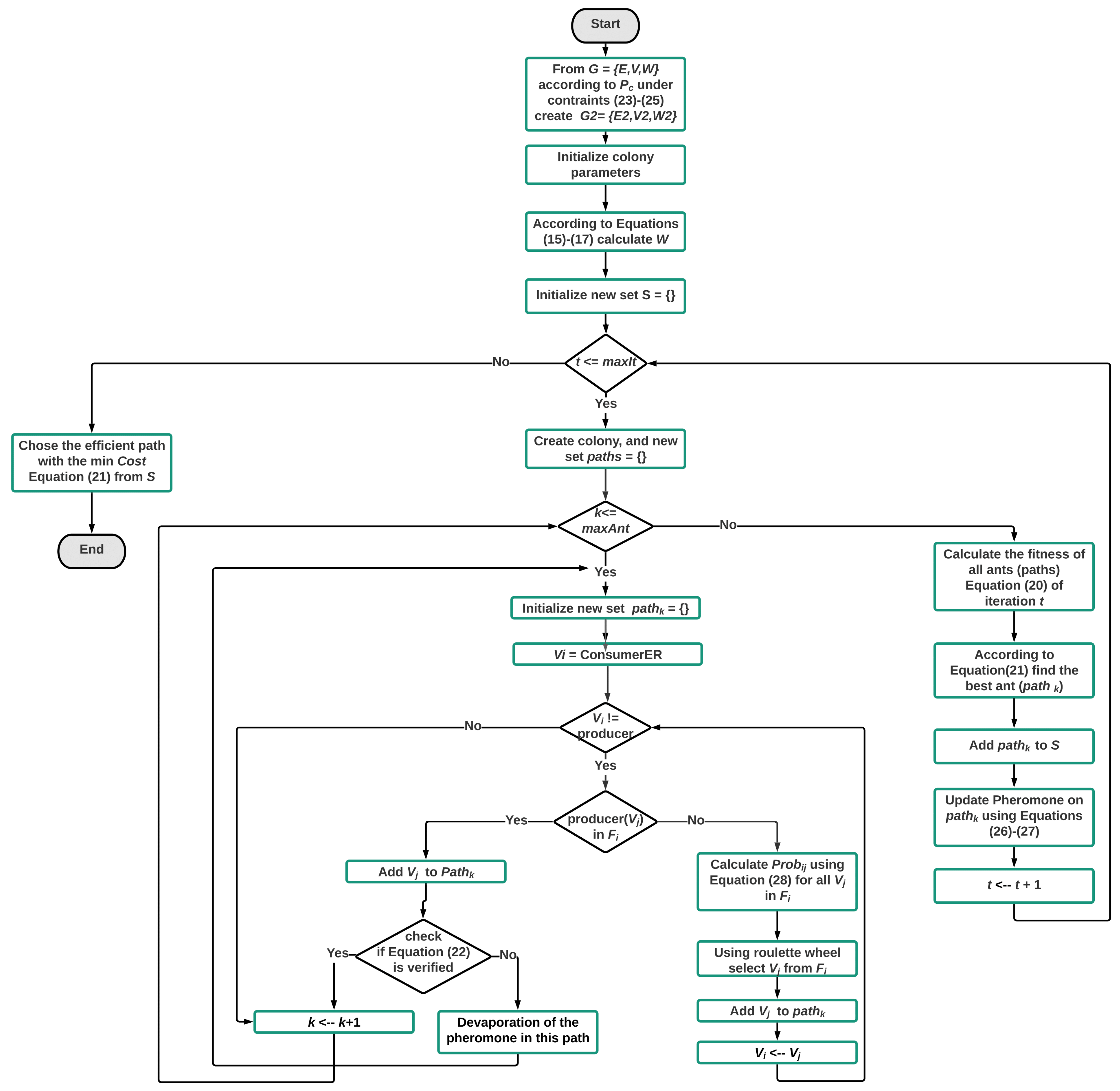
  • The path selection method is based on ACO. Consumers and producers/prosumers represent the ant nest and food source, respectively. Ants are used to determine the best path between them. They use a chemical known as pheromone to communicate and trace the path to the food source. The path with the highest intensity of pheromone is the one widely used by ants. It is usually the shortest path. In nature, some ants depose more pheromones in the case where the food source is big or of higher quality and the path is very good [40]. Therefore, the pheromone level of a path is proportional to its power transmission loss.
    The amount of deposed pheromone on an edge (power line) e i j by ant k is represented by Equation (26):
    Δ t i j k = 1 w p a t h
    where w p a t h is the power transmission loss of the path where the line e i j belongs to this path. When the line e i j connecting routers v i and v j is chosen by an ant k, the amount of pheromone on this line is updated using Equation (27):
    τ i j k = Σ k = 1 n Δ t i j k
    where n represents the number of ants selected on the line e i j .
    In this step, the ER initializes the colony parameters: number of iterations, ants, and pheromone level.
  • Each ant travels from the graph from one node (ER) to another until it arrives to the producer. The selection of the next hop (node) is determined by calculating a probability for each neighbor with the use of the roulette wheel principle. The probability depends on the amount of pheromone and the power loss to the next hop:
    P r o b i j = τ i j α η i j β Σ j F i τ i j α η i j β
    η i j = 1 w i + w i j
    where F i is the neighboring list of node v i , in the graph G 2 , while η i j represents the quality of the power line (edge) e i j , α and β are two parameters that control, respectively, the importance of the pheromone intensity and the quality of the power line.
  • The algorithm runs in iterations, and at each iteration an energy efficient path is selected (set S in Figure 5), and the amount of the pheromone is updated according to Equations (26) and (27).
  • The energy efficient path is the path with the minimum power transmission loss in set S (Equation (21)).
A virtual circuit, constructed using the selected energy efficient path, is allocated to transfer the power between the producer–consumer pair. The exchange information between routers during the creation of energy transmission circuits and the verification of capacity constraints before the construction of the paths prevent the congestion and overhead problems.

6. Algorithms Complexity

Algorithm complexity is one of the metrics used to measure the performance of any given algorithm. In our proposed approach, we have used ACO and PSO algorithms to obtain the best optimal solution. ACO is exploited to find the efficient paths between consumers and their producers. PSO is used to determine the best producers for a heavy load consumer. Despite the fact that the ACO algorithm presents limitations in large-scale combinatorial problems because they require huge processing time, in our case, it outperformed the greedy search algorithm used in [20] to solve the same problem. In what follows, we computed the used algorithms complexity.
We can compute the subscriber matching’s complexity in two cases: heavy loaded network (ComplexHeavy) and light loaded network (ComplexNotHeavy). Since the IACO algorithm is invoked in both cases, let us compute its complexity first. Assume n is the number of ER nodes, m is the number of ants, and the maximum number of iteration is maxit. Then, the time complexity analysis of IACO algorithm is: O ( n × ( n 1 ) × m × m a x i t / 2 )
(1)
The time complexity of the light-loaded network is (see Table 7):
C o m p l e x N o t H e a v y = 1 + n p × ( 1 + c o m I A C O + 1 ) + 1 = 2 + 2 × n p + n p × c o m I A C O = 2 + 2 × n p + n p × O ( n × ( n 1 ) × m × m a x i t / 2 ) = O ( n 2 × m × m a x i t / 2 ) b e c a u s e 2 + 2 × n p i s l e s s t h a n c o m I A C O .
where np is the number of possible producers.
(2)
The time complexity of the heavy loaded network is (the worst scenario (see Table 8)):
C o m p l e x H e a v y = c o m p ( C ( c , n ) ) + m × c o m p ( E P S O A ) + c o m p ( E P S O A o b j e c t i v e f u n c t i o n ) + 1 = O ( n m i n ( c , c n ) ) + m × O ( m a x i t × k × n p ) + O ( n 2 × m × m a x i t / 2 ) + 1
where:
  • c o m p ( C ( c , n ) ) = O ( n m i n ( c , c k ) ) is the combination complexity.
  • comp(EPSOA) is the EPSOA algorithm complexity. TheEPSOA algorithm contains several elementary instructions, two nested loops and three nested loops. Then, its complexity is O(maxit × k × np) (see Table 9):
    c o m p ( E P S O A ) = 1 + O ( k × n ) + O ( k ) + 4 + 5 × O ( m a x i t ) + 3 × O ( k × m a x i t ) + 2 × O ( m a x i t × k × n p ) = O ( m a x i t × k × n p )
    where k is the number of particles.
  • comp(EPSOA objective function) is the same as the complexity of the light loaded network case, previously computed as:
    c o m p ( E P S O A o b j e c t i v e f u n c t i o n ) = O ( n 2 × m × m a x i t / 2 )

7. Simulation and Results

In this section, various study cases, implemented in MATLAB, were conducted to validate the effectiveness of the proposed energy routing approach. Additionally, the comparison to an existing routing algorithm is carried out to evaluate the performance of the proposed approach. The ER-based EI represented in Figure 1 is treated as a simulation case where the energy system parameters are:

7.1. Basic Data

Table 2 and Table 3 illustrate the parameters of power lines and ERs used in the proposed EI (Figure 1). On the other hand, Table 10 lists the energy profile of producers/consumers in the proposed network, including the cost, power and required transmission time.

7.2. Results of the Proposed Energy Routing Approach

Applying the proposed energy routing approach, a source selection (Section 4) with a non-congestion minimum loss path (Section 5) is constructed for each consumer.
Case 1 analysis: mono-source consumer with non overlapping transmission time
In this case, according to Table 10, there are two consumers (D7 and D3) with two producers (D2 and D4). The transmission time of the consumers is different, which means it does not have any overlap. Thus, in this case, the pre-existing power through lines is zero and the energy transmission path taken by the first consumer will not affect the second one. Starting with consumer D7, using the proposed energy routing mechanism:
  • D7 sends energy request to E R 17 .
  • E R 17 transfers this request to the broker.
  • The broker creates a list with the available producers that can provide 12 kw in the corresponding time (10.00–12.00) L = { D 2 , D 4 } , and sends it to E R 17 .
  • E R 17 
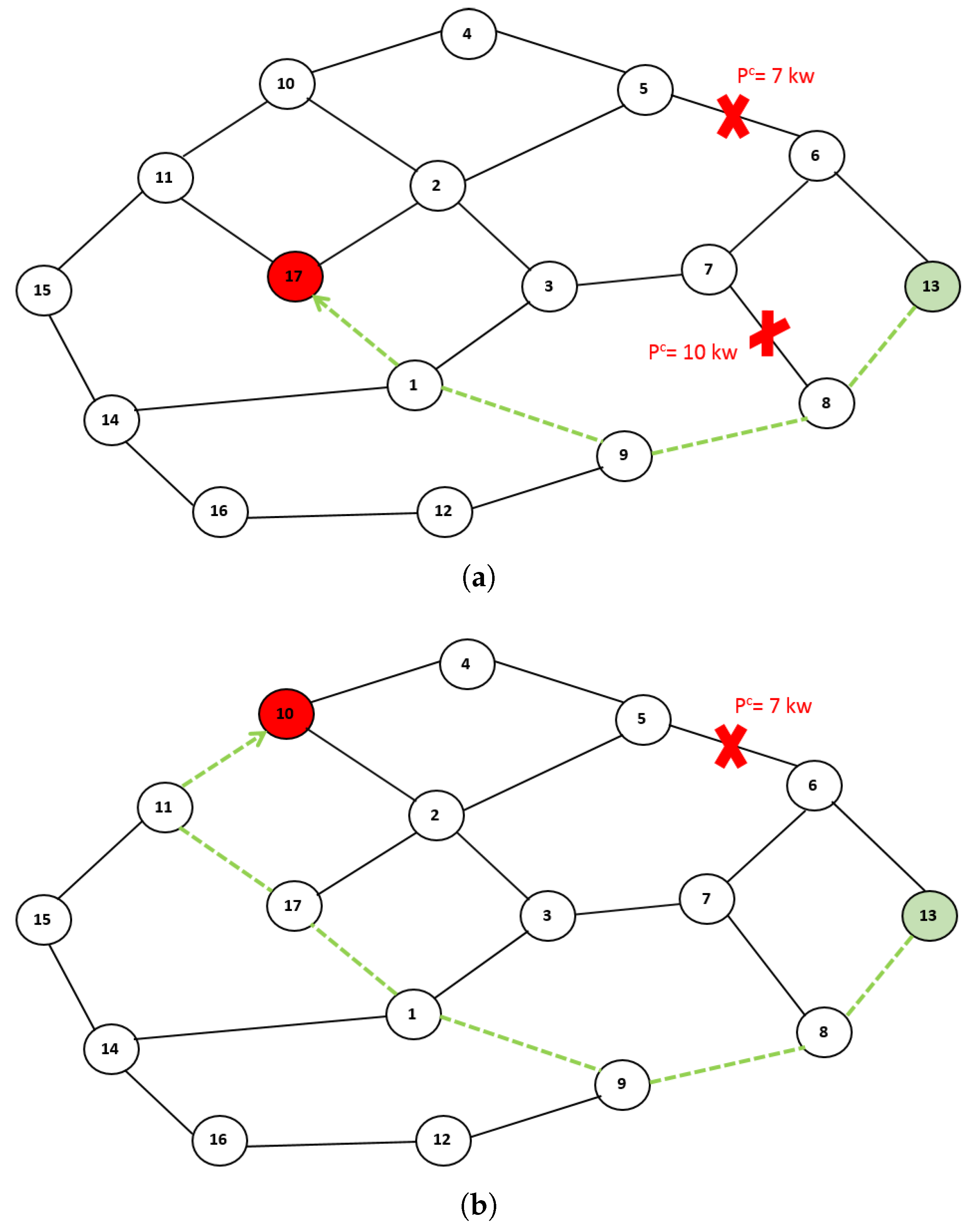
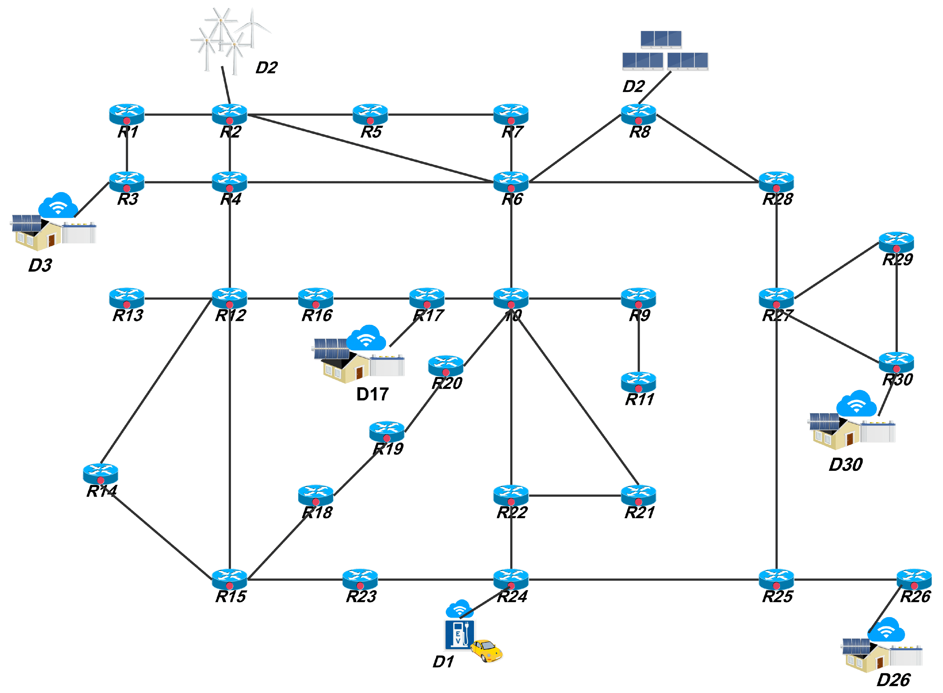
starts the execution of the subscriber matching mechanism (Section 4). As we can see, D7 is a mono-source consumer. Thus, for each producer in L (D2 and D4), the E R 17 calculates the cost and the energy-efficient path to determine the fitness value. The energy-efficient path is given by the execution of IACO-based energy routing protocol (IACO-ERP) described in Section 5. The protocol’s first phase allows the E R 17 to construct a new graph from the EI graph (Figure 2) by deleting all the lines and routers that cannot transfer 12 kw as shown in Figure 6. This step with the dynamic routing creates a non-congestion minimum loss path.
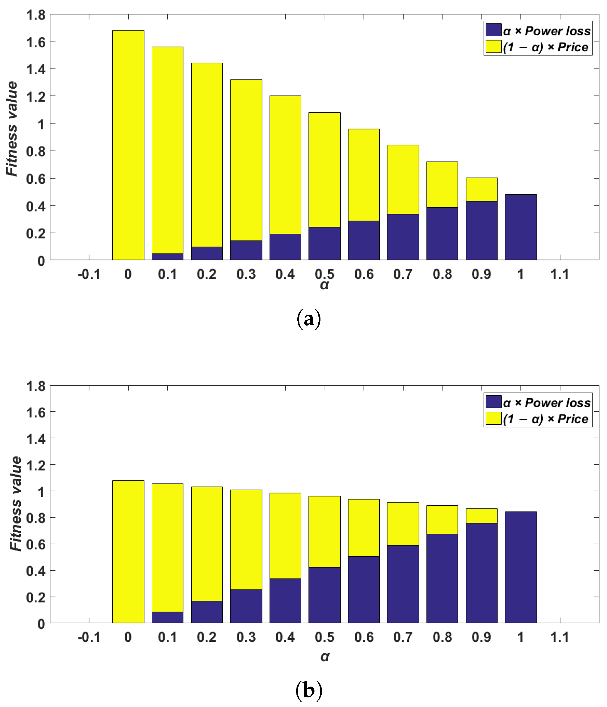
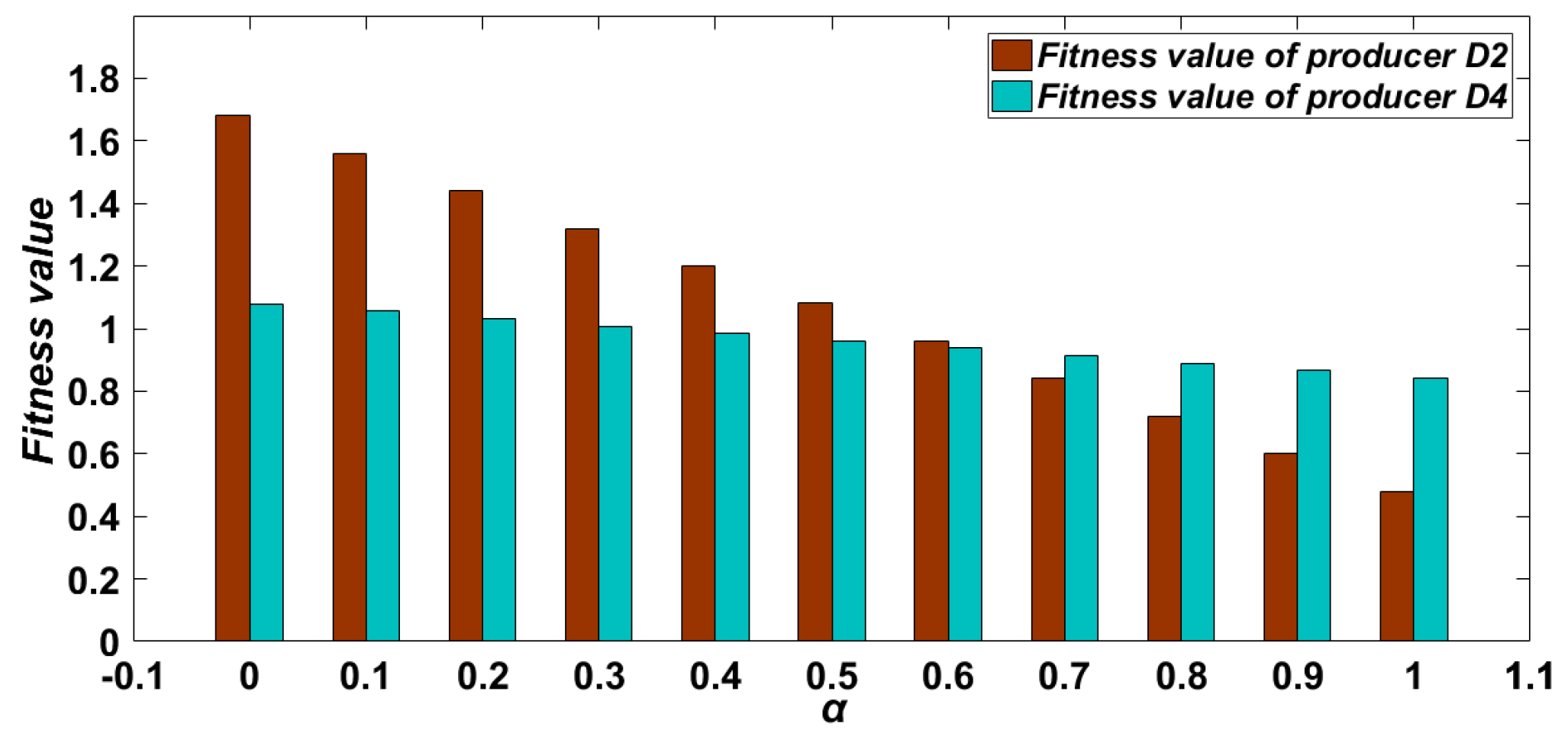
  • As described in Equation (3), in our approach, the objective was the minimization of the power loss and cost of energy. For that, the value of α used in the calculation of the fitness value was 0.5 . With this value, E R 17 selects the producer D 4 with the fitness value for consumer D 7 .
    The same process is repeated for consumer D 3 with E R 10 .
The calculation results including costs, efficient paths, power losses and selected sources, transmission power and the max capacity of paths are shown in Table 11 and Figure 6. The selected producers with the efficient paths for consumer D7 and D3 satisfied the energy routing constraints.
As illustrated in Figure 7 and Figure 8, the variation of α from 0 to 1 shows that the degree of the importance of the cost and power loss progresses in the opposite direction, which affects the producer selection. There are two special cases when α = 0 or α = 1 :
  • α = 0 : The fitness value depends only on the cost of energy, in this case, the producer with the minimum fitness value is producer D4.
  • α = 1 : The fitness value depends only on the power transmission loss of the best path, in this case, the producer with the minimum fitness value is producer D2.
Case 2 analysis: mono-source consumer with overlapping transmission time
Consumers D3 and D7 have an overlapping transmission time (case 2 in Table 10). Thus, the pre-existing power over certain power lines may be different from zero. This will lead to major changes of the power loss in those lines, which directly affect the efficient path selection; therefore, affecting the fitness value responsible for the producer selection.
By comparison to case 1, as shown in Table 12 and Figure 9, the selected producer for consumer D7 is D4 with the same energy efficient path, power loss and fitness value since, at the beginning, the pre-existing power in this path is equal to zero. However, across the overlapping time, the energy-efficient transmission paths from D3 to D2 and D4 have changed from the original paths 9 → 1 → 17 → 11 → 10, and 13 → 8 → 9 → 1 → 17 → 11 → 10, to 9 → 1 → 3 → 2 → 10 and 13 → 6 → 7 → 3 → 2 → 10, respectively. Because of the change in the pre-existing power in 13 → 8 → 9 → 1 → 17, from 0 to 12 kw, which results in increasing in the power losses of those power lines, has led to an augmentation in the power loss of the original efficient paths, which have become 5.61296 × 10 1 kw and 8.0264 × 10 1 kw, respectively, which influenced the fitness value.
The results of cases 1 and 2 demonstrated that the power loss in the power system was not only affected by the energy transmitted, but also by the pre-existing power.
Case 3 analysis: congestion management
Energy transmission congestion can occur in energy systems when the transmitted power exceeds the capacity of the transmission paths, known as the overflow problem. This could have serious consequences in the energy system. As illustrated in Table 10, in this simulation case, it is assumed that there is an overlapping transmission time such as in case 2, and the capacity of power lines L 3 7 and L 8 13 are restricted to 12 kw and 6 kw, respectively.
As mentioned before in Section 5, the IACO-based energy routing protocol eliminates all the ERs and lines that cannot support the transmitted power from the network before finding the efficient path to avoid the overflow problem, and to ensure the selection of a non-congestion minimum loss path. Table 13 and Figure 10 summarize the results for this case. By comparison to case 2, we can state that:
  • Consumers D3 and D7 have the same transmission power.
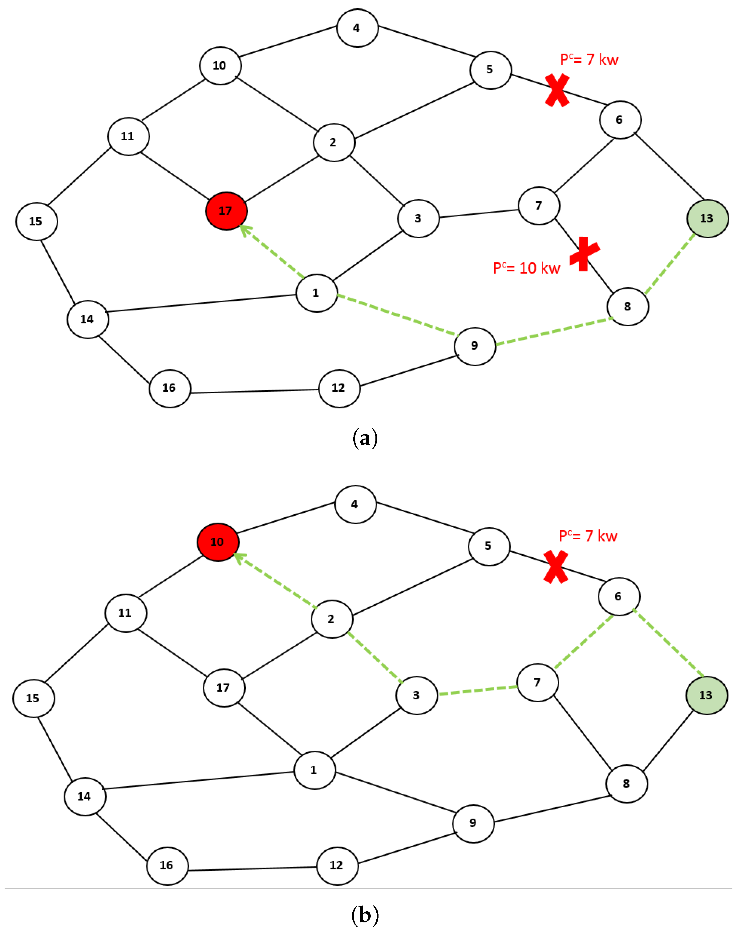
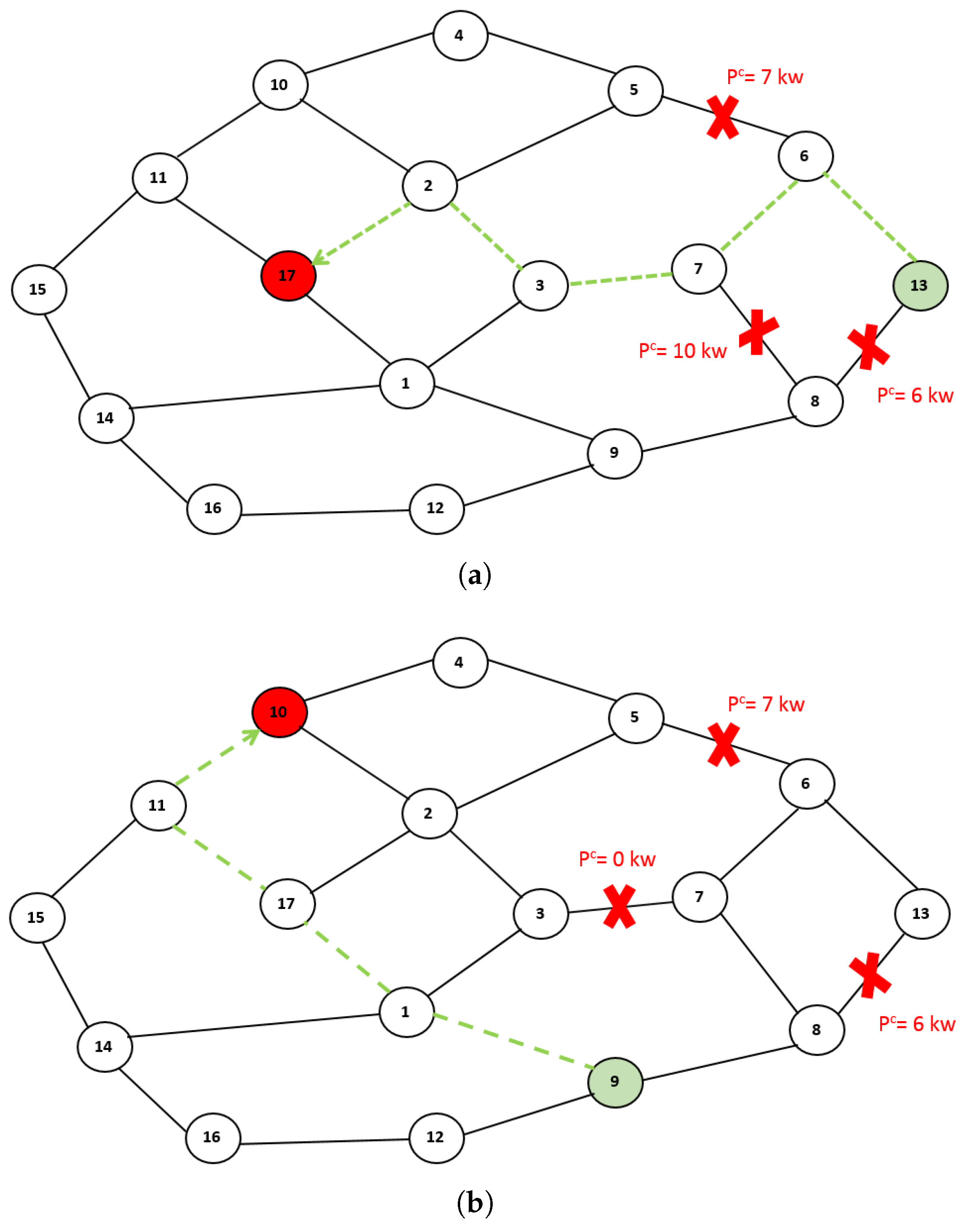
  • For consumer D7, the efficient path from D7 to D2 is the same as in case 2. While, the path toward D4 (13 → 8 → 9 → 1 → 17), cannot be used in this transaction since the transmission power (12 kw) exceeds the capacity of line L 8 13 (6 kw). Therefore, it has been replaced by another path with higher power transmission loss, which causes an increase in the energy transmission cost.
  • For consumer D3, as shown in Figure 10a, D7 selected the producer D4 with the efficient path 13 → 6 → 7 → 3 → 1 → 17. In this situation, the power line L 3 7 reaches its maximum capacity, so it is not available to be shared. Therefore, E R 10 turns from the path in case 2 (13 → 6 → 7 → 3 → 2 → 10) to a new path (Table 13) with a higher loss resulting in a higher fitness value. Since consumer D7 changed the selected path compared with case 2, this creates the opportunity to find a new path with minimal loss between D3 and D2 (see Table 13 and Figure 10b). As a result, D3 turns to consumer D2 with a minimum fitness value.
Case 4 analysis: multi-source consumer
In order to validate the effectiveness of the proposed energy routing approach in multi-source consumer cases, we considered the electric vehicle (EV) as a heavy load with a charging request of 22 kw (according to the European EV charging standard IEC 61851 [41]). As shown in Table 14, we assume that there are three producers and none of them can provide the requested power. In this case, more than one producer should be selected to satisfy the EV demand power (D1). Consumer D1 (EV) requests the required power using E R 4 . In contrast to the previous cases, the broker list in this case contains all the producers that are available in the EV transmission time ( L = { D 2 , D 5 , D 6 } ). According to the power information of the producers in L, at least two sources are needed to provide the requested amount of power by the consumer. Therefore, after receiving the list ( L = { D 2 , D 5 , D 6 } ), E R 4 using Equation (6) creates a combination set as
C 2 D 1 = S 1 S 2 2 × 1 = D 2 D 6 D 5 D 6 2 × 2
There are two possible sources combination sets ( S 1 , S 2 ). According to the Equation (3), the fitness value is calculated using a function that optimizes the cost and power loss. Therefore, for each set S i the E R 4 invokes the EPSOA to define the optimum amount of power that should be collected from each producer in the S i where this amount of power optimizes the fitness value ( F i t n e s s S i ) as well as satisfies the consumer demand.
Table 15 shows the simulation results of multi-source consumer case, however, Table 16 represents the IACO-based energy routing protocol and EPSOA simulation parameters.
As shown in Table 15, the fitness value of S 1 is larger than the fitness value of S 2 . Thus, E R 4 chooses the set S 2 with the power and paths allocation shown in Figure 11:
p D 5 = 11.9928 kw p a t h ( D 5 : D 1 ) : 15 11 10 4 p D 6 = 10.0072 kw p a t h ( D 6 : D 1 ) : 16 14 1 3 2 5 4
Table 17, Table 18 and Table 19 show the variation of α and its affect on the results of EPSOA. Figure 12 shows the convergence of the EPSOA in the two sets.
Case 5 analysis: 30 nodes system structure
The 30-node (ERs) system was used for further study to validate the efficacy of the proposed energy routing approach on a more complex system, as shown in Figure 13. Table 20 and Table 21 show the power lines and ERs parameters used for system in Figure 13. In this system, there are two mono-source consumers, one multi-source consumer and four surplus-energy prosumers. Table 22 displays their energy profile including their cost, power and required transmission time.
In case 1 in Table 22, the transmission time of the different consumers does not have an overlapping time. Thus, the different energy transactions will not affect each other during the selection of the minimum energy loss transmission path.
Table 23 illustrates the optimization results of the proposed approach with α = 0.5 . The constructed pairs with the transmission paths that all energy routing constraints such as the power loss and capacity constraints.
However, in case 2 in Table 22, there is an overlapping time between the transmission time of consumers. Consumer D 26 was supplied by producer D 30 through the same energy-efficient path as in case 1 ( 30 27 25 26 ). In this case, the left capacity in the power line was L 27 25 = 9 kw and it cannot be used to transfer the required energy (see case 1 in Table 23) from prosumer D 8 to consumer D 24 . Thus, another non-congestion energy-efficient path with a different energy amount was constructed using EPSOA and the IACO in set S 1 for consumer D 24 . Since the new solution for set S 1 has higher fitness function, the selected set for consumer D 24 is set S 2 . For consumer D 7 , the only prosumer that can provide the demand in the corresponding time is D 2 .

7.3. Results Discussion

In order to validate the performance of our proposed scheme, as well as to show its efficiency in solving problems related to energy routing, namely subscriber matching, efficient routing path and transmission scheduling, we compared the obtained results of different experiments to previous works in the literature.
As illustrated in Table 24, starting with the mono-source consumer case, works in [20,21] have proposed an energy routing protocols based on graph traversal and Dijkstra algorithms, respectively, to determine a non congestion minimum loss path between producer–consumer pairs. First, the two proposed protocols did not examine how pairs were formed. The graph traversal method in [20] finds that all possible paths between the producer and consumer pairs then determines the path with the minimum power loss. This method generates an optimal solution but with a height execution time especially in the case of large-scale networks. IACO-ERP offers the best solution compared to [20] with the same execution time for small-scale networks and a better execution time for large-scale networks as shown in Table 25. In addition, we proposed a subscriber matching mechanism that decides which producer should be chosen for the consumer while reducing the costs and losses of energy.
For the multi-source consumer, the work in [20] proposed a source selection algorithm that determines the amount of power to obtain from each producer to satisfy the heavy load demand. The proposed algorithm used the greedy search topology where it tests all possible (interval values) cases to define the appropriate amount of power that needs to be received from each producer in the aim of minimizing the power loss. This method provides a solution with a high execution time which speedily augments with the growing of the system. The execution time of cases 4 and 5 is 217 s and 513 s, respectively, whereas using the EPSOA algorithm helped in achieving the best solution in a significantly reduced time while minimizing the cost and power loss at the same time. Our proposed scheme produced the same result for cases 4 and 5 in 51 s and 109 s seconds of execution time, respectively. In comparison with fully distributed peer–peer energy trading, the use of the broker minimized the number of exchange messages in the system.

8. Conclusions and Future Work

With the expanded use of renewable energy sources in EI, the centralized energy supply mode has shifted to a multi-source and multi path mode leading to the peer-to-peer energy trading market. The energy routing process is one of the major problems faced in EI. To solve this problem, we proposed a solution to the three issues: subscriber matching, energy-efficient path and transmission scheduling. For this purpose, we developed a centralized peer-to-peer energy trading scheme that uses a central broker and novel energy routing approach. The energy routing approach is based on meta-heuristic method to achieve a P2P energy trading with an efficient routing in the EI with respect to the energy routing constraints and congestion. The main objective of the proposed approach is to reduce the energy cost and losses while satisfying the consumers request. The use of a meta-heuristic method reduces the execution time. In fact, the energy routing approach is composed of three algorithms, the first one is the subscriber matching mechanism that determines the producer–consumer pairs with the minimization of the cost and losses of energy for both mono and multi-source consumers. The non-congestion energy minimum loss path between producer–consumer pairs is generated by the IACO-ERP. In the case of multi-source consumers such as EVs where none of the existing producers can provide the required energy, two or more producers should be selected to supply the requested amount of power. For that, the EPSOA determines the appropriate producers to achieve the lowest energy cost and losses. The effectiveness of the proposed approach, in terms of cost, power losses and congestion management, is verified by different cases analysis. The overlapping time provides a better utilization of network power lines with more power losses compared to the non-overlapping time. In addition, the use of the broker decreases the number of messages exchanged in the network. By comparison to the work in [20], our proposed approach has improved the execution time for both mono- and multi-sources cases in small and large systems by 7 min. The proposed approach can be used to match prosumers in the local energy market, provide alternative transmission paths when the efficient path is disrupted, and manage congestion on distribution links.
In the future, we plan to explore the possibility of applying additional bio-inspired methods, and we aim to explore to apply our solution to real life applications.

Author Contributions

The specific contributions made by each author are shown as follows: conceptualization, D.M.; formal analysis, S.H. (Sara Hebal); methodology, S.H. (Sara Hebal); software, S.H. (Sara Hebal); supervision, S.H. (Saad Harous); visualization, M.D.; writing—original draft, S.H. (Sara Hebal); writing—review and editing, D.M. All authors have read and agreed to the published version of the manuscript.

Funding

This research received no external funding.

Institutional Review Board Statement

Not applicable.

Informed Consent Statement

Not applicable.

Data Availability Statement

No new data were created or analyzed in this study. Data sharing is not applicable to this article.

Conflicts of Interest

The authors declare no conflict of interest.

Abbreviations

The following abbreviations were used in this manuscript:
ACOAnt Colony Optimization
DREsDistributed Renewable Energy sources
EIEnergy Internet
EPSOAEnergy Particle Swarm Optimization Algorithm.
EREnergy Router
HVACHigh Voltage Alternating Current
IACO-ERPImproved Ant Colony Optimization Energy Routing Protocol.
LVDCLow Voltage Direct Current
MVDCMedium Voltage Direct Current
PSOParticle Swarm Optimization
SGSmart Grid
SSTSolid State Transformer

References

  1. Tushar, W.; Chai, B.; Yuen, C.; Smith, D.B.; Wood, K.L.; Yang, Z.; Poor, H.V. Three-party energy management with distributed energy resources in smart grid. IEEE Trans. Ind. Electron. 2014, 62, 2487–2498. [Google Scholar] [CrossRef] [Green Version]
  2. Wang, K.; Yu, J.; Yu, Y.; Qian, Y.; Zeng, D.; Guo, S.; Xiang, Y.; Wu, J. A survey on energy internet: Architecture, approach, and emerging technologies. IEEE Syst. J. 2017, 12, 2403–2416. [Google Scholar] [CrossRef]
  3. Surani, R.R. From Smart Grids to an Energy Internet: A Review Paper on Key Features of an Energy Internet. Int. J. Eng. Res. Technol. 2019, 8, 228–231. [Google Scholar]
  4. Rifkin, J. The Third Industrial Revolution: How Lateral Power Is Transforming Energy, the Economy, and the World; Macmillan: Stuttgart, Germany, 2011. [Google Scholar]
  5. Chen, Z.; Liu, Q.; Li, Y.; Liu, S. Discussion on energy internet and its key technology. J. Power Energy Eng. 2017, 5, 1–9. [Google Scholar] [CrossRef] [Green Version]
  6. Tsoukalas, L.; Gao, R. From smart grids to an energy internet: Assumptions, architectures and requirements. In Proceedings of the 2008 Third International Conference on Electric Utility Deregulation and Restructuring and Power Technologies, Nanjing, China, 6–9 April 2008; pp. 94–98. [Google Scholar]
  7. Zhou, Y.; Wu, J.; Long, C.; Ming, W. State-of-the-art analysis and perspectives for peer-to-peer energy trading. Engineering 2020, 6, 739–753. [Google Scholar] [CrossRef]
  8. Cui, C.X. The UK Electricity Markets: Its Evolution, Wholesale Prices and Challenge of Wind Energy; University of Stirling: Stirling, UK, 2010. [Google Scholar]
  9. Ye, L.C.; Rodrigues, J.F.; Lin, H.X. Analysis of feed-in tariff policies for solar photovoltaic in China 2011–2016. Appl. Energy 2017, 203, 496–505. [Google Scholar] [CrossRef]
  10. Wu, J.; Zhou, W.; Zhong, W.; Liu, J. Multi-energy demand response management in energy Internet: A stackelberg game approach. Chin. J. Electron. 2019, 28, 640–644. [Google Scholar] [CrossRef]
  11. Irtija, N.; Sangoleye, F.; Tsiropoulou, E.E. Contract-Theoretic Demand Response Management in Smart Grid Systems. IEEE Access 2020, 8, 184976–184987. [Google Scholar] [CrossRef]
  12. Tushar, W.; Saha, T.K.; Yuen, C.; Smith, D.; Poor, H.V. Peer-to-peer trading in electricity networks: An overview. IEEE Trans. Smart Grid 2020, 11, 3185–3200. [Google Scholar] [CrossRef] [Green Version]
  13. Abdella, J.; Shuaib, K. Peer to peer distributed energy trading in smart grids: A survey. Energies 2018, 11, 1560. [Google Scholar] [CrossRef] [Green Version]
  14. Zhang, C.; Wu, J.; Zhou, Y.; Cheng, M.; Long, C. Peer-to-Peer energy trading in a Microgrid. Appl. Energy 2018, 220, 1–12. [Google Scholar] [CrossRef]
  15. Wang, N.; Xu, W.; Xu, Z.; Shao, W. Peer-to-peer energy trading among microgrids with multidimensional willingness. Energies 2018, 11, 3312. [Google Scholar] [CrossRef] [Green Version]
  16. Shrestha, A.; Bishwokarma, R.; Chapagain, A.; Banjara, S.; Aryal, S.; Mali, B.; Thapa, R.; Bista, D.; Hayes, B.P.; Papadakis, A.; et al. Peer-to-peer energy trading in micro/mini-grids for local energy communities: A review and case study of Nepal. IEEE Access 2019, 7, 131911–131928. [Google Scholar] [CrossRef]
  17. Tushar, W.; Yuen, C.; Saha, T.K.; Morstyn, T.; Chapman, A.C.; Alam, M.J.E.; Hanif, S.; Poor, H.V. Peer-to-peer energy systems for connected communities: A review of recent advances and emerging challenges. Appl. Energy 2021, 282, 116131. [Google Scholar] [CrossRef]
  18. Huang, A.Q. Solid state transformers, the Energy Router and the Energy Internet. In The Energy Internet; Elsevier: Amsterdam, The Netherlands, 2019; pp. 21–44. [Google Scholar]
  19. Guo, H.; Wang, F.; Zhang, L.; Luo, J. A hierarchical optimization strategy of the energy router-based energy Internet. IEEE Trans. Power Syst. 2019, 34, 4177–4185. [Google Scholar] [CrossRef]
  20. Wang, R.; Wu, J.; Qian, Z.; Lin, Z.; He, X. A graph theory based energy routing algorithm in energy local area network. IEEE Trans. Ind. Inform. 2017, 13, 3275–3285. [Google Scholar] [CrossRef] [Green Version]
  21. Guo, H.; Wang, F.; James, G.; Zhang, L.; Luo, J. Graph theory based topology design and energy routing control of the energy internet. IET Gener. Transm. Distrib. 2018, 12, 4507–4514. [Google Scholar] [CrossRef]
  22. Lin, J.; Yu, W.; Griffith, D.; Yang, X.; Xu, G.; Lu, C. On distributed energy routing protocols in the smart grid. In Software Engineering, Artificial Intelligence, Networking and Parallel/Distributed Computing; Springer: Berlin/Heidelberg, Germany, 2013; pp. 143–159. [Google Scholar]
  23. Sivanantham, G.; Gopalakrishnan, S. A Stackelberg game theoretical approach for demand response in smart grid. Pers. Ubiquitous Comput. 2019, 24, 511–518. [Google Scholar] [CrossRef]
  24. Apostolopoulos, P.A.; Tsiropoulou, E.E.; Papavassiliou, S. Demand response management in smart grid networks: A two-stage game-theoretic learning-based approach. Mob. Netw. Appl. 2018, 1–14. [Google Scholar] [CrossRef] [Green Version]
  25. Hong, J.S.; Kim, M. Game-theory-based approach for energy routing in a smart grid network. J. Comput. Netw. Commun. 2016, 2016, 4761720. [Google Scholar] [CrossRef] [Green Version]
  26. Ma, J.; Song, L.; Li, Y. Optimal power dispatching for local area packetized power network. IEEE Trans. Smart Grid 2017, 9, 4765–4776. [Google Scholar] [CrossRef]
  27. Tushar, W.; Saha, T.K.; Yuen, C.; Morstyn, T.; Poor, H.V.; Bean, R. Grid influenced peer-to-peer energy trading. IEEE Trans. Smart Grid 2019, 11, 1407–1418. [Google Scholar] [CrossRef] [Green Version]
  28. Tushar, W.; Saha, T.K.; Yuen, C.; Azim, M.I.; Morstyn, T.; Poor, H.V.; Niyato, D.; Bean, R. A coalition formation game framework for peer-to-peer energy trading. Appl. Energy 2020, 261, 114436. [Google Scholar] [CrossRef] [Green Version]
  29. Brocco, A. Fully distributed power routing for an ad hoc nanogrid. In Proceedings of the 2013 IEEE International Workshop on Inteligent Energy Systems (IWIES), Vienna, Austria, 14 November 2013; pp. 113–118. [Google Scholar]
  30. Lin, C.C.; Wu, Y.F.; Liu, W.Y. Optimal sharing energy of a complex of houses through energy trading in the Internet of energy. Energy 2021, 220, 119613. [Google Scholar] [CrossRef]
  31. Hebal, S.; Mechta, D.; Harous, S. ACO-based Distributed Energy Routing Protocol In Smart Grid. In Proceedings of the 2019 IEEE 10th Annual Ubiquitous Computing, Electronics & Mobile Communication Conference (UEMCON), New York, NY, USA, 10–12 October 2019; pp. 0568–0571. [Google Scholar]
  32. Hebal, S.; Harous, S.; Mechta, D. Latency and Energy Transmission Cost Optimization using BCO-aware Energy Routing for Smart Grid. In Proceedings of the 2020 International Wireless Communications and Mobile Computing (IWCMC), Limassol, Cyprus, 15–19 June 2020; pp. 1170–1175. [Google Scholar] [CrossRef]
  33. Mechta, D.; Harous, S.; Hebal, S. Energy-efficient path-aware routing Protocol based on PSO for Smart Grids. In Proceedings of the 2020 IEEE International Conference on Electro Information Technology (EIT), Chicago, IL, USA, 31 July–1 August 2020; pp. 093–097. [Google Scholar] [CrossRef]
  34. Dhriyyef, M.; El Mehdi, A.; Elhitmy, M.; Elhafyani, M. Management strategy of power exchange in a building between grid, photovoltaic and batteries. In International Conference on Electronic Engineering and Renewable Energy; Springer: Singapore, 2020; pp. 831–841. [Google Scholar]
  35. Liu, Y.; Li, Y.; Liang, H.; He, J.; Cui, H. Energy routing control strategy for integrated microgrids including photovoltaic, battery-energy storage and electric vehicles. Energies 2019, 12, 302. [Google Scholar] [CrossRef] [Green Version]
  36. Liu, Y.; Wu, Y.; Yang, K.; Bi, C.; Chen, X.; Zhao, Y. Novel Energy Router with Multiple Operation Modes. Energy Procedia 2019, 158, 2586–2591. [Google Scholar] [CrossRef]
  37. Guo, H.; Wang, F.; Luo, J.; Zhang, L. Review of energy routers applied for the energy internet integrating renewable energy. In Proceedings of the 2016 IEEE 8th International Power Electronics and Motion Control Conference (IPEMC-ECCE Asia), Hefei, China, 22–26 May 2016; pp. 1997–2003. [Google Scholar]
  38. Huang, A.Q.; Crow, M.L.; Heydt, G.T.; Zheng, J.P.; Dale, S.J. The future renewable electric energy delivery and management (FREEDM) system: The energy internet. Proc. IEEE 2010, 99, 133–148. [Google Scholar] [CrossRef]
  39. Razi, R.; Pham, C.; Hably, A.; Bacha, S.; Tran, Q.T.; Iman-Eini, H. A Novel Graph-based Routing Algorithm in Residential Multi-Microgrid Systems. IEEE Trans. Ind. Inform. 2020, 17, 1774–1784. [Google Scholar] [CrossRef]
  40. Dorigo, M.; Birattari, M. Ant Colony Optimization. Encyclopedia of Machine Learning; Springer: New York, NY, USA, 2010. [Google Scholar]
  41. Falvo, M.C.; Sbordone, D.; Bayram, I.S.; Devetsikiotis, M. EV charging stations and modes: International standards. In Proceedings of the 2014 International Symposium on Power Electronics, Electrical Drives, Automation and Motion, Ischia, Italy, 18–20 June 2014; pp. 1134–1139. [Google Scholar]
Figure 1. Example structure of the proposed Energy Internet.
Energies 14 02579 g001
Figure 2. Energy Internet model.
Energies 14 02579 g002
Figure 3. SST-based ER architecture.
Energies 14 02579 g003
Figure 4. Energy routing approach sequence diagram.
Energies 14 02579 g004
Figure 5. Improved ACO-based energy routing protocol (IACO-ERP).
Energies 14 02579 g005
Figure 6. Optimization results of case 1 ( α = 0.5 ): (a) energy-efficient path from D4 ( E R 13 ) to D7 ( E R 17 ); (b) energy-efficient path from D4 ( E R 13 ) to D3 ( E R 10 ).
Energies 14 02579 g006
Figure 7. Fitness value for D7 based on the variation of α : (a) for producer D2; (b) for producer D4.
Energies 14 02579 g007
Figure 8. D2 and D4 Fitness values for D7 based on α variation.
Energies 14 02579 g008
Figure 9. Optimization results of case 2 ( α = 0.5 ): (a) energy-efficient path from D4 ( E R 13 ) to D7 ( E R 17 ); (b) energy-efficient path from D4 ( E R 13 )to D3 ( E R 10 ).
Energies 14 02579 g009
Figure 10. Optimization results of case 3 ( α = 0.5 ): (a) energy-efficient path from D4 ( E R 13 ) to D7 ( E R 17 ); (b) energy efficient path from D2 ( E R 9 ) to D3 ( E R 10 ).
Energies 14 02579 g010
Figure 11. Optimization results of case 4 ( α = 0.5 ).
Energies 14 02579 g011
Figure 12. EPSOA convergence ( α = 0.5 ): (a) For S 1 ; (b) for S 2 .
Energies 14 02579 g012
Figure 13. Thirty nodes (ER) system.
Energies 14 02579 g013
Table 1. A comparison in routing design between the Internet and Energy Internet.
Category of ComparisonInternetEnergy Internet
TransmissionData (Information)Energy (electricity)
Transmission linesWired and wireless connectionsPower lines (grid)
Routing devicesNetwork routers and switchesEnergy routers and smart meters
Transmission lossNo lossesLoss exist
Objective of routingEfficient data transmissionEfficient energy transmission
Minimize the power losses
ChallengesShortest transmission path
Congestion management
Subscriber matching
Energy Efficient transmission path
Transmission scheduling
Criteria (characteristics)Demand dominated
The source of data packet is predefined
Regenerate the waste packet
Demand dominated
The source of energy is not defined
Cannot regenerate the wasted energy
Table 2. Energy information of ERs.
ERInterface Capacity (kw)Conversion Efficiency (eff)
R 1 201
R 2 150.98
R 3 251
R 4 241
R 5 220.98
R 6 200.97
R 7 250.98
R 8 300.97
R 9 301
R 10 200.97
R 11 271
R 12 250.98
R 13 301
R 14 190.98
R 15 181
R 16 180.97
R 17 200.98
Table 3. Energy information of power lines connecting ERs.
Power LineCapacity P line C (kw)Resistance ( Ω )Voltage (V)
L 1 3 300.6400
L 1 9 450.45400
L 1 14 400.21400
L 1 17 300.24400
L 2 3 200.64400
L 2 5 200.51400
L 2 10 300.19400
L 2 17 300.19400
L 3 7 450.94400
L 4 5 240.19400
L 4 10 300.64400
L 5 6 70.45400
L 6 7 400.24400
L 6 13 300.21400
L 7 8 100.21400
L 8 9 320.65400
L 8 13 400.19400
L 9 12 320.45400
L 10 11 300.24400
L 11 15 320.6400
L 11 17 400.24400
L 12 16 400.21400
L 14 15 300.45400
L 14 16 350.19400
Table 4. Producers’ and consumers’ energy information.
DeviceConsumer/ ProsumerP (Kw)Electricity Price (USD/Kw.h)Transmission Time (h:m)
D1Consumer−22-13:00–13:15
D2Prosumer150.06809:45–14:00
D3Consumer−9-10:00–12:00
D4Prosumer250.04809:00–12:00
D5Prosumer100.05612:00–13:30
D6Prosumer180.04312:30–14:00
D7Consumer−12-10:00–12:00
Table 5. Algorithm 2’s parameters.
SymbolDescription
cThe consumer
P c The amount of consumer demand energy
SSet producers from the C n c
S ( i ) The ith producer of set S
kThe population size (number of particles)
nThe number of consumers in set S
C 1 , C 2 Positive acceleration constants
r 1 , r 2 Random values ( 0 r 1 , r 2 1 )
wInertia factor
XThe position of the particles which represents the amount of energy to took from each producer in the set S, X ( i ) = [ P 1 P m ]
X ( i , j ) m i n The minimum amount of energy that could be provided by producer j in set S i . (in our case 0)
X ( i , j ) m a x The maximum amount of energy that could be provided by producer j in set S i ( P j )
VThe velocity
f 0 The fitness value of the initial X (the energy transmission cost of the corresponding energy in X)
fThe fitness value of X (the energy transmission cost of the corresponding energy in X)
p b e s t The personal best solution of each particle which represents the best amount of energy to get from each producer in set S to reach the consumer demand with minimum transmission cost
g b e s t The global best solution, which represents the best particle (energy amount) with the minimum fitness
m a x i t The max iterations number
Table 6. IACO-ERP’s Parameters.
SymbolDescription
G = { E , V , W } The Energy Internet-corresponding graph model, where E , V , W represents the set of nodes, edges that consist the graph G with their weights, respectively
G 2 = { E 2 , V 2 , W 2 } The new graph of EI that can support the transmission of p c p
SA set of the best paths of each iteration
m a x i t Iterations maximum number
m a x A n t Ants maximum number
p a t h s A set of all paths determined by all ants in one iteration
p a t h k An energy transmission path between the consumer–producer pair determined by an ant k
V i The current node where the ant is allocated
V j A neighbor of node V i (the next node to producer)
F i A set of one hop neighbors of a node v i
Table 7. Light-loaded network case.
InstructionComplexityExplanations
F i t n e s s 0 O(1)Elementary instruction
c o s t p c a l c u l a t e c o s t ( L ( i ) , P c ) O(1)Repeated np times
w c p I A C O b a s e d E R P ( L ( i ) , c , P c ) comIACORepeated np times
F i t n e s s p ( i ) α × w c p + ( 1 α ) × C o s t p O(1)Repeated np times
F i t n e s s = m i n ( F i t n e s s p ) O(1)Elementary instruction
Table 8. Heavy loaded network case.
InstructionComplexityExplanations
C n c c r e a t e C o m b i n a t i o n ( P c , L ) O ( n m i n ( c , c k ) ) Combination
F i t n e s s s ( i ) E P S O A ( C c n ( i ) , c , P c ) comp(EPSOA)Repeated m times
F i t n e s s m i n ( F i t n e s s s ) O(1)Elementary instruction
comp(EPSOA objective function) O ( n 2 m m a x i t / 2 ) The same as compIACO
Table 9. EPSOA complexity: comp(EPSOA).
InstructionComplexityExplanations
i 1 O(1)elementary instruction
X ( i , j ) R a n d ( X ( i , j ) m i n , X ( i , j ) m a x ) O(k*n)2 nested loops
while and for f 0 ( i ) O F ( X ( i , : ) , S , c ) O(k)Executed k times
[ f 0 m i n , i n d e x ] m i n ( f 0 ) O(1)Elementary instruction
p b e s t X O(1)//
g b e s t X ( i n d e x ) O(1)//
i t e 1 O(1)//
Update VO(maxit)One loop while
Update X O ( m a x i t k n p ) 3 nested loops
X ( i , j ) X ( i , j ) + V ( i , j ) O ( m a x i t k n p ) //
f ( i ) O F ( X ( i , : ) , S , c ) O ( m a x i t k ) 2 nested loops
f 0 ( i ) f ( i ) O ( m a x i t k ) //
p b e s t ( i ) X ( i , : ) O ( m a x i t k ) //
[ f m i n , i n d e x ] m i n ( f 0 ) O ( m a x i t ) One loop while
g b e s t p b e s t ( i n d e x ) O ( m a x i t ) //
f 0 m i n f m i n O ( m a x i t ) //
i i + 1 O ( m a x i t ) //
Table 10. Energy profile of the system prosumers (P) and consumers (C) in different cases.
Energy ProfileD2D3D4D7
C / PPCPC
P (Kw)15−925−12
cost (USD/Kw.h)0.068-0.043-
Transmission Time (h:m)Case 109:45–14:0010:00–12:0009:00–14:0012:00–14:00
Case 209:45–14:0010:00–12:0009:00–12:0010:15–12:15
Case 309:45–14:0010:00–12:0009:00–12:0010:15–12:15
Table 11. The results of the energy routing approach for case 1 ( α = 0.5 ).
ConsumerProducerTransaction Power (kw)Cost (USD/kw.h)Energy Efficient PathPower Loss (kw)Transmission Capacity (kw)Fitness ValueSelected Producer
D7D2121.689 → 1 → 170.480621201.080311D4
D4121.0813 → 8 → 9 → 1 → 170.841377200.960689
D3D281.129 → 1 → 17 → 11 → 100.560468200.840234D4
D480.7213 → 8 → 9 → 1 → 17 → 11 → 100.800804200.760402
Table 12. The results of the energy routing approach for case 2 ( α = 0.5 ).
ConsumerProducerTransaction Power (kw)Cost (USD/kw.h)Energy Efficient PathPower Loss (kw)Transmission Capacity (kw)Fitness ValueSelected Producer
D7D2121.689 → 1 → 170.480621201.080311D4
D4121.0813 → 8 → 9 → 1 → 170.841377200.960689
D3D281.129 → 1 → 3 → 2 → 100.56129280.840646D4
D480.7213 → 6 → 7 → 3 → 2 → 100.800888150.760444
Table 13. The results of the energy routing approach for case 3 ( α = 0.5 ).
ConsumerProducerTransaction Power (kw)Cost (USD/kw.h)Energy Efficient PathPower Loss (kw)Transmission Capacity (kw)Fitness ValueSelected Producer
D7D2121.689 → 1 → 170.480621151.080311D4
D4121.0813 → 6 → 7 → 3 → 1 → 170.842007120.961004
D3D281.129 → 1 → 17 →11 → 100.56075680.840378D2
D480.7213 → 6 → 7 → 8 → 9 → 1 → 17 → 11 → 101.20182080.960910
Table 14. Energy profile of the system producers and consumers in the case of a multi-source consumer.
Energy ProfileD1D2D5D6
Consumer/ProsumerConsumerProducerProsumerProducer
P (Kw)−2291215
cost (USD/Kw.h)-0.0680.0560.043
Transmission Time (h:m)11.00–12:0010:00–12:0009:00–14:0012:00–14:00
Table 15. EPSO’s results case 4 ( α = 0.5 ).
SetProducerEnergy Amount (kw)Cost (USD/kw.h)Efficient PathPower Loss (kw)Transmission Capacity (kw)Fitness Value ( Fitness p )Set Fitness ( Fitness S i )
S 1 D270.499 → 1 → 3 → 2 → 5 → 40.420732150.4553661.39436
D6150.67516 → 14 → 15 → 11 → 10 → 41.202998170.938991
S 2 D511.99280.69558215 → 11 → 10 → 40.361114180.5283481.204567
D610.00720.45032416 → 14 → 1 → 3 → 2 → 5 → 40.90211312.00720.676219
Table 16. IACO-BERP and EPSOA simulation parameters.
AlgorithmSimulation Parameters
IACO-ERPPopulation sizeIteration number α (Equation (28)) β
10511
EPSOAPopulation sizeIteration number C 1 C 2
201022
Table 17. α variation in multi-source consumer case for S 1 .
D2D6
α Energy Amount (kw)Cost (USD/kw.h)Efficient PathPower Loss (kw)Fitness ValueEnergy Amount (kw)Cost (USD/kw.h)Efficient PathPower Loss (kw)Fitness Value
070.499 → 1 → 3 → 2 → 5 → 40.42070.49150.67516 → 14 → 15 → 11 → 10 → 41.20300.675
0.170.499 → 1 → 3 → 2 → 5 → 40.42070.4831150.67516 → 14 → 15 → 11 → 10 → 41.20300.7278
0.270.499 → 1 → 3 → 2 → 5 → 40.42070.4762150.67516 → 14 → 15 → 11 → 10 → 41.20300.7806
0.370.499 → 1 → 3 → 2 → 5 → 40.42070.4692150.67516 → 14 → 15 → 11 → 10 → 41.20300.8334
0.470.499 → 1 → 3 → 2 → 5 → 40.42070.4623150.67516 → 14 → 15 → 11 → 10 → 41.20300.8862
0.570.499 → 1 → 3 → 2 → 5 → 40.42070.4554150.67516 → 14 → 15 → 11 → 10 → 41.20300.9390
0.67.98380.55899 → 1 → 3 → 2 → 5 → 40.48000.511514.01620.630716 → 14 → 15 → 11 → 10 → 41.12390.9266
0.77.98390.55899 → 1 → 3 → 2 → 5 → 40.48000.503714.01620.630716 → 14 → 15 → 11 → 10 → 41.12390.9760
0.87.99800.55999 → 1 → 3 → 2 → 5 → 40.48080.496614.0020.630116 → 14 → 15 → 11 → 10 → 41.12281.0242
0.97.99800.55999 → 1 → 3 → 2 → 5 → 40.48080.488714.0020.630116 → 14 → 15 → 11 → 10 → 41.12281.0735
180.569 → 1 → 3 → 2 → 5 → 40.48100.4810140.6316 → 14 → 15 → 11 → 10 → 41.12261.1226
Table 18. α variation in multi-source consumer case for S 2 .
D5D6
α Energy Amount (kw)Cost (USD/kw.h)Efficient PathPower Loss (kw)Fitness ValueEnergy Amount (kw)Cost (USD/kw.h)Efficient PathPower Loss (kw)Fitness Value
070.40615 → 11 → 10 → 40.21050.406150.67516 → 14 → 1 → 3 → 2 → 5 → 41.35330.675
0.170.40615 → 11 → 10 → 40.21050.3865150.67516 → 14 → 1 → 3 → 2 → 5 → 41.35330.7428
0.211.99280.628715 → 11 → 10 → 40.36110.528410.00720.450316 → 14 → 1 → 3 → 2 → 5 → 40.90210.5407
0.311.99280.628715 → 11 → 10 → 40.36110.595210.00720.450316 → 14 → 1 → 3 → 2 → 5 → 40.90210.5859
0.411.99280.628715 → 11 → 10 → 40.36110.561810.00720.450316 → 14 → 1 → 3 → 2 → 5 → 40.90210.63104
0.511.99280.695615 → 11 → 10 → 40.36110.528410.00720.450316 → 14 → 1 → 3 → 2 → 5 → 40.90210.6762
0.611.99280.695715 → 11 → 10 → 40.36110.494910.00720.450316 → 14 → 1 → 3 → 2 → 5 → 40.90210.7214
0.711.99280.695615 → 11 → 10 → 40.36110.461610.00720.450316 → 14 → 1 → 3 → 2 → 5 → 40.90210.7666
0.811.9860.695215 → 11 → 10 → 40.36090.427810.0140.450616 → 14 → 1 → 3 → 2 → 5 → 40.90270.8123
0.911.9870.695315 → 11 → 10 → 40.36090.394410.0130.450616 → 14 → 1 → 3 → 2 → 5 → 40.90260.8574
1120.69615 → 11 → 10 → 40.36130.3613100.4516 → 14 → 1 → 3 → 2 → 5 → 40.90150.9015
Table 19. Set fitness.
α Fitness S 1 Fitness S 2
01.1651.081
0.11.210871.129274
0.21.256741.169371
0.31.302611.181103
0.41.348491.192835
0.51.394361.204567
0.61.438171.216299
0.71.479591.228031
0.81.520861.240071
0.91.562231.2518
11.603551.262795
Table 20. Energy information of ERs for Figure 13.
ERInterface Capacity (kw)Conversion Efficiency (eff)ERInterface Capacity (kw)Conversion Efficiency (eff)
R 1 301 R 16 190.97
R 2 350.98 R 17 150.98
R 3 251 R 18 301
R 4 451 R 19 221
R 5 250.98 R 20 180.97
R 6 400.97 R 21 150.98
R 7 250.98 R 22 400.97
R 8 200.97 R 23 250.97
R 9 250.98 R 24 400.98
R 10 300.97 R 25 301
R 11 221 R 26 251
R 12 220.98 R 27 400.97
R 13 251 R 28 450.98
R 14 180.98 R 29 300.98
R 15 151 R 30 300.98
Table 21. Energy information of power lines connecting ERs for Figure 13.
Power LineCapacity P line C (kw)Resistance ( Ω )Voltage (V)Power LineCapacity P line C (kw)Resistance ( Ω )Voltage (V)
L 1 2 300.6400 L 10 22 350.19400
L 1 3 180.45400 L 12 13 300.6400
L 2 4 450.64400 L 12 14 200.24400
L 2 5 200.51400 L 12 15 220.21400
L 2 6 150.19400 L 12 16 100.54400
L 3 4 250.94400 L 14 15 150.19400
L 4 6 150.21400 L 15 18 320.51400
L 4 12 190.45400 L 15 23 180.6400
L 5 7 182.24400 L 16 17 300.64400
L 6 7 240.51400 L 18 19 400.24400
L 6 8 170.24400 L 19 20 200.51400
L 6 9 350.6400 L 21 22 300.6400
L 6 10 400.64400 L 22 24 450.24400
L 6 28 170.45400 L 23 24 220.45400
L 8 28 400.64400 L 24 25 120.6400
L 9 10 300.51400 L 25 26 200.51400
L 9 11 250.24400 L 25 27 150.19400
L 10 17 250.21400 L 27 28 250.45400
L 10 20 150.94400 L 27 29 80.6400
L 10 21 180.45400 L 27 30 200.24400
L 29 30 300.51400
Table 22. Energy profile of system prosumers (P) and consumers (C) for Figure 13.
Energy ProfileD2D3D8D17D24D26D30
C/PPPPCCCP
P (Kw)12717−5−22−67
cost (USD/Kw.h)0.0560.0680.041---0.043
Transmission Time (h:m)case 111:00 15:3008:00 15:0009:45 15:0012:45 14:4511:30 12:3008:00 10:008:00 11:00
case 28:15 12:3008:00 15:0008:00 14:0009:00 11:0008:30 09:3008:00 10:008:00 11:00
Table 23. The results of the energy routing approach for case 5 ( α = 0.5 ).
ConsumerProsumer PTransaction Power (kw)Cost (USD/kw.h)Energy Efficient PathPower Loss (kw)Transmission Capacity (kw)Fitness ValueSelected Producer
Case 1: non-overlapping timeD26D3060.5430 → 27 → 25 → 260.300212150.420106D30
D360.843 → 4 → 12 → 15 → 23 → 24 → 25 → 260.420846120.630423
D24D811.950.5138528 → 28 → 27 → 25 → 241.19668120.855267 S 1
D210.050.5828972 → 4 → 12 → 15 → 23 → 240.905979150.744438
D815.05840.6475128 → 6 → 10 → 22 → 242.11003171.37877
D36.941590.4859113 → 4 → 12 → 15 → 23 → 240.486709150.48631
D17D850.438 → 6 → 10 → 170.550170150.490085D8
D350.703 → 4 → 12 → 16 → 170.350402100.525201
Case 2: overlapping timeD26D3060.5430 → 27 → 25 → 260.300212150.420106D30
D360.843 → 4 → 12 → 15 → 23 → 24 → 25 → 260.420846120.630423
D24D813.97260.6008228 → 6 → 10 → 22 → 241.95776171.27929 S 2
D28.02740.4655892 → 4 → 12 → 15 → 23 → 240.723412150.5945
D815.01990.6458558 → 6 → 10 → 22 → 242.10463171.37524
D36.980120.4886083 → 4 → 12 → 15 → 23 → 240.489415150.489012
D17D250.582 → 4 → 12 → 16 → 170.450551100.515276D2
Table 24. Proposed approach vs. previous works.
CriteriaReproduced from  [20], 2017Reproduced from  [21], 2018Our Proposed Approach
Subscriber matching
Energy efficient path
Transmission scheduling
Mono-source consumer
Multi-source consumer
Power loss
Cost
Table 25. Execution time for IACO-ERP vs Reproduced from  [20], IEEE: 2017.
Case 1Mono-ConsumerMono-Consumer
D4D7D2D7(30 Nodes)(50 Nodes)
 [20]0.48 s0.50 s36.38 s52 s
IACO-ERP0.67 s0.84 s3.51 s6 s
Publisher’s Note: MDPI stays neutral with regard to jurisdictional claims in published maps and institutional affiliations.

