
Scenario Analyses of Exhaust Emissions Reduction through the Introduction of Electric Vehicles into the City


Abstract
:1. Introduction
2. Literature Review in the Research Area
2.1. Ecological Problems of Transport Systems Development
2.2. Problems of Limiting Vehicle Access to City Centres
3. The Research Method Description
3.1. General Assumptions
- actual fleet composition with their characteristics, as well as their composition considered in the scenario approach—generic structure of vehicles for each type of traffic, e.g., passenger cars, light commercial vehicles, truck trailers, trucks—ST(v);
- private and public transport systems, as well as scenarios for their evolution—TS(v);
- structure of real transport network, including its technical, economic, and organisational characteristics and links to origins and declines of traffic stream as well as scenarios of its evolution—GE(v);
- the volume of transport tasks (i.e., transport demand) realised in transport system with consideration of type of traffic, i.e., inbound, outbound and through traffic—QE(v);
- the organisation of traffic in the transport system determining the traffic assignment to the transport network elements, considering its scenario changes—OE(v).
3.2. Parameters
- o—number of time periods.
- k—number of transport subsystems;
- r—number of individual mode of transport;
- t—type of vehicles for transport mode and subsystem;
- m—type of engines;
- n—number of vehicle emission standards;
- s—number of pollutants from motor vehicles;
- (a, b)—transport relation;
- p—number of individual path in transport relation (a, b).
- —share of vehicles of the certain type, moving in relation type g, [%].
- —emission of the pollutant from the certain type of vehicle moving in the relation type g, [mg/s/veh];
- —indicator of the distance effect on emission of the pollutant by the certain type of vehicles for path p in relation (a, b) [−].
- i—number of transport node;
- (i, j)—sections of transport network;
- —length of section (i, j) of transport network of the certain transport mode, [km];
- —velocity of free flow on section (i, j) of transport network for the certain types of vehicles, [km/h].
- —average content of demand segment for vehicle of the certain type in relation type g, [t/veh, pas/veh];
- —value/price of 1 h of transition time of demand segment for vehicle of the certain type, [PLN/ton-hour, PLN/passenger-hour].
- —traffic load of the certain type of vehicles operating on section (i, j) of transport network in transport subsystem k of transport mode r on path p in relation (a, b), [veh];
- —traffic load of the certain type of vehicles operating on section (i, j) of transport network in period o, [veh];
- —velocity on section (i, j) of transport network for vehicles of the certain type under X(i, j)-th workload in period o, [km/h];
- —average content of demand segment for the certain type of vehicle operating on section (i, j) in period o, [t/veh, pas/veh].
3.3. The Ecological Indicators of Transport in the City
- accidents;
- water and soil pollution.
3.4. Restrictions
3.5. The Method Procedure
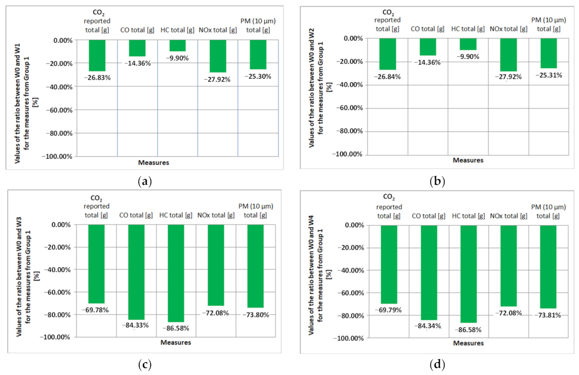
- Group 1—measures related to the total emission of selected harmful substances:
- ○
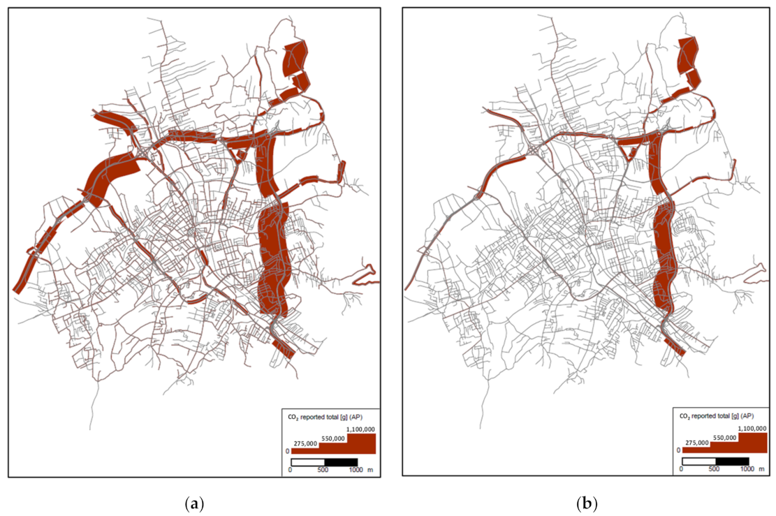
- carbon dioxide (CO2) reported total [g];
- ○
- carbon monoxide (CO) total [g];
- ○
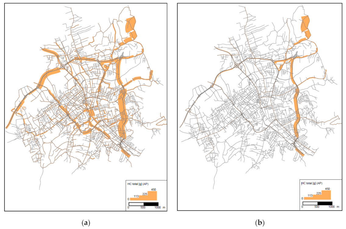
- hydrocarbons (HC) total [g];
- ○
- nitrogen oxides (NOx) total [g];
- ○
- particulate matter (PM) 10 µm total [g].
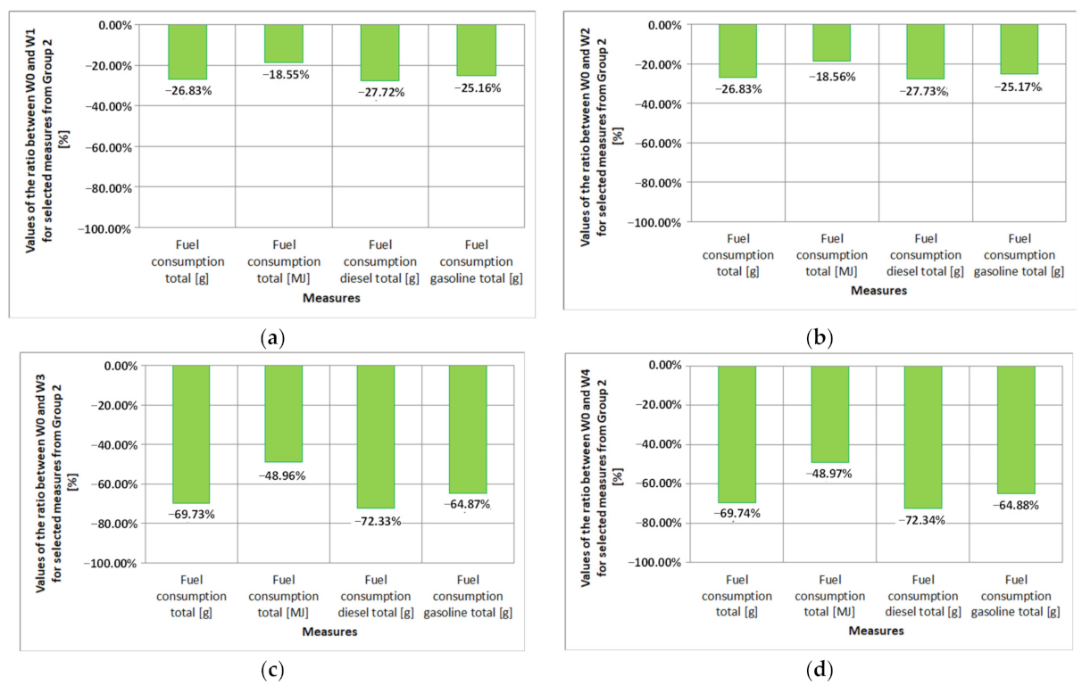
- Group 2—measures related to the consumption of fuels and energy:
- ○
- fuel consumption total [g];
- ○
- fuel consumption total [MJ];
- ○
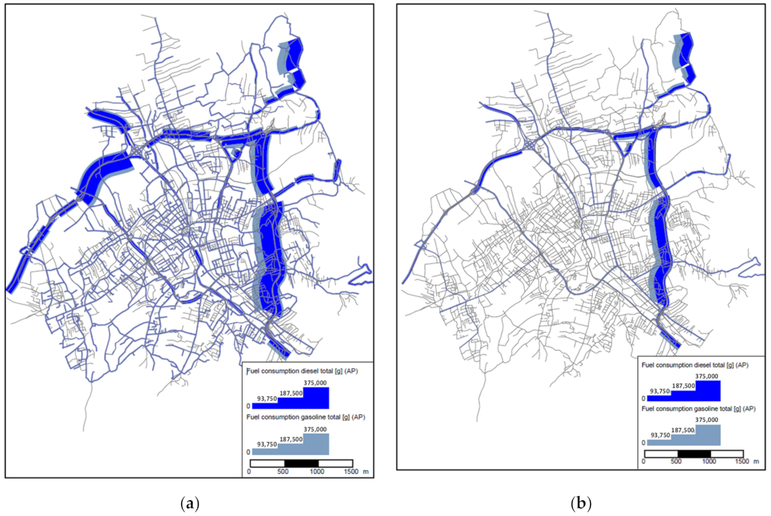
- fuel consumption diesel total [g];
- ○
- fuel consumption gasoline total [g];
- ○
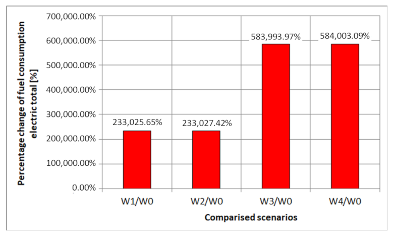
- fuel consumption electric total [MJ].
- Group 3—measures related to the traffic parameters:
- ○
- total time spent in network [h];
- ○
- average speed in network [km/h].
4. Case Study
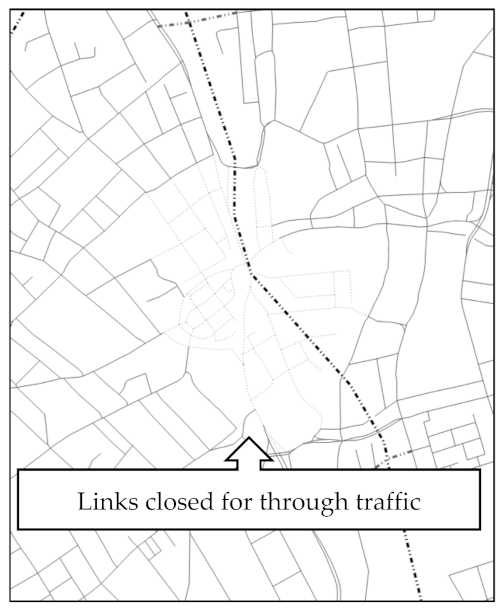
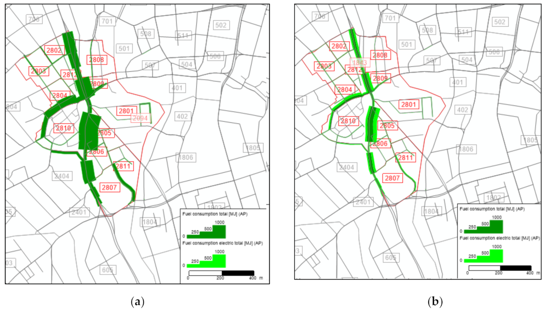
4.1. Research Area
- links for trucks, truck trailers, articulated trucks in through traffic;
- central areas of the city.
4.2. Assumptions Concerning the Scenarios
- Scenario W1:
- ○
- entry of high-emission vehicles from outside the analysed area is not allowed;
- ○
- through traffic is not allowed in the central areas of the city.
- Scenario W2:
- ○
- entry of high-emission vehicles from outside the analysed area is not allowed;
- ○
- through traffic is allowed.
- Scenario W3:
- ○
- entry of all high-emission vehicles is not allowed;
- ○
- through traffic is not allowed in the central areas of the city.
- Scenario W4:
- ○
- entry of all high-emission vehicles is not allowed;
- ○
- through traffic is allowed.
- types of traffic, i.e., inbound, outbound and through traffic;
- types of fleet composition (according to the specification in Table 2).
4.3. Results of the Analyses for the Whole City (Global Scale)
4.4. Results of the Analyses for the Central Areas of the City (Local Scale)
5. Discussion
5.1. General Comments and Observations
5.2. Discussion of Citywide Analyses
5.3. Discussion of the Analyses Carried out for the Central City Area
6. Conclusions
Author Contributions
Funding
Acknowledgments
Conflicts of Interest
References
- Karoń, G.; Żochowska, R. Problems of Quality of Public Transportation Systems in Smart Cities—Smoothness and Disruptions in Urban Traffic. In Modelling of the Interaction of the Different Vehicles and Various Transport Modes, Lecture Notes in Intelligent Transportation and Infrastructure; Sładkowski, A., Ed.; Springer: Berlin/Heidelberg, Germany, 2020. [Google Scholar]
- Cieśla, M.; Sobota, A.; Jacyna, M. Multi-Criteria decision making process in metropolitan transport means selection based on the sharing mobility idea. Sustainability 2020, 12, 7231. [Google Scholar] [CrossRef]
- Cartenì, A.; Henke, I.; Molitierno, C.; Di Francesco, L. Strong Sustainability in Public Transport Policies: An e-Mobility Bus Fleet Application in Sorrento Peninsula (Italy). Sustainability 2020, 12, 7033. [Google Scholar] [CrossRef]
- Cartenì, A. A cost-benefit analysis based on the carbon footprint derived from plug-in hybrid electric buses for urban public transport services. WSEAS Trans. Environ. Dev. 2018, 14, 125–135. [Google Scholar]
- Karoń, G.; Żochowska, R. Modelling of Expected Traffic Smoothness in Urban Transportation Systems for ITS Solutions. Arch. Transp. 2015, 33, 33–45. [Google Scholar] [CrossRef]
- Quak, H. Sustainability of Urban Freight Transport: Retail Distribution and Local Regulations in Cities (No. EPS-2008-124-LIS); Erasmus Research Institute of Management (ERIM): Rotterdam, The Netherlands, 2008. [Google Scholar]
- Banister, D. Unsustainable Transport: City Transport in the New Century; Taylor & Francis: Abingdon, UK, 2005. [Google Scholar]
- Rietveld, P.; Bruinsma, F. Is Transport Infrastructure Effective? Transport Infrastructure and Accessibility: Impacts on the Space Economy; Springer Science & Business Media: Berlin/Heidelberg, Germany, 2012. [Google Scholar]
- Jacyna, M.; Wasiak, M.; Lewczuk, K.; Chamier-Gliszczyński, N.; Dąbrowski, T. Decision problems in developing proecological transport system. Annu. Set Environ. Prot. 2018, 20, 1007–1025. [Google Scholar]
- Figliozzi, M.A. The impacts of congestion on time-definitive urban freight distribution networks CO2 emission levels: Results from a case study in Portland, Oregon. Transp. Res. Part C Emerg. Technol. 2011, 19, 766–778. [Google Scholar] [CrossRef]
- Szczepański, E.; Jacyna, M. An approach to optimize the cargo distribution in urban areas. Logist. Transp. 2013, 17, 53–62. [Google Scholar]
- Jacyna, M. The role of the cargo consolidation center in urban logistics system. Int. J. Sustain. Dev. Plan. 2013, 8, 100–113. [Google Scholar] [CrossRef]
- Wasiak, M.; Jacyna, M.; Lewczuk, K.; Szczepański, E. The method for evaluation of efficiency of the concept of centrally managed distribution in cities. Transport 2017, 32, 348–357. [Google Scholar] [CrossRef] [Green Version]
- Tang, U.W.; Wang, Z.S. Influences of urban forms on traffic-induced noise and air pollution: Results from a modelling system. Environ. Model. Softw. 2007, 22, 1750–1764. [Google Scholar] [CrossRef]
- Fuks, K.; Moebus, S.; Hertel, S.; Viehmann, A.; Nonnemacher, M.; Dragano, N.; Möhlenkamp, S.; Jakobs, H.; Kessler, C.; Erbel, R.; et al. Long-term urban particulate air pollution, traffic noise, and arterial blood pressure. Environ. Health Perspect. 2007, 119, 1706–1711. [Google Scholar] [CrossRef] [Green Version]
- Jacyna, M.; Wasiak, M. Costs of road transport depending on the type of vehicles. Combust. Engines 2015, 162, 85–90. [Google Scholar]
- Wasiak, M.; Jacyna, M. Model of transport costs in the function of the road vehicles structure. In Proceedings of the 19th International Conference Transport Means 2015, Kaunas, Lithuania, 22–23 October 2015; Proceedings/Kersys Robertas (red.); Transport Means: 2015; Publishing House “Technologija”. pp. 669–677. [Google Scholar]
- Visser, J.; Van Binsbergen, A.; Nemoto, T. Urban freight transport policy and planning. In City Logistics I; Wiley-ISTE: London, UK, 1999; pp. 39–70. [Google Scholar]
- Behrends, S.; Lindholm, M.; Woxenius, J. The impact of urban freight transport: A definition of sustainability from an actor’s perspective. Transp. Plan. Technol. 2008, 31, 693–713. [Google Scholar] [CrossRef] [Green Version]
- Jacyna, M.; Wasiak, M.; Lewczuk, K.; Kłodawski, M. Simulation model of transport system of Poland as a tool for developing sustainable transport. Arch. Transp. 2014, 31, 23–35. [Google Scholar] [CrossRef]
- Schreyer, C.; Schneider, C.; Maibach, M.; Rothengatter, W.; Doll, C.; Schmedding, D. External Costs of Transport—Update Study; Final Report; IWW Uniwersitaet Karlsruhe, INFRAS: Zurich, Switzerland; Karlsruhe, Germany, 2004. [Google Scholar]
- Żochowska, R.; Karoń, G. ITS services packages as a tool for managing traffic congestion in cities. In Intelligent Transportation Systems—Problems and Perspectives; Sładkowski, A., Pamuła, W., Eds.; Series: “Studies in Systems Decision and Control”; Springer: Berlin/Heidelberg, Germany, 2016; Volume 32, pp. 81–103. [Google Scholar] [CrossRef]
- De Palma, A.; Lindsey, R. Traffic congestion pricing methodologies and technologies. Transp. Res. Part C Emerg. Technol. 2011, 19, 1377–1399. [Google Scholar] [CrossRef]
- Levy, J.I.; Buonocore, J.J.; Von Stackelberg, K. Evaluation of the public health impacts of traffic congestion: A health risk assessment. Environ. Health 2010, 9, 1–12. [Google Scholar] [CrossRef] [Green Version]
- Stokols, D.; Novaco, R.W.; Stokols, J.; Campbell, J. Traffic congestion, Type A behavior, and stress. J. Appl. Psychol. 1978, 63, 467. [Google Scholar] [CrossRef]
- Luo, Q.; Juan, Z.; SUN, B.; Jia, H. Method research on measuring the external costs of urban traffic congestion. J. Transp. Syst. Eng. Inf. Technol. 2007, 7, 9–12. [Google Scholar] [CrossRef]
- Jacyna-Gołda, I.; Żak, J.; Gołębiowski, P. Models of traffic flow distribution for various scenarios of the development of proecological transport system. Arch. Transp. 2014, 4, 17–28. [Google Scholar] [CrossRef]
- Vaitiekūnas, P.; Banaitytė, R. Modeling of motor transport exhaust pollutant dispersion. J. Environ. Eng. Landsc. Manag. 2007, 14, 39–46. [Google Scholar] [CrossRef] [Green Version]
- Jacyna, M.; Lewczuk, K.; Szczepański, E.; Gołębiowski, P.; Jachimowski, R.; Kłodawski, M.; Pyza, D.; Sivets, O.; Wasiak, M.; Zak, J.; et al. Effectiveness of national transport system according to costs of emission of pollutants. In Safety and Reliability: Methodology and Applications; Nowakowski, T., Ed.; CRC Press: Boca Raton, FL, USA, 2015; pp. 559–567. [Google Scholar]
- Galilea, P.; de Dios Ortuzar, J. Valuing noise level reductions in a residential location context. Transp. Res. Part D Transp. Environ. 2005, 10, 305–322. [Google Scholar] [CrossRef] [Green Version]
- Jakovljevic, B.; Paunovic, K.; Belojevic, G. Road-traffic noise and factors influencing noise annoyance in an urban population. Environ. Int. 2009, 35, 552–556. [Google Scholar] [CrossRef] [PubMed]
- Filippone, A. Aircraft noise prediction. Prog. Aerosp. Sci. 2014, 68, 27–63. [Google Scholar] [CrossRef]
- Den Boer, E.; Schroten, A. Traffic noise reduction in Europe. CE Delft 2007, 14, 2057–2068. [Google Scholar]
- Monetisation of the Health Impact due to Traffic Noise; Swiss Agency for the Environment, Forests and Landscape: Bern, Switzerland, 2003.
- Bickel, P.; Friedrich, R.; Burgess, A.; Fagiani, P.; Hunt, A.; De Jong, G.; Laird, J.; Lieb, C.; Lindberg, G.; Mackie, P.; et al. Proposal for Harmonised Guidelines; Deliverable D5 of HEATCO Project; IER—University of Stuttgart: Stuttgart, Germany, 2006. [Google Scholar]
- Korzhenevych, A.; Dehnen, N.; Bröcker, J.; Holtkamp, M.; Meier, H.; Gibson, G.; Varma, A.; Cox, V. Update of the Handbook on External Costs of Transport. In Final Report: Report for the European Commission: DG MOVE Ricardo-AEA/R/ED57769 Issue Number 18 January 2014; 2014; Available online: https://ec.europa.eu/transport/sites/transport/files/handbook_on_external_costs_of_transport_2014_0.pdf (accessed on 10 February 2021).
- Proost, S. TREMOVE 2 Service Contract for the Further Development and Application of the TREMOVE Transport Model—Lot 3: Final Report Part 2: Description of the Baseline; European Commission, Directorate General of the Environment: Brussels, Belgium, 2006. [Google Scholar]
- Merkisz, J.; Jacyna, M.; Merkisz-Guranowska, A.; Pielecha, J. The parameters of passenger cars engine in terms of real drive emission test. Arch. Transp. 2014, 32, 43–50. [Google Scholar] [CrossRef] [Green Version]
- Chamier-Gliszczyński, N.; Bohdal, T. Mobility in Urban Areas in Environment Protection. Rocz. Ochr. Środowiska 2016, 18, 387–399. [Google Scholar]
- Jacyna, M.; Wasiak, M. The study of transport impact on the environment with regard to sustainable development. Vibroeng. Procedia 2017, 13, 285–289. [Google Scholar] [CrossRef] [Green Version]
- Jacyna, M.; Wasiak, M.; Lewczuk, K.; Karoń, G. Noise and environmental pollution from transport: Decisive problems in developing ecologically efficient transport systems. J. Vibroeng. 2017, 19, 5639–5655. [Google Scholar] [CrossRef]
- Wasiak, M.; Niculescu, A.I.; Kowalski, M. A generalized method for assessing emissions from road and air transport on the example of Warsaw Chopin Airport. Arch. Civ. Eng. 2020, 66, 399–419. [Google Scholar]
- Available online: www.ptvgroup.com (accessed on 10 February 2021).
- Shafiei, E.; Leaver, J.; Davidsdottir, B. Cost-effectiveness analysis of inducing green vehicles to achieve deep reductions in greenhouse gas emissions in New Zealand. J. Clean. Prod. 2017, 150, 339–351. [Google Scholar] [CrossRef]
- Shi, F.; Xu, G.M.; Liu, B.; Huang, H. Optimization method of alternate traffic restriction scheme based on elastic demand and mode choice behaviour. Transp. Res. Part C 2014, 39, 36–52. [Google Scholar] [CrossRef]
- Kholod, N.; Evans, M.; Gusev, E.; Yu, S.; Malyshev, V.; Tretyakova, S.; Barinov, A. A methodology for calculating transport emissions in cities with limited traffic data: Case study of diesel particulates and black carbon emissions in Murmansk. Sci. Total. Environ. 2016, 547, 305–313. [Google Scholar] [CrossRef] [Green Version]
- Lu, J.; Li, B.; Li, H.; Al-Barakani, A. Expansion of city scale, traffic modes, traffic congestion, and air pollution. Cities 2021, 108, 102974. [Google Scholar] [CrossRef]
- Wang, L.; Xu, J.; Qin, P. Will a driving restriction policy reduce car trips?—The case study of Beijing, China. Transp. Res. Part A 2014, 67, 279–290. [Google Scholar] [CrossRef]
- Gundlach, A.; Ehrlinspiel, M.; Kirsch, S.; Koschker, A.; Sagebiel, J. Investigating people’s preferences for car-free city centers: A discrete choice experiment. Transp. Res. Part D 2018, 63, 677–688. [Google Scholar] [CrossRef]
- Schubert, T.; Dziekan, K.; Kiso, C. Tomorrow’s Cities: Towards livable cities with lower car densities. Transp. Res. Procedia 2019, 41, 260–263. [Google Scholar] [CrossRef]
- Pasha, A.; Rastogi, R.; Mir, M.S. Impact of Car Restrictive Policies: A Case Study of Srinagar City in J&K State India. Transp. Res. Procedia 2020, 48, 2690–2705. [Google Scholar]
- Nosal, K.; Starowicz, W. Evaluation of influence of mobility management instruments implemented in separated areas of the city on the changes in modal split. Arch. Transp. 2015, 35, 41–52. [Google Scholar] [CrossRef]
- Bagheri, M.; Ghafourian, H.; Kashefiolasl, M.; Pour, M.T.S.; Rabbani, M. Travel management optimization based on air pollution condition using Markov decision process and genetic algorithm (case study: Shiraz city). Arch. Transp. 2020, 53, 89–102. [Google Scholar] [CrossRef]
- Jacyna, M.; Merkisz, J. Proecological approach to modelling traffic organization in national transport system. Arch. Transp. 2014, 30, 31–41. [Google Scholar] [CrossRef] [Green Version]
- Notter, B.; Keller, M.; Althaus, H.J.; Cox, B. HBEFA, Handbook Emission Factors for Road Transport 4.1, Quick Reference; Bern, Germany; 28 June 2019; Available online: https://www.hbefa.net/e/help/HBEFA41_help_en.pdf (accessed on 10 February 2021).


| Instrument Name | Instrument Type | Efficiency | Cost-Effectiveness Index * |
|---|---|---|---|
| Communication noise | |||
| New brake systems for railway vehicles | Technical | High | 1 |
| Design changes of engines | Technical | Low | 2 |
| Speed limits | Command and control | Average | 3 |
| Tires with reduced noise levels | Technical | Low | 4 |
| Soundproof walls/soundproof screens | Infrastructure | High | 5 |
| Air pollution | |||
| Buses and other vehicles with alternative drive (low and zero emission) | Technical | Low | 1 |
| EURO emission standards | Command and control | High | 2 |
| Emission-related tolls Fuel tax | Economic | High | 3 |
| City parking policy (availability, prices) | Economic/infrastructure | Average | 4 |
| Tariff policy in urban public transport | Economic | Average | 5 |
| Traffic bans in the city (low and zero emission zones) | Command and control | High | 6 |
| Speed limits | Command and control | Average | 7 |
| Climate changes | |||
| Economic driving courses | Organisational/institutional | Average | 1 |
| Kyoto Mechanism (Emissions Trading, Clean Development Mechanisms) | Economic | High | 2 |
| Fuel tax | Economic | High | 3 |
| Renewable energy sources for electricity production (railways, electric vehicles) | Technical | High | 4 |
| Buses and other vehicles with alternative drive (low and zero emission) | Technical | High | 5 |
| Tolling on vehicles with high fuel consumption and CO2 emissions or fuel consumption (i.e., low fuel efficiency) and rebates for low CO2 emissions or fuel-efficient vehicles. | Economic | Low | 6 |
| EURO standards for exhaust emissions and alternative fuels | Command and control | Average | 7 |
| Speed limits | Command and control | Average | 8 |
| Fleet Composition | Type of Vehicles | Types of Fleet Composition |
|---|---|---|
| Urban | passenger car | A |
| light commercial vehicle | B | |
| mix (trucks, truck trailers, articulated trucks) | C | |
| Average | passenger car | D |
| light commercial vehicle | E | |
| mix (trucks, truck trailers, articulated trucks) | F | |
| Motorway | passenger car | G |
| light commercial vehicle | H | |
| mix (trucks, truck trailers, articulated trucks) | I | |
| Electric | passenger car | J |
| light commercial vehicle | K | |
| mix (trucks, truck trailers, articulated trucks) | L |
| Type of Traffic | Volume of Car Traffic [E/h] | Share of Car Traffic [%] |
|---|---|---|
| Inbound traffic | 14,403 | 47.79 |
| Outbound traffic (the city is the origin of the trip) | 5698 | 18.91 |
| Outbound traffic (the city is the destination of the trip) | 8159 | 27.07 |
| Through traffic | 1880 | 6.24 |
| TOTAL | 30,140 | 100.00 |
| Type of Traffic | Scenario W0 | Scenario W1 | Scenario W2 | Scenario W3 | Scenario W4 |
|---|---|---|---|---|---|
| Inbound traffic | A, B, C | A, B, C | A, B, C | J, K, L | J, K, L |
| Outbound traffic (the city is the origin of the trip) | A, B, C | A, B, C | A, B, C | J, K, L | J, K, L |
| Outbound traffic (the city is the destination of the trip) | D, E, F | J, K, L | J, K, L | J, K, L | J, K, L |
| Through traffic | G, H, I | G, H, I (without central areas of the city) | G, H, I | G, H, I (without central areas of the city) | G, H, I |
| Measure of Assessment | Scenario W0 | Scenario W1 | Scenario W2 | Scenario W3 | Scenario W4 |
|---|---|---|---|---|---|
| Group 1 | |||||
| CO2 reported total [g] | 42,343,255.82 | 30,984,001.26 | 30,980,307.60 | 12,797,176.89 | 12,793,777.41 |
| CO total [g] | 184,107.10 | 157,678.34 | 157,676.72 | 28,845.66 | 28,837.32 |
| HC total [g] | 29,186.26 | 26,296.08 | 26,295.47 | 3917.83 | 3917.20 |
| NOx total [g] | 194,904.37 | 140,494.09 | 140,482.04 | 54,422.58 | 54,408.70 |
| PM (10 µm) total [g] | 7991.16 | 5969.17 | 5968.66 | 2093.45 | 2092.81 |
| Group 2 | |||||
| Fuel consumption total [g] | 14,580,702.09 | 10,669,279.59 | 10,668,006.20 | 4,413,042.97 | 4,411,871.06 |
| Fuel consumption total [MJ] | 616,895.76 | 502,461.61 | 502,408.14 | 314,856.75 | 314,809.19 |
| Fuel consumption diesel total [g] | 9,504,016.51 | 6,869,764.36 | 6,868,988.59 | 2,629,596.30 | 2,628,879.40 |
| Fuel consumption gasoline total [g] | 5,076,530.12 | 3,799,396.56 | 3,798,898.96 | 1,783,358.59 | 1,782,903.60 |
| Fuel consumption electric total [MJ] | 21.96 | 51,182.74 | 51,183.13 | 128,237.83 | 128,239.83 |
| Group 3 | |||||
| Total time spend in network [h] | 108.34 | 108.16 | 108.34 | 108.16 | 108.34 |
| Average speed in network [km/h] | 33.03 | 33.03 | 33.03 | 33.03 | 33.03 |
| Measure of Assessment | Scenario W1 | Scenario W2 | Scenario W3 | Scenario W4 |
|---|---|---|---|---|
| Group 1 | ||||
| CO2 reported total [g] | 4 | 3 | 2 | 1 |
| CO total [g] | 4 | 3 | 2 | 1 |
| HC total [g] | 4 | 3 | 2 | 1 |
| NOx total [g] | 4 | 3 | 2 | 1 |
| PM (10 µm) total [g] | 4 | 3 | 2 | 1 |
| Group 2 | ||||
| Fuel consumption total [g] | 4 | 3 | 2 | 1 |
| Fuel consumption total [MJ] | 4 | 3 | 2 | 1 |
| Fuel consumption diesel total [g] | 4 | 3 | 2 | 1 |
| Fuel consumption gasoline total [g] | 4 | 3 | 2 | 1 |
| Fuel consumption electric total [MJ] | 1 | 2 | 3 | 4 |
| Group 3 | ||||
| Total time spend in network [h] | 1 | 2 | 1 | 2 |
| Average speed in network [km/h] | 1 | 2 | 1 | 2 |
| Measure of Assessment | Scenario W0 | Scenario W1 | Scenario W2 | Scenario W3 | Scenario W4 |
|---|---|---|---|---|---|
| Group 1 | |||||
| CO2 reported total [g] | 858,504.30 | 670,728.44 | 673,202.79 | 1033.93 | 3508.28 |
| CO total [g] | 5309.83 | 4922.72 | 4927.67 | 2.60 | 7.55 |
| HC total [g] | 943.74 | 898.60 | 899.10 | 0.24 | 0.75 |
| NOx total [g] | 3737.12 | 2915.01 | 2924.82 | 4.49 | 14.30 |
| PM (10 µm) total [g] | 167.95 | 135.95 | 136.32 | 0.18 | 0.55 |
| Group 2 | |||||
| Fuel consumption total [g] | 295,550.57 | 230,849.60 | 231,702.57 | 356.37 | 1209.34 |
| Fuel consumption total [MJ] | 12,498.38 | 10,549.47 | 10,585.55 | 3487.12 | 3523.21 |
| Fuel consumption diesel total [g] | 189,812.73 | 148,453.24 | 148,976.21 | 221.43 | 744.41 |
| Fuel consumption gasoline total [g] | 105,736.01 | 82,395.15 | 82,725.12 | 134.93 | 464.91 |
| Fuel consumption electric total [MJ] | 21.96 | 789.44 | 789.44 | 3472.05 | 3472.05 |
| Group 3 | |||||
| Total time spend in network [h] | 1.08 | 0.93 | 1.08 | 0.93 | 1.08 |
| Average speed in network [km/h] | 25.03 | 25.05 | 25.03 | 25.05 | 25.03 |
| Measure of Assessment | Scenario W1 | Scenario W2 | Scenario W3 | Scenario W4 |
|---|---|---|---|---|
| Group 1 | ||||
| CO2 reported total [g] | 3 | 4 | 1 | 2 |
| CO total [g] | 3 | 4 | 1 | 2 |
| HC total [g] | 3 | 4 | 1 | 2 |
| NOx total [g] | 3 | 4 | 1 | 2 |
| PM (10 µm) total [g] | 1 | 4 | 1 | 2 |
| Group 2 | ||||
| Fuel consumption total [g] | 3 | 4 | 1 | 2 |
| Fuel consumption total [MJ] | 3 | 4 | 1 | 2 |
| Fuel consumption diesel total [g] | 3 | 4 | 1 | 2 |
| Fuel consumption gasoline total [g] | 3 | 4 | 1 | 2 |
| Fuel consumption electric total [MJ] | 2 | 2 | 1 | 1 |
| Group 3 | ||||
| Total time spend in network [h] | 1 | 2 | 1 | 2 |
| Average speed in network [km/h] | 2 | 1 | 2 | 1 |
Publisher’s Note: MDPI stays neutral with regard to jurisdictional claims in published maps and institutional affiliations. |
© 2021 by the authors. Licensee MDPI, Basel, Switzerland. This article is an open access article distributed under the terms and conditions of the Creative Commons Attribution (CC BY) license (https://creativecommons.org/licenses/by/4.0/).
Share and Cite
Jacyna, M.; Żochowska, R.; Sobota, A.; Wasiak, M. Scenario Analyses of Exhaust Emissions Reduction through the Introduction of Electric Vehicles into the City. Energies 2021, 14, 2030. https://doi.org/10.3390/en14072030
Jacyna M, Żochowska R, Sobota A, Wasiak M. Scenario Analyses of Exhaust Emissions Reduction through the Introduction of Electric Vehicles into the City. Energies. 2021; 14(7):2030. https://doi.org/10.3390/en14072030
Chicago/Turabian StyleJacyna, Marianna, Renata Żochowska, Aleksander Sobota, and Mariusz Wasiak. 2021. "Scenario Analyses of Exhaust Emissions Reduction through the Introduction of Electric Vehicles into the City" Energies 14, no. 7: 2030. https://doi.org/10.3390/en14072030