Time-Dependent Heat Transfer Calculations with Trefftz and Picard Methods for Flow Boiling in a Mini-Channel Heat Sink

Abstract

The intensification of heat transfer using two-phase boiling flow in mini-channels is widely used to dissipate the high heat fluxes in miniaturized electronic devices. However, the process itself is not fully recognized and still requires experimental studies and developing computation methods appropriate for them. The main aim of this work was the mathematical modeling of time-dependent heat transfer process in FC-72 flow boiling in a mini-channel heat sink with five parallel mini-channels of 1 mm depth. Channels have an asymmetrically heated wall while its outer temperature was measured by infrared thermography. The opposite wall of the mini-channels was transparent, helping to record flow patterns due to a high-speed digital camera. The objective of the numerical calculations was to determine the heat transfer coefficient on the wall-fluid contact surface from the Robin boundary condition. The problem was solved using methods based on the Trefftz-type functions. Three mathematical methods were applied in calculations: the FEM with Trefftz type basis functions, the Classical Trefftz Method, and the Hybrid Picard-Trefftz Method. The results were compared with the values of the heat transfer coefficient obtained from theoretical correlations from the literature.

1. Introduction

There has been an increased interest in mini-channel heat sinks for over 20 years. Heat sinks can be categorized into micro-channels, mini-channels, and conventional ones. According to Kandlikar classification, the channels of hydraulic diameter in the range from 200 μm to 3 mm are named as mini-channels. Change of phase during flow has drawn considerable interest in the engineering community due to the use of latent vaporization heat. The use of boiling phenomena is one of the ways of intensification of heat transfer. Nowadays, there are increasing interests on heat exchangers with mini- or micro-channels due to these advantages mentioned above, resulting in high process efficiency and compactness of technological solutions. Several recent applications of mini-channel heat sinks cover the computer and IT industry, miniature refrigeration systems, domestic micro ORC, and cooling of PEM fuel cells. It is worth mentioning that miniaturization has become a requirement in the design of energy and process systems. The results of the scale reduction of the channels for heat transfer have not been recognized yet; therefore, further experimental and theoretical studies are required.

State-of-the-art focused on heat transfer in small confined spaces was presented in [1]. Physical phenomena accompanying flow boiling, such as flow maldistributions and other instabilities of pressure and temperature, are often also the subject of researchers’ concern [2,3,4]. It is worth mentioning that lots of work deal also with condensation heat transfer [5,6] or pool boiling [7,8,9]. Heat transfer during fluid flow in mini gaps is the main interest of various technological aspects such as seals [10,11]. A lot of previous works of the authors of this publication focused on flow boiling heat transfer. They are mostly concerned with experimental studies and theoretical analyzes based on steady state research on the test section with longer mini-channels as presented here, often with an enhanced heated surface [12,13], while some of these publications deal with time-dependent experiments [14,15]. A problem concerning a narrow gap was modeled in annular geometry and successfully solved [16]. Furthermore, the commercial program ADINA was applied in numerical computations [1]. The first attempts of using ANSYS program were also done [17]. ANSYS CFX and ANSYS Fluent are widely used as the most common numerical methods in computational fluid dynamics [18].

The technological advances of today are accompanied by the rapid development of numerical methods. Mathematical modeling makes it possible to analyze physical phenomena which are frequently described by linear and non-linear differential equations. Ref. [19] provides a review of previous studies of steady-state flow boiling in micro-channels, with a focus on the computational work while [1] presents a comprehensive overview of experimental investigations on flow boiling in mini-channels. A characteristic feature of many engineering problems is the high sensitivity of the solutions to the uncertainties of the input data, especially in inverse problems, where small changes in the inputs can result in very large changes in the outputs. Hence, these problems are called ill-posed problems [20] due to the instability of their solutions. This difficulty may be exacerbated when we consider two or more subsequent time-dependent inverse problems. In such a case, even advanced commercial programs could fail. Hence, there appears a need for developing stable methods (multigrid methods or grid-free methods) for solving inverse engineering problems, including coupled time-dependent inverse problems. The methods using the Trefftz-type functions (T-functions) meet the aforementioned requirements and the results already obtained support this view [21,22,23,24].

The literature on the subject reports numerous applications of the Trefftz method. One such method is the grid-free classical Trefftz method [25]. Many authors count it among the analytical-numerical methods, as it allows to find a solution that exactly satisfies the governing equation, whereas the set initial and boundary conditions are approximately satisfied. An approximation of the solution is the linear combination of the Trefftz functions, the coefficients of which are selected so that the approximation meets a specified criterion. It should be pointed out that Trefftz functions are linearly independent and form a complete system. A detailed description of the method and its broad scope of applications was discussed in [21,26,27,28,29]. The types and modifications of the Trefftz method can be found in [30,31]. Many researchers use T-functions for various problems involving heat transfer [22,32,33]. For more complex problems, the analyzed area was usually divided into elements, as in [14,34,35,36,37], where the Trefftz functions served as basis functions in FEM.

The Trefftz method has also found application in finding solutions of non-linear equations by combining it with other methods. The combination of the Trefftz method and homotopy is reported in [32,38]. The combined methods were used to solve non-linear problems, such as potential problems [39]. Non-linear problems can be solved by combining the Trefftz function with Picard’s iteration. In such approach, each iteration step yields a linear equation, which is solved using the Trefftz method, as shown in [23], whose authors successfully dealt with direct and inverse non-linear heat conduction problems. Combining the Trefftz method with Picard’s iteration is an efficient tool for determining some physical coefficients, e.g., the heat transfer coefficient [40] and the parameters of the microjet cooling process [41].

Picard’s method of successive approximations can also be used to find the non-differential solution to the heat problem in fractal media with local fractional derivative. This method was applied in [42] to demonstrate solving the local fractional heat conduction equations.

A detailed history of the evolution of Picard’s iteration can be found in [43]. It is known as the method of successive approximations. A number of researchers then reported using this method for nth-order linear differential equations, but the most comprehensive form of the method was developed by Emile Picard [44]. The convergence analysis of the method was presented in [45]. The first researchers to use the iteration method were Clenshaw and Norton [46], who proposed combining Chebyshev series with Picard’s iteration.

The present paper proposes a mathematical model of time-dependent heat transfer in flow boiling of the FC-72 refrigerant in a rectangular mini-channel with an asymmetrically heated wall. The formulated model concerns a laminar flow with void fraction not exceeding 10% and constitutes the starting point for a mathematical description of two-phase flow with higher values of void fraction. In the presented approach, it was assumed that the heater temperature distribution was described by the Fourier equation, whereas in the flowing fluid by the energy equation with a known profile of one component of the fluid velocity (the other velocity components were assumed equal to zero).

A novelty of this publication is the formulation of a time-dependent mathematical model of heat transfer in a mini-channel and solving it using three methods based on the Trefftz functions: (i) the FEM with the Trefftz-type basis functions (FEMT), (ii) the Classical Trefftz Method (CTM), and (iii) the Hybrid Picard-Trefftz Method (HPTM). Importantly, the calculations were performed using the experimental time-dependent data. Two types of T- functions were used in the numerical calculations: time-independent functions for the Laplace and energy equation [47] and time-dependent T-functions for the Fourier [27] and for the Fourier-Kirchhoff equations (Maciejewska and Piasecka, 2019). Depending on the experimental results, the fluid velocity, void fraction, and the negative heat sources were taken into account in both energy equations. The system of partial differential equations was solved subject to a set of initial and boundary conditions only partially known. In addition, for the validation of our own results, theoretical correlations from the literature were used, to which own experimental data were introduced.

2. Experiment

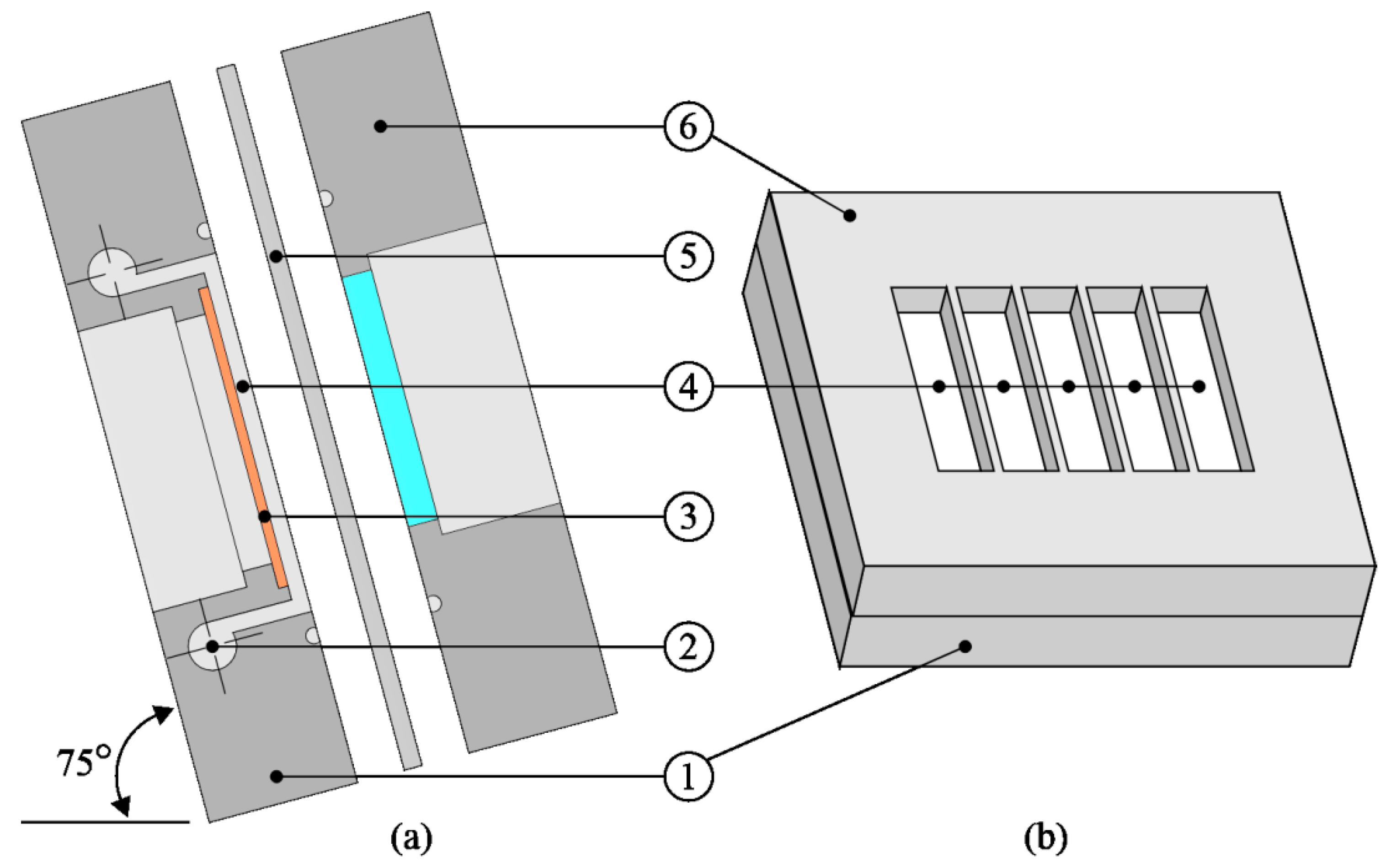
2.1. Experimental Apparatus

The experimental apparatus is shown in Figure 1. During the experiment, Fluorinert FC-72 is recirculated in the flow loop. This loop consists of the following elements: a test section with mini-channels (1), a recirculating pump (2), a compensating tank (3), a heat exchanger (4), a filter (5), a flow meter (6) and a deaerator (7).

The data and image acquisition system, designed to collect the measurement data, includes: an infrared camera (9) and a high-speed digital camera (10). Infrared thermography is applied for measuring of the temperature distribution on the mini-channel heated wall. Simultaneously, a high-speed camera helps to identify flow structures in mini-channels during fluid flow. The PC computer (8) and two data acquisition stations complete this system. The supply and control system contains a power supply unit.

The test section is depicted in Figure 2. It contains five mini-channels, each 1 mm deep, 6 mm wide, and 38 mm long. The main parts of the test section: a front cover and a channel body are made of aluminum alloy, the internal side walls of the channels are formed by Teflon plate. A plate 0.45 mm thick, made of Haynes-230 alloy, constitutes a common heated wall of the mini-channels. The outer plate surface temperature is recorded by an infrared camera. The temperature is measured from the outer surface of the test section, contacting ambient air. The fluid temperature and pressure are controlled at the inlet and outlet manifolds. During the experiment, the test section was placed at an angle of 75 degrees to the horizontal plane, as shown in Figure 2a.

2.2. Experimental Methodology

During the experiment, the subcooled fluid (Fluorinert FC-72) flows into the mini-channels inlet manifold. Then, the heating power supplied to the heated plate, being the common mini-channel wall, is increased. When it is observed the first bubble departure, it is the evidence of the boiling initiation. Basic experimental thermal and flow parameters are recorded in the selected time interval: from 300 s to 500 s. The temperature of the outer side of the heated wall of the mini-channels is measured by an infrared camera (FLIR, model A655SC). Other experimental parameters are also collected. Simultaneously, two-phase flow images are captured by a high-speed digital camera (JAI, model SP-5000M-CXP2, Denmark/Japan). The visualizations are thoroughly analyzed to better understand the heat transfer process. Based on the saved images during the experiment, after data processing using own software, void fraction in 10 areas along the flow are determined.

2.3. Experimental Parameters and Errors

Basic experimental thermal and flow parameters for the selected time moments of the set as well as the maximum errors are listed in

Table 1. Basic experimental thermal-flow parameters and accuracies.

Temperature of the Heated Plate TH,IR	Temperature of the Fluid at the Inlet Tf,in	Temperature of the Fluid at the Outlet Tf,out	Absolute Error of the Difference in Fluid Temperature	Overpressure at the Inlet	Overpressure at the Outlet	Total Mass Flow Rate	Heat Flux (Density) qw
	Device
IR camera FLIR, A655SC	K-type Thermo- couple, Czaki Thermo- Product, type K 221 b	K-type Thermo- couple, Czaki Thermo- Product, type K 221 b	-	Pressure meter, Endress+ Hauser, Cerabar S PMP71	Pressure meter, Endress+ Hauser, Cerabar S PMP71	Coriolis mass flowmeter, Endress+ Hauser, Proline Promass A 100	-
	Ranges
37.0 ÷ 63.99 °C	23.8 ÷ 25.9 °C	29.1 ÷ 38.3 °C	-	105.9 ÷ 122.5 kPa	97.2 ÷ 113.8 kPa	0.00273 ÷ 0.00280 kg s−1	9.70 ÷ 16.29 kW m−2
	Maximum Error
±1 °C or ±1% in the range 0 ÷ 120 °C, according to the calibration certificate	calibration tolerance 1.5 °C	calibration tolerance 1.5 °C	0.19 °C, according to the additional calibration experiment [48]	±0.05% of reading	±0.05% of reading	±0.1% of reading	3.16%

.

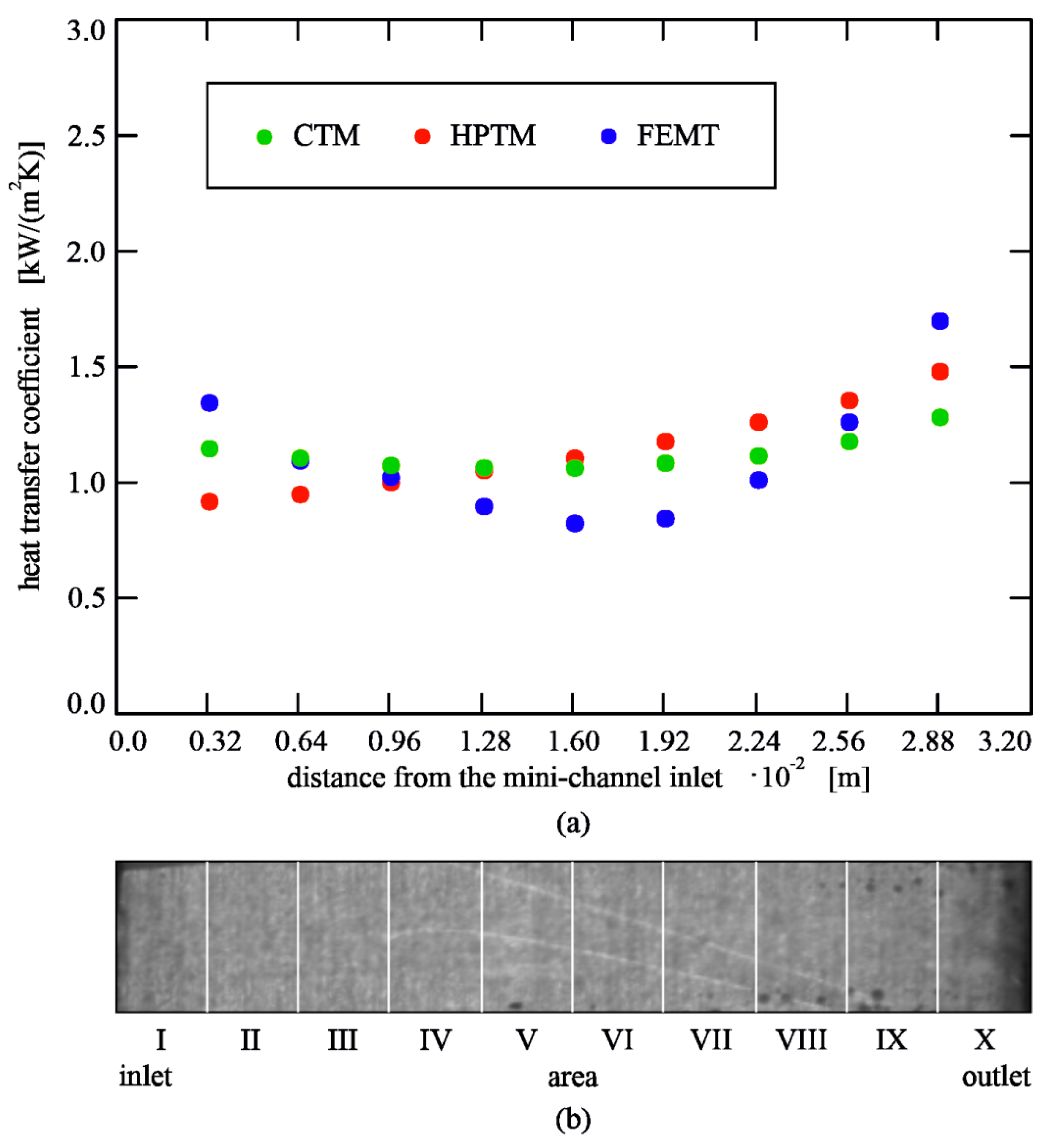
2.4. Raw Experimental Data

The raw data recorded during the experiment are as follows: the temperature distribution on the heated plate, inlet and outlet temperatures and pressures of the working fluid, supplied heat flux (calculated on the basis of current intensity and voltage drop across the heated plate), atmospheric pressure, and mass flow rate. The plate temperature data have to be reduced with the application of the solution to the inverse heat conduction problem. The sought are local values of the heat transfer coefficient in the heated wall-fluid contacting surface. Figure 3 presents the raw temperature data concerning the outer surface of the heated plate, obtained from infrared measurement versus time and the distance from the mini-channel inlet.

3. Void Fraction Determination

Images of two-phase patterns were recorded at a speed of 1 fps with resolution of 360 × 360 pixels. For further processing, only a part of the images corresponding to the central mini-channel were taken. It was necessary to load images to our specialist software environment based on LabVIEW functions. Each digital photo was loaded and analyzed as a binarized image. A set of pixels contained in ten areas evenly divided along each image was taken sequentially. To determine void fraction during the next stage of the program, the number of pixels corresponding to the gas phase were counted and divided by the total number of pixels. For the areas partially filled with vapor, the procedure of closing bubbles was used. It is worth mentioning that two-phase pattern images correspond to the images recorded by an infrared camera, which are taken for further processing and computation. A scheme showing the distribution of areas corresponding to two-phase flow patterns, assumed for void fraction calculation is illustrated in Figure 4. In Figure 5, void fraction obtained from the calculations according to the authors’ own program, versus time and the distance from the mini-channel inlet is presented.

4. Basic Mathematical Model

The mathematical model of heat transfer in a mini-channel suggested in this paper combines and modifies two models: a time-independent model described in [49] and a time-dependent model from [14]. Similarly to [49], two dimensions were taken into account in the approach: one in the direction of the flow (x) and one in the perpendicular direction (y) referring to the thickness of the heated plate and the depth of the mini-channel. The heat transfer process in the heating wall was described using two-dimensional Fourier equation complemented with an appropriate system of boundary conditions [50]:

$$\nabla ·\left({\lambda }_H\nabla T_H\right)={\rho }_H{c}_{pH}\frac{\partial T_H}{\partial t}-q_V\left(t\right) \mathrm{for} \left(x,y\right)\in D_{H }, t> 0,$$

(1)

where $D_H=\left\{\left(x,y\right)\in R^2: 0<x<L, 0<y<{\delta }_H\right\}$. The boundary conditions took into account the time-dependent measurements of the heated plate temperature conducted using infrared thermography, i.e.,:

$$T_H\left(x_m,0,t_n\right)=T_{m,n} \mathrm{for} m=1,2,\dots \mathrm{P}, n=1,2,\dots N.$$

(2)

Additionally, it was assumed that the remaining boundaries of the heated plate, having no contact with the fluid, are isolated.

Assumptions for the flow of the working fluid were similar to [49]:

• fluid flow in the mini-channel is laminar (Reynolds number below 2100) with a constant mass flux density;
• fluid velocity in the mini-channel has one constant component w_x(y) parallel to the heated plate, the other component takes the value of zero;
• the emerging vapor bubbles are an internal negative heat source $\mathsf{\Omega }\left(x,t\right)$ absorbing some part of the energy transferred to the fluid from the heated plate.

With these assumptions, the energy equation written for the liquid phase takes the form:

$$\nabla ·\left({\lambda }_f\nabla T_f\right)={\rho }_f{c}_{p,f}\left(\frac{\partial T_f}{\partial t}+w_x\left(y\right)\frac{\partial T_f}{\partial x}\right)+\mathsf{\Omega }\left(x,t\right) \mathrm{for} \left(x,y\right)\in D_M, t> 0,$$

(3)

where $D_M=\left\{\left(x,y\right)\in R^2: 0<x<L, {\delta }_H<y<{\delta }_H+{\delta }_M\right\}$ and the negative heat source was calculated from the formula [51]:

$$\mathsf{\Omega }\left(x,t\right)=\frac{6{\alpha }_{con}\Delta T\left(t\right)}{d_b\left(t\right)}\phi \left(x,t\right),$$

(4)

and the liquid superheat ΔT(t) was calculated in analogy to [52].

The bubble diameter d_b in subcooled flow boiling was calculated using Tolubinski and Kostanchuk correlation [53,54]:

$$d_b\left(t\right)=min\left(0.0006·exp\left(-\frac{\Delta T\left(t\right)}{45}\right);0.0014\right).$$

(5)

For Equation (3), it was assumed that the fluid temperature at the inlet T_f,in and outlet T_f,out of the mini-channel is known and additionally, the fluid temperature at the contact with the heater surface mainly depends on temperature of the plate, i.e.,:

$$T_f\left(0,y,t\right)=T_{f,in}\left(t\right),$$

(6)

$$T_f\left(L,y,t\right)=T_{f,out}\left(t\right),$$

(7)

$$T_f\left(x,{\delta }_H,t\right)=T_H\left(x,{\delta }_H,t\right).$$

(8)

In further calculations, the boundary conditions have been transformed so that they can be used in the numerical method. This remark applies mainly to the CTM.

5. Solution Methods

The system of energy equations with a set of adopted initial and boundary conditions defines two inverse heat conduction problems (IHCPs) in the heated surface and the flowing fluid. Three methods using the Trefftz functions were applied to solve these inverse problems: the CTM, the HPTM, and the FEMT.

5.1. The Classical Trefftz Method (CTM)

In the CTM, the time-dependent heat conduction problems described by Equations (1) and (3) were reduced to quasi-time independent problems. Additionally, the heater and fluid temperature, T_H,n(x,y) and T_f,n(x,y), respectively, were calculated at discrete times without dividing the domains D_H and D_M into subdomains. This approach allows us to use T-functions (harmonic functions) for the Laplace equation [24,55] and the T-functions for the time-independent energy equation in the fluid in analogy to [47]. As in [47], the heater and fluid temperature were approximated as a sum of a particular solution and a linear combination of the T-functions. Determining the coefficients of a linear combination is described in detail in [24].

5.2. The Hybrid Picard-Trefftz Method (HPTM)

The HPTM was used only to determine the temperature distribution of the fluid and the heater temperature was calculated by CTM. The main idea of Picard’s iterations is a decomposition of a nonlinear operator into a linear and nonlinear part. Equation (3) can be rewritten as:

$${\nabla }^2{T}_f+N{T}_f=\frac{\mathsf{\Omega }\left(x,t\right)}{{\lambda }_f}\mathrm{for} \left(x,y\right)\in D_M, t> 0,$$

(9)

where $N=-\frac{{\rho }_f{c}_{p,f}}{{\lambda }_f}\left(\frac{\partial }{\partial t}+w_x\left(y\right)\frac{\partial }{\partial x}\right)$ denotes a differential operator.

Next, Picard’s iterations method can be used to solve Equation (9) and for k = 2,3,... it gives the following equations to be solved:

$${\nabla }^2{T}_f^{\left(k\right)}=-N{T}_f^{\left(k-1\right)}+\frac{\mathsf{\Omega }\left(x,t\right)}{{\lambda }_f}\mathrm{for} \left(x,y\right)\in D_M, t> 0,$$

(10)

with the initial equation (for k = 1) in the form:

$${\nabla }^2{T}_f^{\left(1\right)}=\frac{\mathsf{\Omega }\left(x,t\right)}{{\lambda }_f}\mathrm{for} \left(x,y\right)\in D_M, t> 0.$$

(11)

In each step, the solution is approximated by linear combination of the time-dependent Trefftz functions $V_j\left(x,y,t\right)$ and the particular solution $T_{sol}^{\left(k\right)}\left(x,y,t\right)$ of the Equation (10), i.e.,:

$$T_f^{\left(k\right)}\approx {\sum }_{j=1}^{M^{\left(k\right)}}{a}_j^{\left(k\right)}·V_j\left(x,y,t\right)+T_{sol}^{\left(k\right)}\left(x,y,t\right).$$

(12)

The particular solution $T_{sol}^{\left(k\right)}\left(x,y,t\right)$ is determined by the inverse operator ${({\nabla }^2)}^{-1}$. Determining $T_{sol}^{\left(k\right)}\left(x,y,t\right)$ and ${({\nabla }^2)}^{-1}$ is described in detail in [56].

5.3. The FEM with Trefftz Type Basis Functions (FEMT)

The numerical calculations by the FEMT were carried out in subintervals $\left[\left(n-1\right)\mathsf{\Delta }t, n\mathsf{\Delta }t\right]$, for n = 1, 2,…, N, where $\mathsf{\Delta }t$ denotes the length of the time interval, like in [14]. A novelty in the presented work is the solution of the non-homogeneous Equation (3) with the source term given by Equation (4) and adopted to the FEMT calculations in the form:

$${\mathsf{\Omega }}_{EL}\left(t\right)=\frac{6{\alpha }_{con}\Delta T\left(t\right)}{d_b\left(t\right)}{\phi }_{EL}\left(t\right),$$

(13)

where void fraction ${\phi }_{EL}$ is constant in an element.

In each element, the approximate fluid temperature was defined as follows:

$$\begin{gathered} T_{f }^{j,n}\left(x,y,t\right)=u\left(x,y,t\right)+{{\displaystyle \sum }}_{k=1}^k\left(T_f^r\left(x_{j,k},y_{j,k},t_{n,k}\right)-u\left(x_{j,k},y_{j,k},t_{n,k}\right)\right)f_{j,k}\left(x,y,t\right) \\ \mathrm{for} j=1,2,\dots ,J_f, \end{gathered}$$

(14)

where $u\left(x,y,t\right)$—the particular solution of the non-homogeneous Equation (3), $f_{j,k}\left(x,y,t\right)$—the time-dependent basis functions strictly satisfying the Fourier–Kirchhoff equation, j—the element number, k—the basis function number in the j-th element, n—the number of time interval, $T_f^r$—the approximate values of the fluid temperature in nodes, r—the node number in the domain $D_M\times \left[\left(n-1\right)\mathsf{\Delta }t, n\mathsf{\Delta }t\right]$ for a fixed n, $J_f$—the number of elements in this domain.

5.4. Heat Transfer Coefficient Determination

Knowledge of the temperature distribution of both surfaces (the heated plate and the fluid) allows to determine the heat transfer coefficient from the formulas included in

Table 2. Heat transfer coefficient formulas.

Time-Dependent Heat Transfer Problems Solved by the FEMT and the HPTM	Quasi-Time-Dependent Heat Transfer Problems Solved by the CTM
α$\left(x,t\right)=\frac{-{\lambda }_H\frac{\partial T_H\left(x,{\delta }_H,t\right)}{\partial y}}{T_H\left(x,{\delta }_H,t\right)-T_{f,ave}\left(x,t\right)}$ (15)	${\alpha }_n\left(x,t_n\right)=\frac{-{\lambda }_H\frac{\partial T_H\left(x,{\delta }_H,t_n\right)}{\partial y}}{T_H\left(x,{\delta }_H,t_n\right)-T_{f,ave}\left(x,t_n\right)}$ (16)
where the reference temperature of the fluid $T_{f,ave}$ is calculated from the formula
$\begin{array}{c}{T}_{f,ave}\left(x,t\right)= \hfill \\ \frac{1}{0.25{\delta }_M}{\int }_{{\delta }_H}^{{\delta }_H + 0.25{\delta }_M}{T}_f\left(x,{\delta }_H,t\right)dy\hfill \end{array}$ (17)	$\begin{array}{c}{T}_{f,ave}\left(x,t_n\right)=\hfill \\ \frac{1}{0.25{\delta }_M}{\int }_{{\delta }_H}^{{\delta }_H + 0.25{\delta }_M}{T}_f\left(x,{\delta }_H,t_n\right)dy\hfill \end{array}$ (18)

.

The determination of the temperature distributions of the film and fluid, and the local values of the heat transfer coefficient led to the solution of three types of inverse problems in which: (i) the temperature, (ii) the heat flux, and (iii) the thermal properties of a material were being sought.

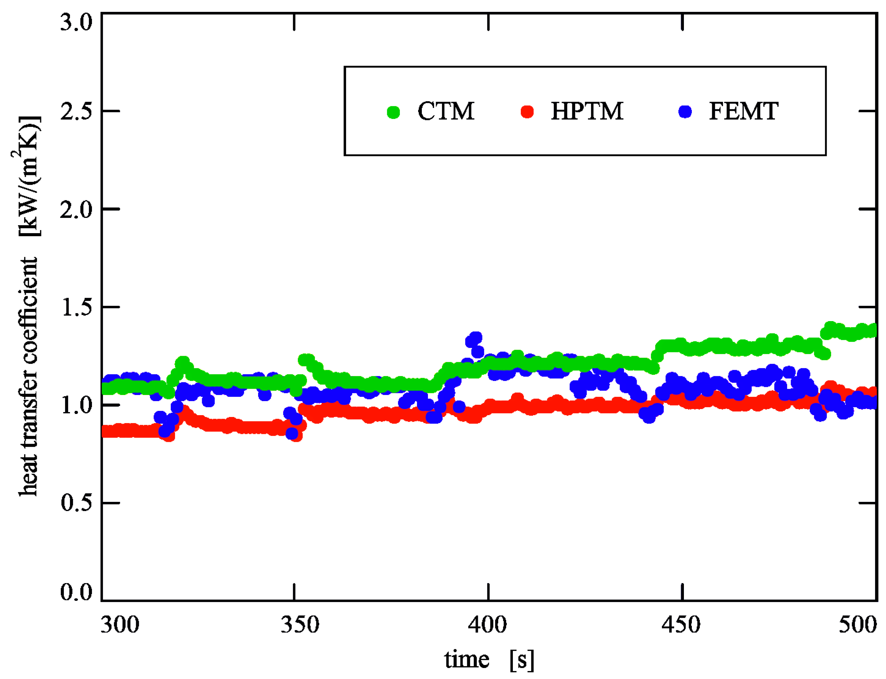
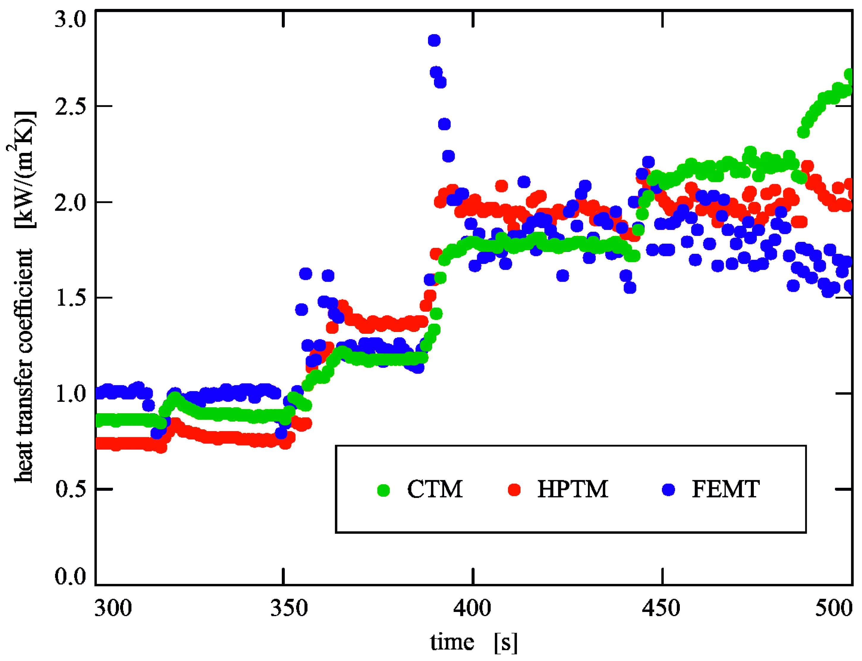
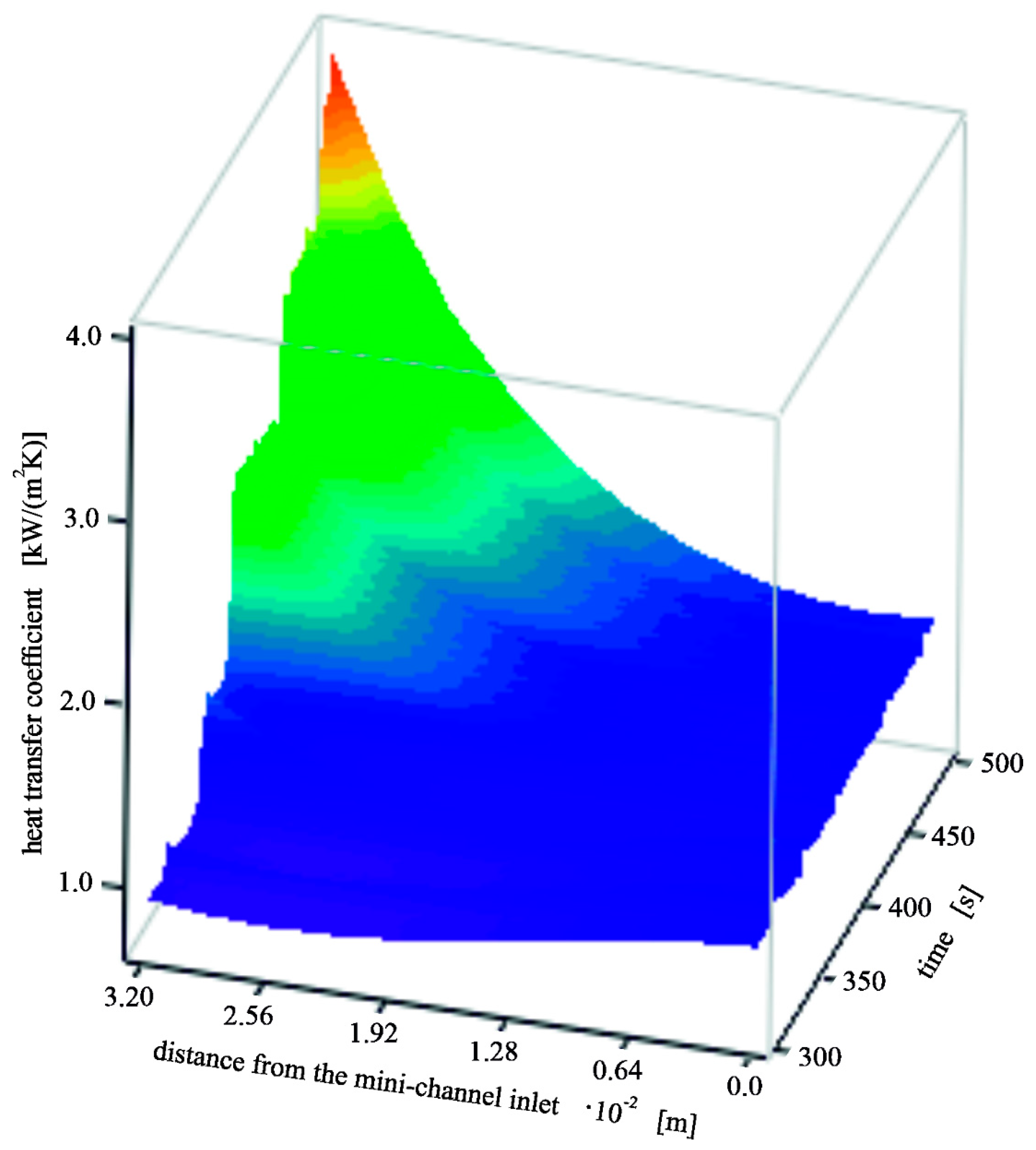
6. Results and Discussion

Numerical calculations were performed for the chosen time interval of the experiment set (from 300 s to 500 s) and the values of the basic experimental parameters are shown in Table 1. In the calculations presented below, the local values of the void fraction (see Figure 5) were approximated either by a step function (for the CTM and the FEMT) or by polynomials (for the HPTM).

The results are presented as the heat transfer coefficient:

• versus distance from the mini-channel inlet and the corresponding two-phase flow patterns—for the four selected time moments (340 s, 380 s, 420 s and 460 s)—Figure 6, Figure 7, Figure 8 and Figure 9;
• versus time—for four selected distances from the mini-channel inlet: x = 0.0114 m, x = 0.0178 m, x = 0.0242 m and x = 0.0306 m—Figure 10, Figure 11, Figure 12 and Figure 13;
• according to the CTM, the HPTM and the FEMT computations versus time and distance from the mini-channel inlet—Figure 14, Figure 15 and Figure 16.

When analyzing the heat transfer coefficient dependence versus distance from the mini-channel inlet, achieved for three time moments: 380 s, 420 s, and 460 s (Figure 7a, Figure 8a and Figure 9a), an increase in coefficient values with the distance is noticed. In these cases, a certain amount of vapor bubbles increasing with time (and supplied heat flux) is observed near the channel outlet (Figure 7b, Figure 8b and Figure 9b), resulting in higher void fraction (up to 8.54%). The local heat transfer coefficients obtained for the first selected moment of time, i.e., 340 s (Figure 6a), are the lowest in comparison with other results. It should be underlined that, although the temperature data indicate the occurrence of subcooled flow boiling, one can hardly see any bubbles (Figure 6b), and the maximum void fraction does not exceed 0.58%. The curves based on the CTM and the HPTM computations show the same trends, whereas the FEMT curves slightly differ from them, indicating a higher sensitivity to the experimental data including void fraction: reaching minimum in the middle of the channel, and the maximum of the coefficient values at the channel inlet and outlet. Furthermore, all plots of heat transfer coefficient appeared to be similar, which confirms the acceptable range of variation of the coefficient.

As can be read from Figure 10, Figure 11, Figure 12 and Figure 13, the heat transfer coefficient increased with time, whereas the highest values were reached at the outlet of the mini-channel (referring to the calculations using the CPM and HPTM). The results for the first selected distance from the mini-channel inlet (0.0114 m) showed a slight variation in the coefficient values (Figure 10). Furthermore, it was observed that the coefficient was the lowest in comparison to the other presented data. Analyzing the data collected at a distance of 0.0306 m from the inlet (Figure 13), it was noticed that the heat conduction coefficient obtained by the FEMT indicated a sudden maximum at the time moment approx. 380 s.

The data illustrated in Figure 14 and Figure 15 concerning the calculation results with the help of the CTM and the HPTM, confirm an increase of the heat transfer coefficient with time and distance from the mini-channel inlet. The highest values of the coefficient were achieved near the channel outlet, for higher values of the heat flux (accompanying increasing distance from the inlet). Local values of the heat transfer coefficient due to the FEMT computations, collected close to the mini-channel inlet, achieve relative high values (see Figure 16) in comparison to the other results.

The heat transfer coefficient calculated by the CTM achieved the highest values compared to the results from the other two methods. Furthermore, the coefficient increases with increasing distance from the mini-channel inlet and with time (Figure 14). Similar values of the heat transfer coefficient were obtained by the HPTM, which follows from inspection (see: Figure 6, Figure 7, Figure 8, Figure 9, Figure 10, Figure 11, Figure 12, Figure 13, Figure 14, Figure 15 and Figure 16). They are additionally confirmed by the maximum relative differences (MRD) which will be discussed in Section 7. While the CTM and the HPTM yield comparable results, the differences between the coefficients from the FEMT computations and the aforementioned methods were higher. It was noticed that the FEMT method reacts faster to dynamic changes in measurements in comparison with the CTM and the HPTM. The growth of vapor phase in the channel (i.e., higher value of void fraction) caused a greater decrease of the heat transfer coefficient calculated by the FEMT than by the other two methods. Moreover, the FEMT looks to be more sensitive to local changes in experimental parameters. A sudden drop in the measured plate temperature, which occurred during the experimental set at the time moment of 400 s, can be observed. It caused an equally sudden jump of the heat transfer coefficient shown in Figure 13. Distinctive features of each calculation method are presented in

Table 3. Distinctive features of the mathematical methods used in calculations.

Distinctive Features	Mathematical Method
	CTM	HPTM	FEMT
Can be used to solve inverse problems	+	+	+
Can be used to solve problems described by a nonlinear differential equation	-	+	-
The solution satisfies exactly the governing differential equation	+	-	+
The solution satisfies exactly the boundary conditions	-	-	+ (*)
The number and the type of boundary conditions (temperature—related, flow-related, discrete or continuous) are not limited	+	+	+
The solution is a differentiable function	-	-	- (**)
Can be applied to problems with complicated geometry	-	-	+
Permits any number of Trefftz functions to be used in the solution	-	-	+ (***)

⁽*⁾ The first-type boundary condition is met only at the boundary nodes of the domain. ⁽**⁾ This property is satisfied for finite elements. ⁽***⁾ The number of Trefftz functions depends on the number of nodes in the element.

.

7. Comparison of the Authors’ Results with Theoretical Correlations

The data from the authors’ own experimental results were used in calculations by the three mathematical methods described above and three theoretical correlations dedicated for small channels. Three correlations were chosen for comparison, namely those proposed by: (i) Lazarek and Black (1982) [57], (ii) Tran et al. (1996) [58], and (iii) Piasecka (2015) [59]. Short characteristics of these correlations are presented in

Table 4. Characteristics of selected theoretical heat transfer correlations concerning small channels.

Author/Authors	Correlation	Characteristics
Lazarek and Black (1982) [57]	${\alpha }_{TP}=30·R{e}_l^{0.857}· B{o}^{0.714}· {\lambda }_l·d_h^{-1}$ (19)	flow boiling heat transfer; the correlation based upon 738 points of R-113, circular mini-channels, hydraulic diameter of channels of 3.15 mm
Tran et al. (1996) [58]	${\alpha }_{TP}=84·{10}^4{\left(B{o}^2·W{e}_l\right)}^{0.3}·{\left(\frac{{\rho }_l}{{\rho }_v}\right)}^{-0.4}$ (20)	flow boiling heat transfer experiments for R-12; hydraulic diameter of channels: 2.46 mm and 2.92 mm
Piasecka (2015) [59]	${\alpha }_{TP}=\Gamma ·{\left(Pe·Bo\right)}^{0.64}·W{e}^{0.46}·{\lambda }_l·d_h^{-1}$ (21)	saturated flow boiling, based on experiments with rectangular mini-channels of 1 mm depth, refrigants R-11, R-123 and FC-72; Γ—surface development parameter

.

The heat transfer coefficients calculated by the presented mathematical methods as well as derived from the chosen theoretical correlations were compared with one another using the authors’ experimental data, namely the data collected at the four time moments: 340 s, 380 s, 420 s, and 460 s. The results are illustrated in Figure 17 as heat transfer coefficient dependence in function of distance from the mini-channel inlet, calculated according to own methods and correlations from the literature. When analysing the results, it was found that the heat transfer coefficient values achieved due to the proposed mathematical methods turned out to be lower in comparison with most of the results computed from theoretical correlations. Moreover, it was noticed that the lowest values of the heat transfer coefficient as the results of FEMT application occurred at the following time moments of the experiment set: 380 s, 420 s, and 460 s, i.e., at higher values of the supplied heat flux.

To thoroughly analyze the results from experiments and calculations according to the proposed mathematical methods and selected theoretical correlations, the maximum relative difference (MRD) between two heat transfer coefficients at the fixed time moment was determined from the following formula:

$$\mathrm{MRD}=max\left\{\frac{\Vert {\alpha }_1-{\alpha }_2\Vert }{\Vert {\alpha }_1\Vert },\frac{\Vert {\alpha }_1-{\alpha }_2\Vert }{\Vert {\alpha }_2\Vert }\right\}·100\%.$$

(22)

The results of calculations according to Equation (22) are listed in

Table 5. Maximum relative differences (MRD) between heat transfer coefficient values calculated from the proposed mathematical methods and selected theoretical correlations at four time moments.

Correlation/Mathematical Method	MRD [%]
t = 340 s
	CTM	HPTM	FEMT
Lazarek and Black (1982)	9	25	9
Tran et al. (1996)	42	68	32
Piasecka (2015)	50	78	39
CTM		20	12
HPTM	20		31
FEMT	12	31
t = 380 s
	CTM	HPTM	FEMT
Lazarek and Black (1982)	7	16	25
Tran et al. (1996)	33	29	43
Piasecka (2015)	44	40	53
CTM		18	12
HPTM	18		19
FEMT	12	19
t = 420 s
	CTM	HPTM	FEMT
Lazarek and Black (1982)	26	36	42
Tran et al. (1996)	20	27	41
Piasecka (2015)	29	35	49
CTM		23	10
HPTM	23		20
FEMT	10	20
t = 460 s
	CTM	HPTM	FEMT
Lazarek and Black (1982)	35	31	42
Tran et al. (1996)	21	33	47
Piasecka (2015)	28	42	56
CTM		26	13
HPTM	26		18
FEMT	13	18

.

According to the data shown in Table 5, the best compliance was found using the correlation by Lazarek and Black, especially for the initial time moments of the experimental set. For the remaining correlations, MRDs take higher values and reach even 78%. The highest MRD for the results obtained by theoretical correlations was for the HPTM at t = 340 s. However, when the heat flux increases, the FEMT gives the results whose MRD achieves higher values than for other methods.

The MRDs between the results obtained by the CTM and the HPTM and the results obtained by the CTM and the FEMT take higher values. Except for the results obtained for t = 340 s, it was noticed that the MRD increases with heat flux (and the void fraction) for the CTM and the HPTM methods. However, the MRD does not exceed 31%, regardless of the method applied.

8. Conclusions

This work focuses on the mathematical modeling of time-dependent heat transfer process during flow boiling in a mini-channel heat sink. The data from the experimental set conducted on the set-up with the test section comprising five mini-channels of 1 mm depth. During the experiment, the test section was inclined (75°) to the horizontal plane. An infrared camera recorded the temperature field on the outer heated surface of the mini-channel wall while a high-speed camera was monitoring two-phase flow patterns, simultaneously. Based on the saved images during the experiment, after their analyses using own software, void fraction in 10 areas along the flow was determined and used in further calculations.

Having proposed a mathematical model of the posed problem, the aim was to identify the heat transfer coefficient on the heated wall-fluid contact surface. In terms of mathematical computations, the coefficient which appears in the Robin boundary condition should be somehow evaluated. Three methods based on Trefftz functions, namely the FEM with Trefftz-type basis functions (FEMT), the Classical Trefftz Method (CTM), and the Hybrid Picard-Trefftz Method (HPTM), were used in the paper for numerical calculations. The methods are effective in solving the inverse heat transfer problems. The proposed methods allowed calculating two-dimensional time-dependent temperature distributions in two contacting areas: the heater plate and the flowing fluid. In particular, the HPTM method is useful in solving time-dependent nonlinear problems. The CTM and the HPTM methods do not require the use of an advanced mathematical apparatus. The FEMT can be employed to solve problems in the domains of very complicated shapes. In this method, the set of nodes in the domain can be adjusted to the temperature measurements for exactly fulfilling the boundary conditions in nodes. Compared with the other methods presented in this article, a smaller number of the Trefftz functions can be used to approximate the solution of the given problem. The numerical results obtained from the proposed mathematical model and three calculation methods were validated by comparing them to the results gained using theoretical correlations. The comparison between the heat transfer coefficients, calculated by the tested mathematical methods and achieved from three correlations selected from the literature, all based on the data from the authors’ experiments, gave satisfactory results. The best compliance was found by using the correlation by Lazarek and Black. The analysis proved that the values of temperature and heat transfer coefficient were similar.

In the near future, the research will focus on: (i) adaptation of the mathematical model to heat transfer problems with higher void fraction and including different mini-channel inclinations to the horizontal plane, (ii) improvement of the proposed calculation methods, and (iii) comparing the results from the Trefftz functions to those obtained with the help of commercial software, like ANSYS CFX/Fluent and STAR-CCM+. It is expected that the results of experimental studies will widen the knowledge of heat transfer during flow boiling in mini- and micro-channel heat sinks within a wide range of thermal and flow parameters, for various geometries and spatial orientation of the channels. Such a wide experimental research combined with the application of numerical methods will certainly provide a big amount of data.

The confrontation of the mathematical model and advanced computational methods with the experiment will allow for a detailed understanding of heat transfer processes occurring during flow boiling in mini-channels. It is worth to underline that the flow boiling heat-transfer process during fluid flow in mini-channels may find practical application in modern miniaturization of devices used in electronics, transportation, nuclear technology, medicine, and other energy brands. Compact heat exchangers with minigaps are strongly needed as the elements of computer units, which require intensive cooling. The calculation results could be useful for designing cooling systems in mini-scale—as mini-channel heat exchangers.

References

1. Piasecka, M.; Maciejewska, B.; Łabędzki, P. Heat Transfer Coefficient Determination during FC-72 Flow in a Minichannel Heat Sink Using the Trefftz Functions and ADINA Software. Energies 2020, 13, 6647. [Google Scholar] [CrossRef]
2. Zaborowska, I.; Grzybowski, H.; Rafalko, G.; Mosdorf, R. Boiling dynamics in parallel minichannel system with different inlet solutions. Int. J. Heat Mass Transf. 2021, 165, 120655. [Google Scholar] [CrossRef]
3. Kuczynski, W.; Bohdal, T.; Meyer, J.P.; Denis, A. A regressive model for dynamic instabilities during the condensation of R404A and R507 refrigerants. Int. J. Heat Mass Transf. 2019, 141, 1025–1035. [Google Scholar] [CrossRef]
4. Klugmann, M.; Dabrowski, P.; Mikielewicz, D. Flow distribution and heat transfer in minigap and minichannel heat exchangers during flow boiling. Appl. Therm. Eng. 2020, 181, 116034. [Google Scholar] [CrossRef]
5. Moreira, T.A.; Furlan, G.; de Sena e Oliveira, G.H.; Ribatski, G. Flow boiling and convective condensation of hydrocarbons: A state-of-the-art literature review. Appl. Therm. Eng. 2021, 182, 116129. [Google Scholar] [CrossRef]
6. Kruzel, M.; Bohdal, T.; Sikora, M. Heat transfer and pressure drop during refrigerants condensation in compact heat exchangers. Int. J. Heat Mass Transf. 2020, 161, 120283. [Google Scholar] [CrossRef]
7. Manetti, L.L.; Ribatski, G.; de Souza, R.R.; Cardoso, E.M. Pool boiling heat transfer of HFE-7100 on metal foams. Exp. Therm. Fluid Sci. 2020, 113, 110025. [Google Scholar] [CrossRef]
8. Pastuszko, R.; Kaniowski, R.; Wójcik, T.M. Comparison of pool boiling performance for plain micro-fins and micro-fins with a porous layer. Appl. Therm. Eng. 2020, 166, 114658. [Google Scholar] [CrossRef]
9. Orman, L.J.; Radek, N.; Pietraszek, J.; Szczepaniak, M. Analysis of Enhanced Pool Boiling Heat Transfer on Laser-Textured Surfaces. Energies 2020, 13, 2700. [Google Scholar] [CrossRef]
10. Błasiak, S. Influence of Thermoelastic Phenomena on the Energy Conservation in Non-Contacting Face Seals. Energies 2020, 13, 5283. [Google Scholar] [CrossRef]
11. Joachimiak, D.; Frąckowiak, A. Experimental and Numerical Analysis of the Gas Flow in the Axisymmetric Radial Clearance. Energies 2020, 13, 5794. [Google Scholar] [CrossRef]
12. Piasecka, M.; Strąk, K.; Grabas, B. Vibration-Assisted Laser Surface Texturing and Electromachining for the Intensification of Boiling Heat Transfer in a Minichannel. Arch. Metall. Mater. 2017, 62, 1983–1990. [Google Scholar] [CrossRef]
13. Piasecka, M.; Strąk, K. Influence of the Surface Enhancement on the Flow Boiling Heat Transfer in a Minichannel. Heat Transf. Eng. 2019, 40, 1162–1175. [Google Scholar] [CrossRef]
14. Maciejewska, B.; Piasecka, M. Time-dependent study of boiling heat transfer coefficient in a vertical minichannel. Int. J. Numer. Methods Heat Fluid Flow 2019, 30, 2953–2969. [Google Scholar] [CrossRef]
15. Maciejewska, B.; Piasecka, M.; Piasecki, A. The Study of the Onset of Flow Boiling in Minichannels—Time-Dependent Heat Transfer Results. Heat Transf. Eng. 2021, 43, 1–15. [Google Scholar] [CrossRef]
16. Hożejowska, S.; Piasecka, M. Numerical Solution of Axisymmetric Inverse Heat Conduction Problem by the Trefftz Method. Energies 2020, 13, 705. [Google Scholar] [CrossRef] [Green Version]
17. Maciejewska, B.; Błasiak, S.; Piasecka, M. Determination of the temperature distribution in a minichannel using ANSYS CFX and a procedure based on the Trefftz functions. EPJ Web Conf. 2017, 143, 02071. [Google Scholar] [CrossRef] [Green Version]
18. Jaszczur, M.; Mlynarczykowska, A.; Demurtas, L. Effect of Impeller Design on Power Characteristics and Newtonian Fluids Mixing Efficiency in a Mechanically Agitated Vessel at Low Reynolds Numbers. Energies 2020, 13, 640. [Google Scholar] [CrossRef] [Green Version]
19. Guo, Z.; Fletcher, D.F.; Haynes, B.S. A review of computational modelling of flow boiling in microchannels. J. Comput. Multiph. Flows 2014, 6, 79–110. [Google Scholar] [CrossRef] [Green Version]
20. Hadamard, J. Sur les Problèmes aux Dérivées Partielles et Leur Signification Physique. Princet. Univ. Bull. 1902, 13, 49–52. [Google Scholar]
21. Kita, E.; Kamiya, N. Trefftz method: An overview. Adv. Eng. Softw. 1995, 24, 3–12. [Google Scholar] [CrossRef]
22. Li, Z.-C.; Lu, T.-T.; Huang, H.-T.; Cheng Alexander, H.-D. Trefftz, collocation, and other boundary methods—A comparison. Numer. Methods Partial Differ. Equ. 2006, 23, 1–52. [Google Scholar] [CrossRef]
23. Grysa, K.; Maciag, A.; Pawinska, A. Solving nonlinear direct and inverse problems of stationary heat transfer by using Trefftz functions. Int. J. Heat Mass Transf. 2012, 55, 7336–7340. [Google Scholar] [CrossRef]
24. Hożejowska, S.; Maciejewska, B.; Poniewski, M.E. Numerical Analysis of Boiling Two-Phase Flow in Mini- and Microchannels. In Encyclopedia of Two-Phase Heat Transfer and Flow I. Fundamentals and Method. Vol. 4 Specjal Topics in Pool and Flow Boiling; Thome, J.R., Ed.; World Scientific Publishing Co., Ltd.: New York, NY, USA; London, UK; Singapore, 2016; pp. 131–160. [Google Scholar]
25. Trefftz, E. Ein Gegenstück zum Ritzschen Verfahren. In Proceedings of the International Kongress für Technische Mechanik, Zürich, Switzerland, 12–17 September 1926; pp. 131–137. [Google Scholar]
26. Herrera, I. Trefftz method: A general theory. Numer. Methods Partial Differ. Equ. 2000, 16, 561–580. [Google Scholar] [CrossRef]
27. Grysa, K.; Maciejewska, B. Trefftz functions for non-stationary problems. J. Theor. Appl. Mech. 2013, 51, 251–264. [Google Scholar]
28. Alves, C.; Karageorghis, A.; Leitão, V.; Valtchev, S. (Eds.) Advances in Trefftz Methods and Their Applications; Springer: Cham, Germany, 2020. [Google Scholar]
29. Cialkowski, M.; Frackowiak, A. Solution of the stationary 2D inverse heat conduction problem by Treffetz method. J. Therm. Sci. 2002, 11, 148–162. [Google Scholar] [CrossRef]
30. Movahedian, B.; Boroomand, B.; Soghrati, S. A Trefftz method in space and time using exponential basis functions: Application to direct and inverse heat conduction problems. Eng. Anal. Bound. Elem. 2013, 37, 868–883. [Google Scholar] [CrossRef]
31. Moldovan, I.D.; Coutinho, A.; Cismasiu, I. Hybrid-Trefftz finite elements for non-homogeneous parabolic problems using a novel dual reciprocity variant. Eng. Anal. Bound. Elem. 2019, 106, 228–242. [Google Scholar] [CrossRef]
32. Grysa, K.; Maciag, A. Temperature dependent thermal conductivity determination and source identification for nonlinear heat conduction by means of the Trefftz and homotopy perturbation methods. Int. J. Heat Mass Transf. 2016, 100, 627–633. [Google Scholar] [CrossRef]
33. Blasiak, S.; Pawinska, A. Direct and inverse heat transfer in non-contacting face seals. Int. J. Heat Mass Transf. 2015, 90, 710–718. [Google Scholar] [CrossRef]
34. Cialkowski, M. New type of basic functions of FEM in application to solution of inverse heat conduction problem. J. Therm. Sci. 2002, 11, 163–171. [Google Scholar] [CrossRef]
35. Grysa, K.; Hożejowska, S.; Maciejewska, B. Adjustment calculus and Trefftz functions applied to local heat transfer coefficient determination in a minichannel. J. Theor. Appl. Mech. 2012, 50, 1087–1096. [Google Scholar]
36. Qin, Q.-H. Trefftz Finite Element Method and Its Applications. Appl. Mech. Rev. 2005, 58, 316–337. [Google Scholar] [CrossRef]
37. Qin, Q.-H. The Trefftz Finite and Boundary Element Method; WIT Press: Southampton, UK, 2000. [Google Scholar]
38. Hożejowska, S. Homotopy perturbation method combined with Trefftz method in numerical identification of liquid temperature in flow boiling. J. Theor. Appl. Mech. 2015, 53, 969–980. [Google Scholar] [CrossRef] [Green Version]
39. Uscilowska, A. Application of the Trefftz method to nonlinear potential problems. Computer Assisted Mechanics and Engineering Sciences. In Proceedings of the Lsame.08: Leuven Symposium on Applied Mechanics in Engineering, PTS 1 and 2, Louvain, Belgium, 31 March–2 April 2008; pp. 417–431. [Google Scholar]
40. Grabowski, M.; Poniewski, M.E.; Hożejowska, S.; Pawińska, A. Numerical simulation of the temperature fields in a single-phase flow in an asymmetrically heated mininchannel. J. Eng. Phys. Thermophys. 2020, 93, 355–363. [Google Scholar] [CrossRef]
41. Węgrzyn, T.; Szczucka-Lasota, B.; Uscilowska, A.; Stanik, Z.; Piwnik, J. Validation of parameters selection of welding with micro-jet cooling by using method of fundamental solutions. Eng. Anal. Bound. Elem. 2019, 98, 17–26. [Google Scholar] [CrossRef]
42. Yang, A.-M.; Zhang, C.; Jafari, H.; Cattani, C.; Jiao, Y. Picard Successive Approximation Method for Solving Differential Equations Arising in Fractal Heat Transfer with Local Fractional Derivative. Abstr. Appl. Anal. 2014, 1–5. [Google Scholar] [CrossRef]
43. Ince, E.L. Ordinary Differential Equations; Dover Publications, Inc.: New York, NY, USA, 1956. [Google Scholar]
44. Picard, E. Sur l’application des méthodes d’approximations successives à l’étude de certaines équations différentielles ordinaires. J. Math. Pures Appl. 1893, 9, 217–272. [Google Scholar]
45. Bellman, R.E.; Kalaba, R.E. Quasi Linearization and Nonlinear Boundary-Value Problems; American Elsevier Publishing Company: New York, NY, USA, 1965. [Google Scholar]
46. Clenshaw, C.W.; Norton, H.J. The solution of nonlinear ordinary differential equations in Chebyshev series. Comput. J. 1963, 6, 88–92. [Google Scholar] [CrossRef] [Green Version]
47. Hożejowski, L.; Hożejowska, S. Trefftz method in an inverse problem of two-phase flow boiling in a minichannel. Eng. Anal. Bound. Elem. 2019, 98, 27–34. [Google Scholar] [CrossRef]
48. Michalski, D.; Strąk, K.; Piasecka, M. Estimating uncertainty of temperature measurements for studies of flow boiling heat transfer in minichannels. EPJ Web Conf. 2019, 213, 1–7. [Google Scholar] [CrossRef]
49. Grabowski, M.; Hozejowska, S.; Maciejewska, B.; Placzkowski, K.; Poniewski, M.E. Application of the 2-D Trefftz Method for Identification of Flow Boiling Heat Transfer Coefficient in a Rectangular MiniChannel. Energies 2020, 13, 3973. [Google Scholar] [CrossRef]
50. Maciejewska, B.; Piasecka, M. Trefftz function-based thermal solution of inverse problem in unsteady-state flow boiling heat transfer in a minichannel. Int. J. Heat Mass Transf. 2017, 107, 925–933. [Google Scholar] [CrossRef]
51. Bohdal, T. Modeling the process of bubble boiling on flows. Arch. Thermodyn. 2000, 21, 34–75. [Google Scholar]
52. Hożejowska, S.; Kaniowski, R.; Poniewski, M.E. Experimental investigations and numerical modeling of 2D temperature fields in flow boiling in minichannels. Exp. Therm. Fluid Sci. 2016, 78, 18–29. [Google Scholar] [CrossRef]
53. Tolubinski, V.I.; Kostanchuk, D.M. Vapour bubbles growth rate and heat transfer intensity at subcooled water boiling. In Proceedings of the 4th Int. Heat Transfer Conference, Paris-Versailles, France, 31 August–5 September 1970; pp. 1–11. [Google Scholar]
54. Koncar, B.; Matkovic, M.; Prosek, A. NEPTUNE_CFD Analysis of Flow Field in Rectangular Boiling Channel. J. Comput. Multiph. Flows 2012, 4, 399–410. [Google Scholar] [CrossRef] [Green Version]
55. Cheung, Y.K.; Jin, W.G.; Zienkiewicz, O.C. Direct solution procedure for solution of harmonic problems using complete, non-singular, Trefftz functions. Commun. Appl. Numer. Methods 1989, 5, 159–169. [Google Scholar] [CrossRef]
56. Grabowski, M.; Hożejowska, S.; Pawińska, A.; Poniewski, M.; Wernik, J. Heat Transfer Coefficient Identification in Mini-Channel Flow Boiling with the Hybrid Picard–Trefftz Method. Energies 2018, 11, 2057. [Google Scholar] [CrossRef] [Green Version]
57. Lazarek, G.M.; Black, S.H. Evaporative heat transfer, pressure drop and critical heat flux in a small vertical tube. Int. J. Heat Mass Transf. 1982, 25, 945–960. [Google Scholar] [CrossRef]
58. Tran, T.N.; Wambsganss, M.W.; France, D.M. Small circular- and rectangular-channel boiling with two refrigerants. Int. J. Multiph. Flow 1996, 22, 485–498. [Google Scholar] [CrossRef]
59. Piasecka, M. Correlations for flow boiling heat transfer in minichannels with various orientations. Int. J. Heat Mass Transf. 2015, 81, 114–121. [Google Scholar] [CrossRef]
Figure 1. The experimental apparatus: 1—test section, 2—gear pump, 3—compensating tank, 4—heat exchanger, 5—filter, 6—Coriolis mass flow meter, 7—deaerator, 8—PC computer, 9—infrared camera, 10—high-speed digital camera.
Energies 14 01832 g001
Figure 2. The test section: (a) cross-section, (b) front view, 1—front cover, 2—mini-channel manifold, 3—glass plate, 4—mini-channel, 5—heated plate, 6—channel body.
Energies 14 01832 g002
Figure 3. Temperature of the heated plate from infrared measurement versus time and distance from the mini-channel inlet; experimental parameters are listed in Table 1.
Energies 14 01832 g003
Figure 4. A scheme showing the distribution of areas corresponding to two-phase flow patterns, assumed for void fraction calculation.
Energies 14 01832 g004
Figure 5. Void fraction versus time and distance from the mini-channel inlet; experimental parameters are listed in Table 1.
Energies 14 01832 g005
Figure 6. (a) Heat transfer coefficient versus distance from the mini-channel inlet, (b) two-phase flow pattern, t = 340 s; other experimental parameters are listed in Table 1.
Energies 14 01832 g006
Figure 7. (a) Heat transfer coefficient versus distance from the mini-channel inlet, (b) two-phase flow pattern, t = 380 s, other experimental parameters listed in Table 1.
Energies 14 01832 g007
Figure 8. (a) Heat transfer coefficient versus distance from the mini-channel inlet, (b) two-phase flow pattern, t = 420 s; other experimental parameters are listed in Table 1.
Energies 14 01832 g008
Figure 9. (a) Heat transfer coefficient versus distance from the mini-channel inlet, (b) two-phase flow pattern, t = 460 s; other experimental parameters are listed in Table 1.
Energies 14 01832 g009
Figure 10. Heat transfer coefficient versus time, the distance from the mini-channel inlet x = 0.0114 m; other experimental parameters are listed in Table 1.
Energies 14 01832 g010
Figure 11. Heat transfer coefficient versus time, the distance from the mini-channel inlet x = 0.0178 m; other experimental parameters are listed in Table 1.
Energies 14 01832 g011
Figure 12. Heat transfer coefficient versus time, the distance from the mini-channel inlet x = 0.0242 m; other experimental parameters are listed in Table 1.
Energies 14 01832 g012
Figure 13. Heat transfer coefficient versus time, the distance from the mini-channel inlet x = 0.0306 m; other experimental parameters are listed in Table 1.
Energies 14 01832 g013
Figure 14. Heat transfer coefficient according to the CTM computation versus time and distance from the mini-channel inlet; experimental parameters are listed in Table 1.
Energies 14 01832 g014
Figure 15. Heat transfer coefficient according to the HPTM computation versus time and distance from the mini-channel inlet; experimental parameters are listed in Table 1.
Energies 14 01832 g015
Figure 16. Heat transfer coefficient according to the FEMT computation versus time and distance from the mini-channel inlet; experimental parameters are listed in Table 1.
Energies 14 01832 g016
Figure 17. Heat transfer coefficient versus the distance from the mini-channel inlet, calculated according to proposed mathematical methods and theoretical correlations from the literature, based on the data collected at the following time moments of the experimental set: (a) 340 s, (b) 380 s, (c) 420 s, and (d) 460 s; experimental parameters are listed in Table 1.
Energies 14 01832 g017