Analysis of Multi-Stream Fuel Injector Flow Using Zonal Proper Orthogonal Decomposition

Abstract

The 3-component velocity distribution of two lean-burn gas turbine fuel injectors are measured at a planar location near and parallel to the injector outlet. The two injectors are nominally the same design, but one features blocked central passages to study the effects of the presence of multi-streams and reveal the single stream characteristics embedded within the multi-stream configuration. Stereoscopic particle image velocimetry is used in an isothermal, non-reacting water analogue flow facility at an engine relevant Reynolds number. The velocity data is analysed using proper orthogonal decomposition (POD) and the work introduces the concept of Zonal POD. This is the splitting of the velocity field into zones prior to the calculation of POD modes to better identify prominent structures and features associated with each zone. Because modes are sorted by the area averaged energy contribution, zoning of a velocity field of interest may change the individual modes and will almost certainly change their order for anything other than trivial flow fields. Analysis of ensemble average and velocity fluctuation profiles reveals a radial shift outboard of the mains flow with the presence of the pilot as well as a general increase in RMS across the intermediate region between the pilot and mains flows. Analysis of POD temporal coefficients in the frequency domain reveals a low-frequency peak is evident in the mains flow region, but which may be affected by the presence of pilot flow. Furthermore, application of the ZPOD technique results in a closer representation of the velocity data for a given number of modes. This shows the behaviour of the unsteady pilot flow and reveals that a significant proportion of the fluctuating energy, RMS, is caused by this characteristic.

1. Introduction

As with other segments of the transport industries, civil aviation is under pressure to reduce the environmental impact through improved fuel efficiency and a reduction in emissions of CO₂, NO_X, CO, unburnt hydrocarbons and particulate matter. There is stringent aviation legislation in place that is constantly evolving to limit the environmental impact of aircraft and specifically aero gas turbine engines.

Lean burn technology is one of the prevailing approaches to achieving this goal, specifically with regards to reduction of NO_X emission. The injectors used in lean-burn combustion systems must admit a significantly greater proportion of the compressor efflux in comparison to their rich-burn counterparts. To accommodate this increased airflow, which may be up to 70% of the compressor efflux, the injectors are physically larger to keep pressure drops to an acceptable level. This considerable change in geometry of what is in effect an aerodynamic device requires new characterisation of injector outflow. Airflow structures in and around the injector are key to many combustion and fuel preparation processes such as fuel film break-up, atomization and distribution of air–fuel ratio. These factors, particularly the local air–fuel ratio, are important in the understanding and control of the formation of CO, CO₂ and NO_X as outlined by Lefebvre [1]. Furthermore, injector spatial and temporal instabilities can alter the flow field and lead to combustion instability [2], which brings with it potential issues with efficiency and noise.

Modern fuel injectors, in both rich and lean burn systems, generally use swirl to provide a stable flame environment. As discussed by Beèr and Chigier [3], the high radial pressure gradients associated with swirling flows lead to vortex breakdown and high shear, promoting fuel break-up and mixing. Injectors must achieve a sufficiently large swirl number, beyond the critical value of 0.5–0.6, to cause a central toroidal recirculation zone to form which has the effect of anchoring and stabilizing the flame [3]. In addition, Syred and Beèr suggest the presence of this structure improves combustion efficiency and reduces flame length [4].

The fuel injectors have a complex downstream flow with multiple swirling airstreams interacting with each other. Lin et al. [5] used PIV to measure velocity at a nearfield plane and found the shedding of large coherent structures. The associated temporal fluctuations were found to have a major impact on combustion stability in work by Schildmacher and Koch [6] in airblast spray.

Due to the significant impact on engine performance, there is the need to further understand the characteristics and unsteady nature of structures and frequencies in lean-burn injectors. In this work we investigate the velocity distribution and prominent flow features of a multi-stream, lean-burn injector. The objectives are to identify features from within either the mains or pilot regions and the effects of any interaction between them on spatial or temporal characteristics. This will be carried out over a single parallel (R-θ) plane at the injector outlet for an engine relevant Reynolds number.

2. Experimental Methodology

Sets of experimentally acquired velocity data via stereo-PIV for two similar injector geometries are analysed. The two sets consist of a common multi-stream lean-burn type gas turbine fuel injector in which one model has several flow streams blocked to provide distinct differences in their flow field characteristic. The remainder of this section describes the experimental flow facility, test hardware and data processing parameters.

2.1. Water Flow Test Facility and Data Acquisition

All presented fluid velocity measurements were carried out in the Loughborough University vertical flow water test facility, depicted in Figure 1. The test facility is designed to allow high optical accessibility in a wide range of measurement volume regions around injectors and swirling geometries for common optical diagnostic techniques such as stereo-PIV and tomographic-PIV.

The test facility provides a water analogue to typically aerodynamic devices by Reynolds number matching engine representative airflow rates and has several features to improve the test quality. Firstly, by using a closed loop system, as depicted in Figure 1, flow seeding may be carefully dosed and then will remain constant throughout all testing, with fluid remaining useable for a significant number of tests before refreshing is required. Secondly, the use of a header-tank arrangement removes any pulse characteristics that may otherwise be present in a pump driven flow; this is used in series with throttle valves downstream of the injector to control pressure-drop, and therefore flowrate through the device. Finally, a specifically designed water jacket with angled viewing windows minimizes optical distortion due to camera viewing angles. Further details, including a photograph of the test rig in a similar optical arrangement can be seen in Spencer et al. [7].

Mass flow rate, and therefore calculated Reynolds number, is monitored and set using the mass flow meter, located downstream of the control valves. A National Instruments Labview program is used to display real-time calculation of Reynolds number as well as logging this value, mass flow rate and sump temperature during testing. The latter is found to stabilize after a brief warm-up period but nevertheless is monitored throughout testing to maintain constant mass flow and volume flow rates, and therefore calculated Reynolds number.

The use of water as a flow medium offers numerous advantages over testing with gas-phase flow. For example, from a practical perspective, the seeding of the flow is much simpler in water as particles may be added to the sump in known quantities and allowed to circulate in order to mix homogeneously. The seeding used in all presented experiments was PSP Polyamide seeding particles with mean diameter of 20 µm (Dantec Dynamics) which have a density of 1.03 g/cm³, i.e., very close to the flow medium (1.0 g/cm³). This minimizes particle slippage, ensuring minimal error in the measurement of representative particle (and therefore fluid) velocity. The low slippage also prevents regions of sparse seeding which can occur for example in the centre of vortices. While this may not be eliminated, this process happens over a longer time than the typical experiment would allow and therefore there was no evidence of this in any of the presented work. This element and other error considerations are discussed in detail in Spencer et al. [7].

Stereoscopic PIV is used to measure 3-component velocity distributions at 12 Hz on a downstream plane, perpendicular to injector axial flow direction as shown in Figure 1. A Litron Nano L 135-15 dual-cavity Nd:YAG laser is used to provide illumination. The pulsed 532 nm beam with 108 mJ energy is guided via LaVision guiding arm and directed through sheet optics (LaVision) with final focal length, f = −20 mm to form a 1 mm thick sheet sufficient to cover the measurement plane located 12 mm downstream of the injector outlet.

Two LaVision Imager ProX4 double-frame cameras with 4 MPix resolution (2048 × 2048, 7.4 µm) were mounted viewing perpendicularly to the angled windows as indicated in Figure 1, approximately 45° relative to the injector axis. The cameras were each fitted with a Nikkor macro lens with focal length, f = 60 mm via a Scheimpflug mount, adjusted to the appropriate angle to maintain focus over the measurement plane. A 532 nm CWL, 10 nm FWHM bandpass filter (Andover Optics) was fitted to each of the cameras to suppress background light.

All timing and synchronisation was via the LaVision Programmable Timing Unit (PTU9) at a rate of 12 Hz and interframe time of 80 µs. The process was manually triggered to capture a dataset of 1200 image pairs, covering a duration of 100 s. Flow was allowed through the injector for at least several seconds before triggering of the acquisition—this served to ensure that any settled seeding particles in the geometry were carried away, and to allow a steady flow-rate measurement.

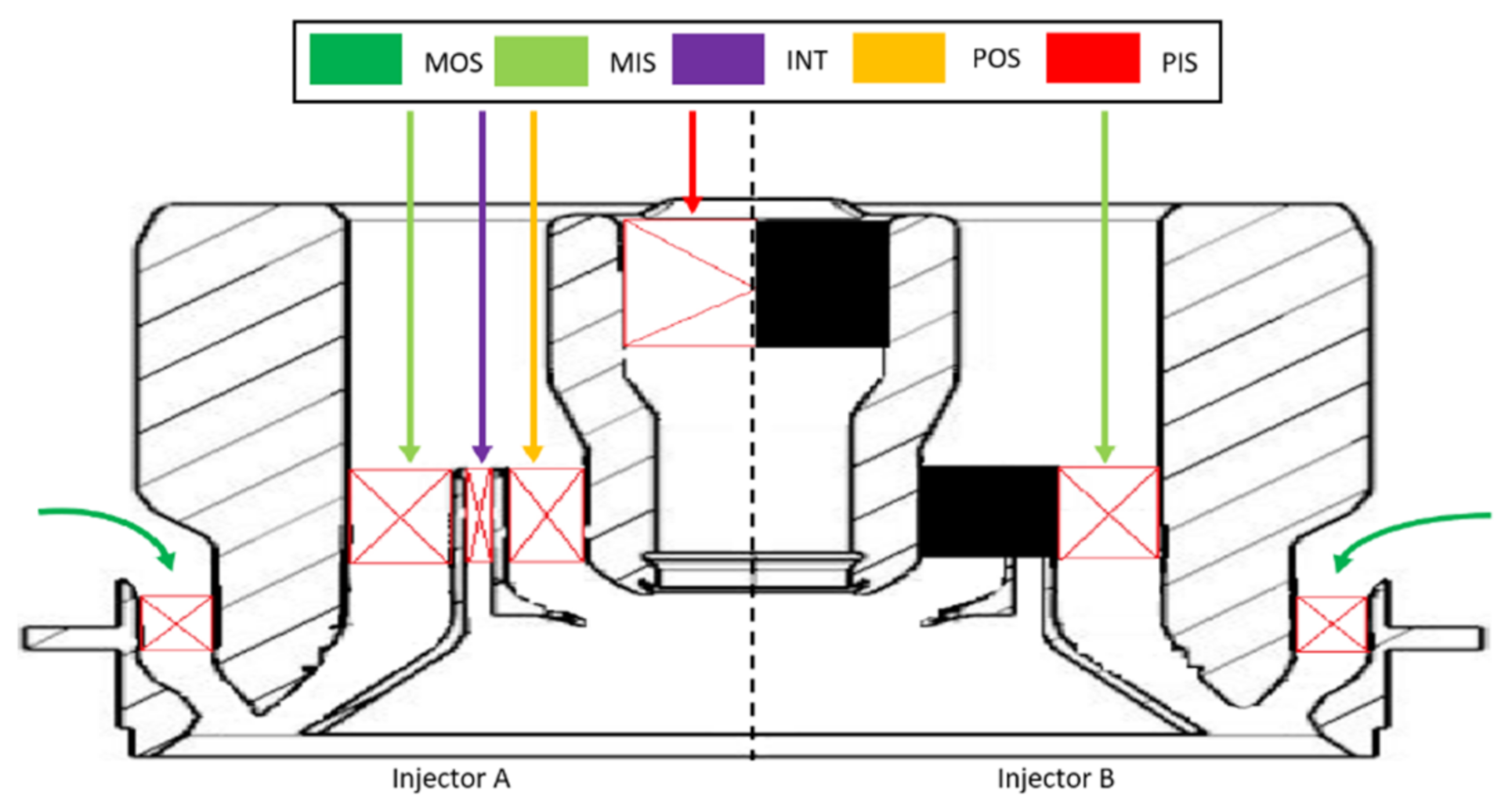
2.2. Test Geometry and Conditions Details

The models used for the presented work are based on a typical lean-burn type gas turbine fuel injector. Salient characteristics of these injectors include a flow of a greater proportion of the compressor efflux—~70% compared to ~30% in their rich-burn counterparts—leading to a comparably larger physical dimension. The type used in this work was a multi-passage swirling type with counter-rotating airstreams, shown in Figure 2. The LHS of Figure 2. represents the baseline geometry, with indicative locations of swirl blades marked. Figure 2 also serves to define the terminology used throughout this work, in line with other published work [8]. These are mains outer (MOS), mains inner (MIS), intermediate (INT), pilot outer (POS) and pilot inner (PIS).

Both injectors were manufactured using rapid prototype methods and are the same design in aspects, other than the indicated blocked PIS, POS and INT passages (Figure 2). The two injectors therefore have differing geometric and effective flow areas. The former is considered here in order to scale the rig flow-rate settings for Injector B tests to ensure comparable velocities, and therefore Reynolds number, are observed through the common mains passages (MIS and MOS). However, by altering the passage flow distribution in this manner, the contribution to dominating structures in the downstream flow may be investigated.

All data reported in this work is with reference to the bulk average velocity, which is calculated according to:

$$V_{ref}=\frac{4\dot{m}}{\pi \rho D_I^2}=\frac{\dot{m}}{\rho A_g}$$

(1)

where $\dot{m}$ is the mass flow rate, $D_I$ is the injector diameter, and $A_g$ is the geometric area. Spatial coordinates are non-dimensionalised by R_ref, which is taken as half of the injector diameter. For calculation of Reynolds number, the injector diameter and average velocity is considered. Due to the scaling previously discussed, this is equivalent for each injector set, $R{e}_D\cong \mathrm{91,000}$.

2.3. PIV and Further Vector Processing

All acquisition and image/vector processing (prior to application of ZPOD and POD analysis) is carried out using the LaVision DaVis v8.4 commercial software package. Stereo calibration was achieved using a stepped plate submerged in the filled rig, but without any moving flow to ensure optical paths have applicable refractive index. A 3rd order polynomial model was fitted to the image data transformation with an RMS fit of 0.003 and 0.006 pixel for camera 1 and 2 respectively.

Acquired image sets had two pre-processing operations applied. Minimum values over a symmetrical five-frame window were subtracted to remove background artifacts such as constant reflections. Geometric masking was applied to the region of interest for vector calculation.

Vector calculation was performed via the widely used stereo cross-correlation technique with multiple passes of decreasing window size. Initially, two passes with windows of size 96 × 96 and 50% overlap were carried out, followed by three further passes with 32 × 32 windows and 75% overlap. Multi-pass processing steps included vector acceptance based on rejecting (peak) Q ratio < 1.3 and the universal outlier detection algorithm [9]. For the final pass of vector processing, the criterion for Q ratio was reduced to 1.1. Using the described process, each vector field consisted of 12,300 vectors with typical vector acceptance greater than 99%.

Figures throughout the following sections are presented in both cartesian and, where appropriate, polar coordinate systems to aid visualization of features discussed. The transformation to polar coordinates and components is carried out only prior to display, and all calculations, including ZPOD and POD, were carried out on the Cartesian dataset. This is an important distinction to make, as interpolation between grids is required and this can introduce artifacts in modal energy distribution due to the resolution difference, particularly as $r\to 0$. However, this is not relevant when considering the figures for display only and is therefore not discussed any further in this paper but offered as a point for consideration for similar work.

2.4. Proper Orthogonal Decomposition

Modal decomposition and low-order modelling techniques allow for the identification and characterization of flow features in fluid mechanics measurements. Since its introduction by Lumley [10], proper orthogonal decomposition (POD) has become commonplace in the analysis of velocity data. POD is one of several modal analysis techniques and is the focus of this section. For a comprehensive review of modal analysis in fluid mechanics, the reader is referred to work by Taira et al. [11]. In this context, POD decomposes the fluctuating velocity field into a set of N basis functions or spatial modes, φ(x), and a related temporal coefficient, a(t), according to

$$\mathit{u}\left(\mathit{x},t_i\right)=\overline{U}\left(\mathit{x}\right)+{\displaystyle \sum }_{k=1}^N{a}_k\left(t_i\right){\mathit{\phi }}_k\left(\mathit{x}\right) i=1,\dots ,N$$

(2)

where u and $\overline{U}$ represent the velocity field at time t and the time-averaged velocity field respectively. The spatial modes are determined by solving the eigenvalue problem with each value representing the energy content of the respective mode. It is usual to order the modes by energy content such that the early modes (k = 1, 2, 3 …) contain the most energetic contributions of velocity fluctuation. In other words, each subsequent mode (k = n + 1) contains less energy than the previous one (k = n) as averaged over the domain, x. In datasets where the spatial resolution is much greater than the temporal resolution, Sirovich [12] showed that the snapshots method was more computationally efficient, and it is, therefore, used in this work.

An estimate of u, u_est, can be obtained by summing a reduced number of modes, k = 1 to n (n < N). Clearly, from Equation (2), the cut-off mode chosen, n, defines how much fluctuating velocity content is included in the reconstruction. This estimated velocity, u_est, is a combination of the orthonormal modes, φ_k that reconstruct the maximal turbulent energy over the whole region x possible by that number of modes. The selection of the cut-off mode, n, and criteria for how to define it, is the subject of significant discussion: it is both problem and analysis-objective specific. A part of the reason for this is the wide applicability of the technique. For example, when used for the identification of turbulent and coherent structures, such as in work by Berkooz et al. [13], Adrian et al. [14] or Pavia et al. [15], only the lowest order modes are concerned. In contrast, when used as a filter for PIV data, such as in work by Raiola et al. [16], the focus is to remove the highest order modes.

A review of common criteria for cut-off mode are given by Brindise and Vlachos [17]. In the present work, the method of the cross-correlation of spatial modes between independent measurement sets, described by Butcher and Spencer [18] is used. This technique is shown to be an efficient filter for extracting the spatially coherent structures in a velocity flow field [19], since poorly correlating modes between independent tests suggest those modes are indicative of stochastic rather than coherent motion.

Zoned Proper Orthogonal Decomposition (ZPOD)

Spatial modes obtained by POD are related to significant coherent fluid motions—correlated in space and time. However, an interesting situation occurs when there is more than one significant energetic coherent flow feature with limited or no phase/frequency correlation between them. This is because they will not appear distinctly in the same spatial mode (they would not be efficiently reconstructed with the same temporal coefficients, a, due to their phase difference). The application of this work focusses on a lean-burn, multi-stream fuel injector for a gas turbine. The separate streams are formed within multiple annuli between concentric pipes, with each passage containing swirl inducing vanes. The flow issuing from each passage has distinct spatial and temporal characteristics, dependent on several parameters, including its own passage-based swirl number (ratio of swirl to axial momentum flux). This will influence which features occur in the low-order modes: the low-order modes will be dominated by the stream(s) with highest fluctuating energy, and therefore may pose an efficiency problem in the subsequent reconstruction of dominant structures within the less energetic streams and/or streams occupying smaller regions, or zones, of the measurement plane. In trying to understand how coherent structures evolve as the multiple streams mix, identifying the decaying features of the secondary streams (secondary in an energetic sense) becomes of interest. Using POD methodology on a whole-field basis could lead to secondary stream coherent modes being found in higher order modes than the chosen cut-off value for the reconstruction, and while being partially identifiable in higher order modes, their features could be saturated quickly by fluctuations in lower order modes during reconstruction of the estimated velocity through the truncated version of Equation (2).

To order the spatial modes based on the energy content in a defined region relevant to the separately identifiable streams, an alternative method for applying POD is proposed. The first step is to divide the spatial domain x, into several zones, x_j, based on characteristics observed from the ensemble dataset statistics (e.g., in this case, informed by estimating where the time-average separating streamtube between the flows issued by individual swirl passages intersects the measurement plane). A mask is then applied to the measured velocity data, to allow each zone to be identified and all velocity data outside of the current zone is set to zero. The multiple masked datasets may then be used individually for the POD approach described earlier in this section. Note that in the application of Zonal POD, Equation (2) is now updated to only include x_j, which is the masked subset of x, as shown in Equation (3):

$$\mathit{u}\left(x_j,t_i\right)=\overline{U}\left(x_j\right)+{\displaystyle \sum }_{k=1}^N{a}_k\left(t_i\right){\mathit{\phi }}_k\left(x_j\right) i=1,\dots ,N$$

(3)

The ZPOD spatial modes will contain only structures relating to coherent motion in each masked zone; allowing characterisation of features for each region respectively. Because the spatial modes in each separate zone are ordered by the energy content within its own reduced domain, when the reconstruction from the multiple domains is performed, and these are then combined, it is expected that the full domain will now be a better representation of the measured flow, containing more energy, for a given mode cut-off value for the reconstruction. It is noted that a discontinuity may exist at boundaries between the regions of the reconstructed instantaneous velocity fields, but as the mode cut-off value, n, increases the level of discontinuity will reduce. This effect is found to be minimal within the results presented in this paper and is not important within the context of the conclusions reported.

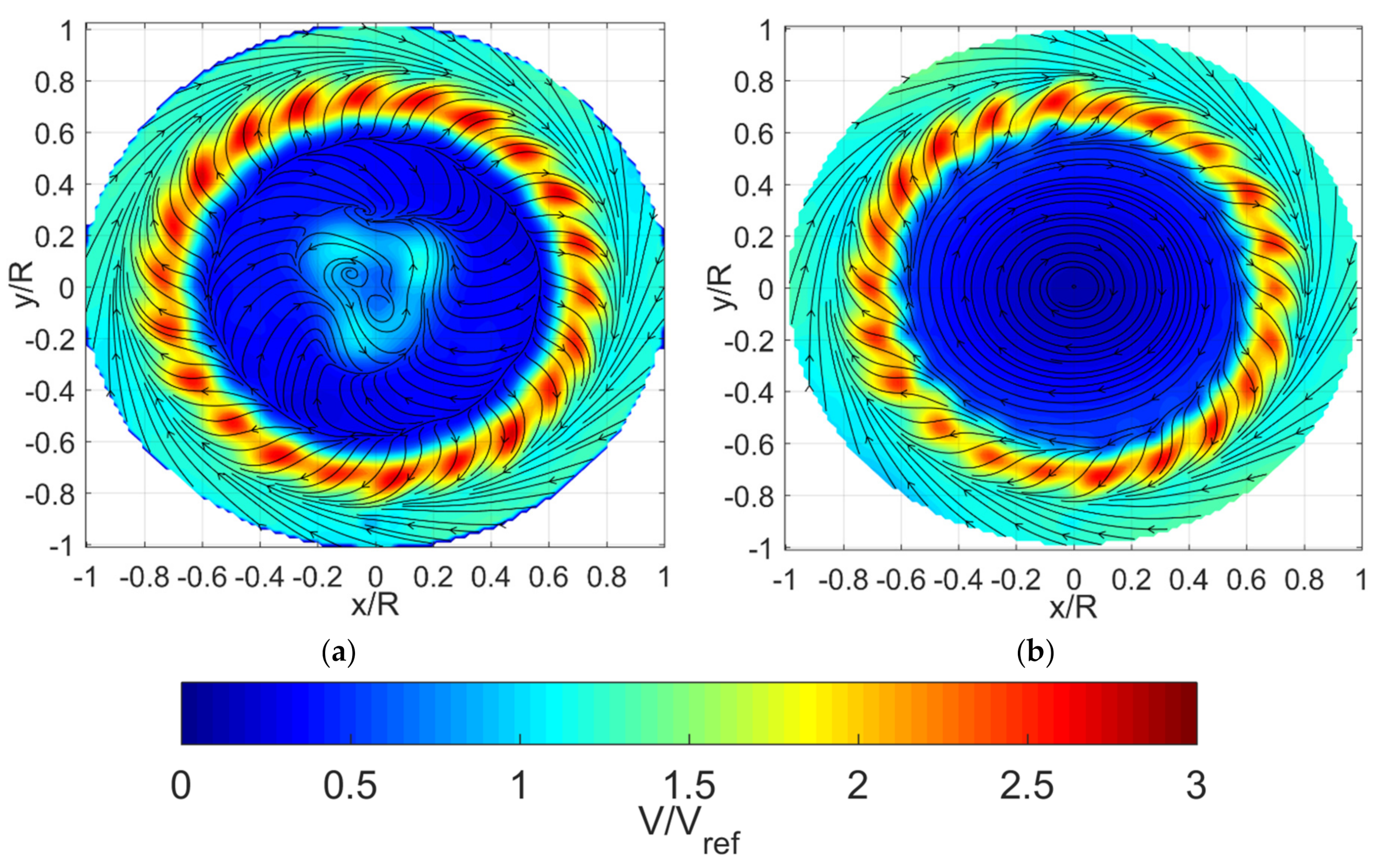
3. Comparisons of Ensemble Average and RMS Distributions

Prior to analysis by proper orthogonal decomposition, insights into the flow characteristics may be found by studying the ensemble average and velocity statistics. Figure 3 presents the ensemble average velocity magnitude and in-plane streamlines of the in-plane components for both injectors.

The two injectors exhibit many common flow features as would be expected given the similarity of their design; the most notable difference being the presence of a central flow structure, associated with the pilot flows in Injector A, Figure 3a. Inside of the mains flow, i.e., R/R_ref < 0.5, a stronger swirl may be observed in Injector B due to the absence of the counter-rotating INT stream.

In understanding the flow characteristics, caution should be exercised in consideration of the ensemble average. It would appear from Figure 3a that the pilot flow has a three-pronged structure when this may not be the case. Instead, the ensemble average may be considered together with the distribution of RMS presented in Figure 4. Considering the pilot region of Injector A (Figure 4a), there is high RMS in this region. This is indicative of either high turbulence in this region and/or the propensity for the bulk pilot stream to move significantly. A better interpretation of the mean flow field in the central region is that it is a locus of preferred locations of the pilot jet, which transits around this triangular locus at relatively low and variable frequency. A visual analogy could be the pilot as a clapper within a bell (the swirl cone) having three regular striking points. For further insight, an estimation of the turbulence will be considered following decomposition later.

The area corresponding to the mains flow (the swirl cone) in both injectors have very similar structures. The jet from these streams is characterized by two peaks of RMS which each indicate the edges of the stream, albeit with lower normalized magnitude.

Furthermore, the locations of these features may be more easily quantified by considering the circumferentially averaged profiles of mean and RMS velocities as presented in Figure 5a,b respectively.

Firstly, the profile of mean velocity shows the same peak normalised velocity through the common passages (MIS and MOS). Because the mass flow rate between the tests carried out on Injector A and Injector B have been appropriately scaled, the nominal absolute velocities are also equal, resulting in the calculation of the same passage-based Re. However, the peak location has shifted inboard for Injector B by 0.02R/R_ref, i.e., 2% compared to Injector A. This is further confirmed in Figure 5b with a similar shift inboard for Injector B. The general RMS profile trend is highly similar over the region of the mains streams, with a notable additional peak in the pilot streams’ region for Injector A as discussed earlier. However, there is also an increased RMS in the region ~0.25–0.55 in the case of Injector A, showing evidence of pilot–mains interaction. The topology of the mains streams may be assessed from Figure 5 and these are summarized in

Table 1. Summary of mains region jet geometric properties (normalized as R/R_ref).

	Inner Edge	Outer Edge	Width
Injector A	0.665	0.780	0.115
Injector B	0.645	0.755	0.110

, where the edges of the mains streams’ flow is defined by the location of the peak circumferentially averaged velocity RMS.

As the mains passages of the injectors remains consistent between the two injector designs, similar flow structures in these areas would be expected, other than the slight shift inboard of Injector B previously discussed. Figure 6 presents only the ensemble average axial velocity in the mains region for each injector, with a radial offset as appropriate according to the inner edge location defined in Table 1, and transformed to polar co-ordinate space. In both injectors, there is clear evidence of the wakes related to the from flows over each MIS/MOS passage vanes. The delta between them, presented in Figure 6c, shows that once the 2% radial offset is accounted for, the two injectors have highly similar characteristics.

4. Analysis by Proper Orthogonal Decomposition

The procedure for POD has been widely published and is briefly described earlier in this paper. This section will deal with the application of POD to the entire (non-masked) spatial domain, as would normally be the approach taken, and then with the ZPOD approach. Finally, spatial modes from both approaches are used to reconstruct the low-order modelled velocity fields.

4.1. Comparison of Injectors’ POD Modes

POD analysis was carried out on each of the injectors’ velocity datasets using the conventional approach. Features of the POD modes are discussed in this section, with reconstructions of the velocity fields from all discussed approaches presented and compared later.

For brevity, a selection of the early POD spatial modes is presented in Figure 7. Visually, the two sets of POD modes have significantly different structure. The first mode (Figure 7a) for Injector A features predominantly structures relating to flow from the pilot streams, with very weak content in any other region of the domain. However, from mode 2 onwards—shown here are mode 2 and 10, Figure 7c,e respectively—the modes contain significant content from both the mains and pilot regions.

This may be directly contrasted with the characteristics of the spatial modes generated from Injector B. Here, all the early modes contain only significant energy contributions within the mains regions. This is as would be expected when considering the ensemble average and RMS velocities associated with this injector (Figure 3b and Figure 4b, respectively), where there is relatively little content in either magnitude or fluctuating velocity outside of the mains region.

The inclusion of structures from each region in the case of Injector A means that more modes are required to capture and represent this information. This can be seen when considering the trend of cumulative energy for the two injectors, presented in Figure 8. For Injector B, fewer modes are required to contain a larger proportion of the energy; in contrast, more Injector A modes have similar levels of energy, leading to a slower rate of change in gradient in the cumulative energy curve.

As well as analysis of the spatial modes and energy content, it is possible to gain insight into any frequency content of structures represented by a particular POD mode. Figure 9a,b present the power spectral densities (PSDs) for Injector A and B, respectively. In each of these figures, the PSD has been estimated using Welch’s method [20], implemented in the MATLAB statistical toolbox up to the Nyquist frequency, presented here normalized as the Strouhal number.

The two injectors’ early POD modes have significantly different frequency characteristics. In the case of Injector A (Figure 9a), there is no easily identifiable peak frequency associated with any of the first three POD modes. In contrast, there is evidence of substantial content in the frequency spectra associated with the early POD modes of Injector B (Figure 9b). A peak in both mode 1 and mode 2 for Injector B occurs at the same Strouhal number of St = 0.07. Mode 3 of Injector B does also exhibit a peak, albeit at lower magnitude and not as clear cut, occurring at St = 0.13. The highly similar nature of mode 1 and 2 for Injector 1 suggest some mode pairing or coupling. Considering the shape associated with modes 1 and 2 for Injector B (Figure 7b,d) are highly similar but rotated, the pairing of these is indicative of a set of structures rotating at a constant radial location. This is in contrast to the early Injector A modes with content in the mains region (Figure 7c,e). These modes do not have the same similarity and phase relationship. Suggesting that there are preferred locations for these structures when a pilot flow is present.

An insight into this characteristic can be gained by taking a closer look at the axial component of these first two POD spatial modes, in the region of the mains flow (Figure 10a,b, respectively). Modes 1 and 2 have a similar appearance, but are phase shifted circumferentially, i.e., in the θ direction. Each of the peaks (positive and negative) alternate in the θ direction, with approximately half as many peaks in each of the two modes as there are in the velocity magnitude distribution over the same region, presented in Figure 6b. This indicates that the structures present in these early POD modes are related to the fluctuations between the wakes from each swirl blade in the mains passages. For context and comparison, the same presentation of POD mode is shown for Injector A, 1st POD mode in Figure 10c. As discussed earlier, and as is evident in the overall view for this mode (Figure 7a), there is very little content in this region in the first mode of Injector A.

This distribution of energy content in the case of Injector A makes it difficult to extract meaningful analysis of either stream independently due to having two sources of significant fluctuating energy. In addition, therefore, many of the strong features are coupled with other features when POD modes are generated, potentially increasing the number of modes required to effectively describe the same phenomena, for example in the mains region. However, it is clear that frequency content associated with these features is difficult to extract in the original geometry case, Injector A, while analysis of Injector B shows that this is present.

4.2. Zonal Proper Orthogonal Decomposition

4.2.1. Application of ZPOD

So far in this paper, analysis, including POD has been applied to the entire spatial domain. This conventional approach is widely used and provides useful insight into flow characteristics, as demonstrated in the previous section. However, in cases where flows have multiple distinct features to be analysed, as is the case here, it may be desirable to apply masking to the vector fields prior to carrying out subsequent decomposition techniques such as POD. This may be necessary to allow increased efficiency in the low-order modelling of flow fields.

Figure 3, Figure 4 and Figure 5 show that Injector A may arguably have up to 4 distinct flow regions/regimes: R/R_ref < 0.35, pilot streams flow; 0.35 < R/R_ref < 0.55, intermediate pilot-mains interaction region; 0.55 < R/R_ref < 0.9, mains streams flow; R/R_ref > 0.9 outside of mains flow, the outer recirculation zone. While it may be possible to define the flow in this way, the two most distinct features of the flow occur in the pilot flow and mains flow regions.

Due to the significantly lower content in two of the four regions described, and for simplification, the spatial domain will be split into two zones with some overlap. These will be zone 1, R/R_ref < 0.55, and zone 2, R/R_ref > 0.45. With respect to Equation (3), the chosen two zones j = (1,2), have POD analysis performed independently where x₁ = {x:‖x‖ < 0.55R_ref} and x₂ = {x:‖x‖ > 0.45R_ref}. Using these values, the flow features of interest sit well within each of the respective zones according to the values stated in Table 1. Other than the pre-masking of the velocity fields, POD analysis is carried out in the same manner as the previous section without zoning. The analysis in this section will focus on the POD analysis of Injector A velocity fields as they feature the two distinct regions of fluctuating energy, whereas the velocity fields of Injector B largely have little content in R/R_ref < 0.55. This absence of fluctuating content means that the inner region has little influence over the generation of POD modes as evident for example in Figure 7a; therefore, modes generated in the previous section shall only be needed for Injector B.

4.2.2. Analysis of Spatial Modes

The POD spatial modes obtained from the separate analysis of zones 1 and 2 are presented in Figure 11 for Injector A. To allow for an equivalent comparison, the same modes, 1, 2 and 10, are presented as in Figure 7.

Considering first the structures within zone 1, the shapes of these in the masked analysis are not dissimilar from those obtained in the same zone within POD modes obtained from the complete (non-masked) spatial domain (Figure 7a,c,e). This is due to the velocity fluctuations giving rise to these still represent the majority of energy and thus appear in the early modes. However, there are some differences when comparing the modes obtained from a masked approach, particularly as later modes are considered, for example, mode 10, presented in Figure 11e. In the non-masked approach, these modes have significant contribution from the mains (Figure 7e), which is of course not present in the masked data.

By directly comparing the masked zone 2 POD spatial modes in Figure 11 to those modes generated in the non-masked approach reveals a difference in the flow structures due to the presence of a pilot flow. It would be expected that if the pilot had no influence on the mains flow, then removing this region from the domain before decomposition should result in POD modes similar to Injector B; however, this is clearly not the case, suggesting some effect due to the presence of the pilot flow.

Close observation of the locations of the peaks within Injector A, zone 2; for example mode 10, Figure 11f, shows that these occur in the same locations as those peaks in Injector B (Figure 7a). However, it seems that in each mode, only a small number of these peaks occur in each individual mode.

By splitting the spatial domain into zones prior to decomposition allows for analysis of any frequency content which is localized within each region. In similar fashion to earlier analysis, the PSD has been calculated for the temporal coefficients associated with each region in Injector A. This is presented in Figure 12. Firstly, it may be observed that the power density in each of the two plots is significantly reduced in comparison to the clear, strong frequency content contained in Injector B POD modes Figure 9b. However, in the case of region two, some low frequency content can be seen, with a similar Strouhal number to the peaks of Injector B early POD modes. However, this covers a broader range of frequencies, suggesting that the structures to which these relate may be disturbed by the presence of a pilot flow. The same analysis carried out on zone 1, shows that there is no significant or clear frequency content within the POD modes associated with this zones flow.

4.3. Reconstruction of Velocity Fields

Much of the analysis to this point has focused on POD spatial modes and temporal coefficient data, but each of the POD mode sets, either POD/ZPOD techniques can of course be used to generate estimates or reconstructions of the time series velocity data. As previously mentioned, the interest lies in Injector A due to the energy and structure distribution in this field and therefore much of the focus of this section will be on that injector. Some reconstructions from Injector B are also presented.

Reconstructions using POD and ZPOD will be carried out using a common number of modes between them. In the case of ZPOD, zone 1 modes will be used to reconstruct R/R_ref < 0.5, and zone 2 to construct R/R_ref > 0.5. There does exist a small overlap region, 0.45 < R/R_ref < 0.55, which will be considered in some of the analysis presented.

The cross-correlation method introduced by Butcher and Spencer [18] shall be used here to select the number of modes used for reconstruction of the velocity fields from the POD spatial modes and temporal coefficients. The technique is described in detail in [18], but the key points shall be outlined here for convenience. The velocity fields captured for Injector B are randomly ordered and split into two equal size sets. The POD spatial modes for each set are calculated separately, resulting in two sets of spatial modes. Given that the early modes should contain only the coherent motions, and the later modes containing stochastic features, the two sets are compared mode by mode via cross-correlation. This allows a single score for each mode which is presented in Figure 13. In line with [18], the cut-off is taken when the score falls below 0.5. For the case presented here, that is mode 12; therefore, all velocity field reconstructions in this section shall be based on the first 12 modes.

It is possible to use the cross-correlation method separately for each set of spatial modes to optimize. However, the purpose of this section is to compare content when the same number of modes is used for each dataset, and therefore the same cut-off is used consistently as described.

As the dataset for Injector A contains 1200 time-steps; it is not efficient nor necessary to present each of the velocity fields. Here, a single timestep example is used to visualize the result of using either method and the information available in each case. Furthermore, whole dataset-level statistics are used to summarize.

The reconstruction of the three datasets for Injector A; POD, ZPOD of zone 1 and ZPOD of zone 2 are presented together for comparison with the original SPIV velocity field in Figure 14 for a single, instantaneous timestep.

Firstly, what is apparent is the filtering/smoothing of small structures that occurs from using the POD technique. This allows the larger and coherent structures to be visualized more easily. Comparing the SPIV and POD velocity fields, Figure 14a,b, respectively, it is evident that the pilot shape is significantly different in the POD reconstruction. While the pilot in the POD velocity field has been altered from the mean flow structure by the early POD modes, it is still not the same broad shape as in the SPIV velocity field.

Conversely, considering ZPOD zone 1 (Figure 14c), the pilot shape is now much closer to the SPIV data. This can be explained by and is a motivation of the ZPOD technique. Using the same number of modes (12), but only to describe the pilot region as opposed to the whole domain, it is reasonable to assume the structure will be closer to SPIV data. For the ZPOD zone 2 data (Figure 14d), there does not appear to be a visible difference between the shapes ZPOD and POD data, but there is a small reduction in magnitude in the mains flow region visible.

Using the velocity distributions presented in Figure 14, and circumferentially averaged profile is extracted and shown in Figure 15a. Both POD and ZPOD lines reasonably estimate the SPIV line, with ZPOD performing better in regions such as the edge of the pilot and within the mains region. The differences between these, i.e., the residual velocity field is evaluated over the whole timeseries and the average is presented in Figure 15b.

Comparing the absolute residuals allows the regions of velocity that are not well represented in the POD/ZPOD reconstructions to be identified. This appears similar in shape to the RMS distribution profile discussed earlier Figure 4a. This is expected as the areas which will not be well represented on an instantaneous basis by common low-order models are regions of high fluctuation. Figure 16 presents the RMS distributions for SPIV, POD and ZPOD, respectively, where the ZPOD is combined ZPOD zone 1 and 2 as appropriate and indicated by the dotted line.

As should be expected, the highest RMS is present in the SPIV data, as any POD approach filters some fluctuating content. However, the differences between the POD and ZPOD RMS distributions reveal an insight to the nature of the RMS. Remembering that both approaches use 12 modes (from a possible 1200), the ZPOD contains more RMS or velocity fluctuations. These fluctuations are typically from several sources: experimental noise/spurious vectors, turbulence or movement of the large-scale structures.

Firstly, the same underlying velocity set is used for POD and ZPOD, and therefore any spurious data would be present in both, and this is typically filtered by excluding the highest order modes. Turbulence is also contained within the higher order modes, and excluded in this approach by using the cross-correlation technique [18]. Therefore, the difference is the capturing of the movement of large structures, i.e., the pilot flow streams as a whole. This agrees with the location of peak RMS and the discussion in Figure 14. This reveals that a significant proportion of the RMS in the pilot region actually comes from an unsteady large structure.

5. Conclusions

This paper presented the analysis of the near-field flow of a lean-burn gas turbine injector. Stereo-PIV was performed on two similar injector models with and without blocked central passages at a parallel plane close to the outlet to obtain three-component velocity distributions. Analysis on this data was carried out using proper orthogonal decomposition, POD and a modified approach, Zonal POD, ZPOD to reveal characteristics of the flow field. The findings of the work can be summarized as the following:

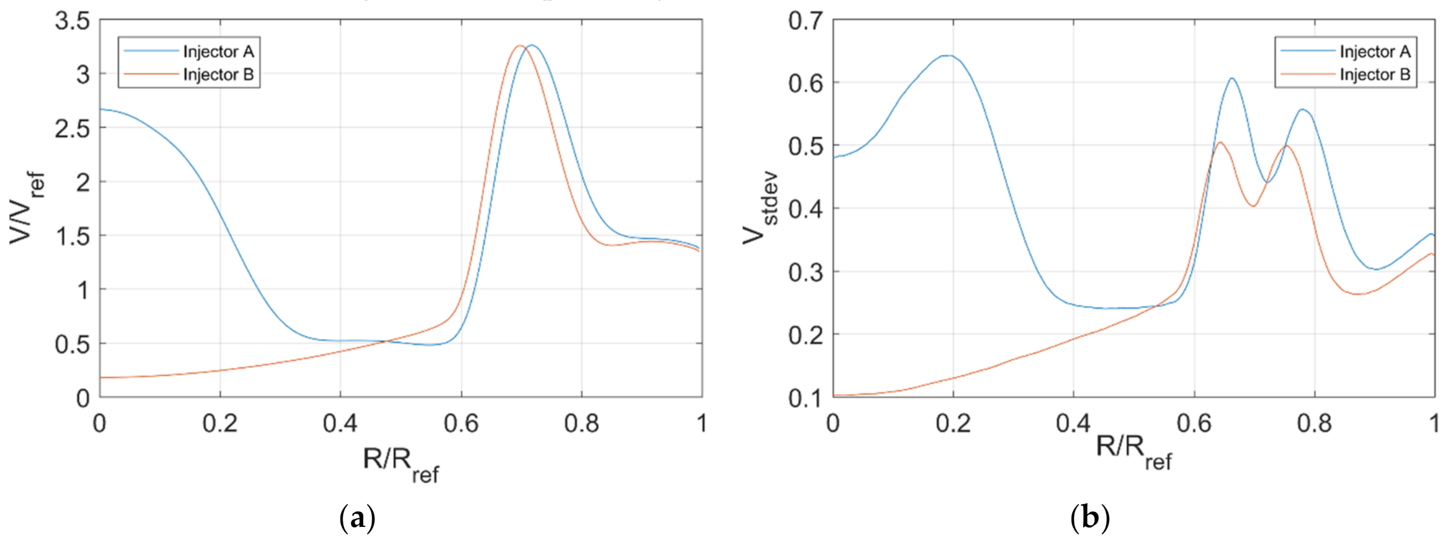
• The mains flow (outer swirl stream) of the two injectors were largely similar in distribution of average velocity, with the five-stream injector (Injector A) showing a 2% radial shift in peak magnitude location compared to the two-stream case (when the inner swirl streams are blocked). However, the RMS distribution reveals an increased magnitude associated with the mains flow in Injector A. The central region, R/R_ref < 0.6 has significant different mean and RMS velocity characteristics due to the presence of the central pilot. Not only does the pilot flow itself have increased magnitude and RMS, but the intermediate region between this and the mains has increased RMS in comparison to the corresponding region for Injector B.
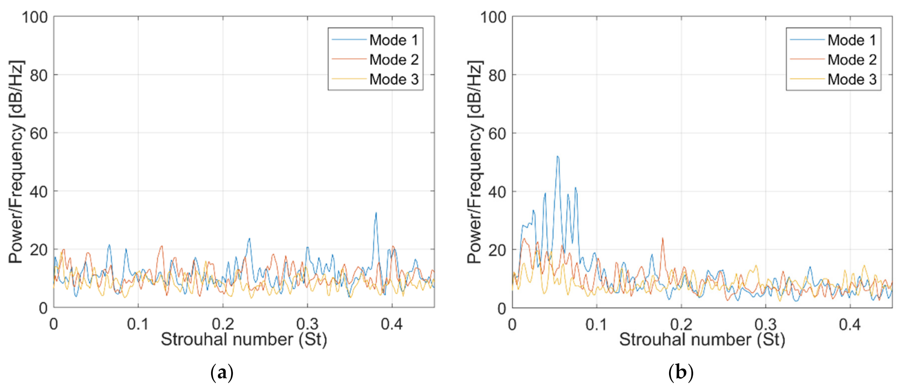
• Analysis of POD spatial modes showed that early modes for Injector A featured structures both from the mains and pilot regions, making it difficult to assess characteristics associated with each. Frequency analysis of Injector B revealed an early mode (i.e., high energy) peak of St = 0.07 associated with rotating structures related to the mains flow. The presence of a pilot flow in Injector A interrupts this feature.
• Application of ZPOD allowed the regions of the flow field to be analysed separately, thereby identifying only the relative energy content of the structures present in each. Applying this to the mains region revealed some frequency content in the same region as in Injector B (St = 0.07); however, the peak was not as clear or strong in this injector.
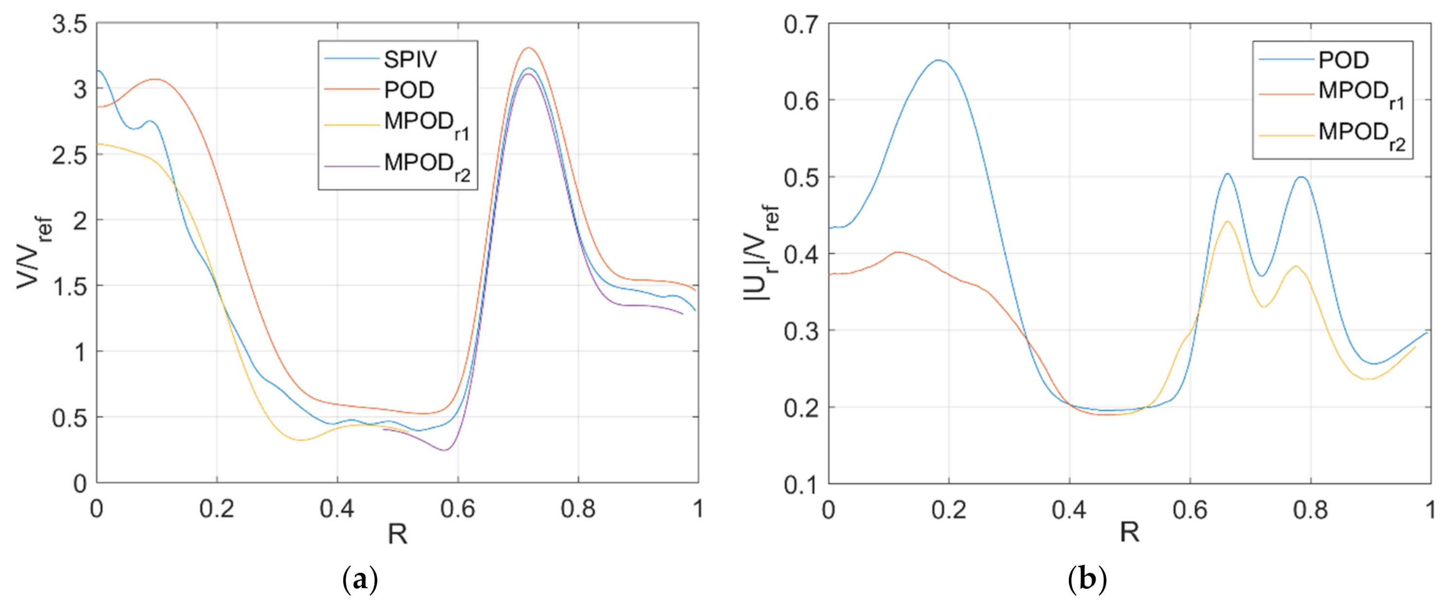
• Further analysis using ZPOD of the pilot region showed that there was significant velocity fluctuation/RMS content associated with large scale movement of the coherent structures. This was not revealed in POD analysis due to the energy ranking of structures associated with two distinct prominent features in the same set, i.e., the mains and pilot jets. Capturing this behaviour in ZPOD modes resulted in reconstructions that were closer to the SPIV data for a given number of low-order spatial modes.
• Finally, by pre-masking the data prior to application of decomposition techniques, a more efficient representation of the SPIV data was obtained. By using the same number of spatial modes in the reconstruction, a more representative vector field was obtained with ZPOD compared with POD.

References

1. Lefebvre, A.H. Gas Turbine Combustion, 2nd ed.; Taylor & Francis: London, UK, 1999. [Google Scholar]
2. Gupta, A.K. Gas turbine combustion: Prospects and challenges. Energy Convers. Manag. 1997, 38, 1311–1318. [Google Scholar] [CrossRef]
3. Beèr, J.M.; Chigier, N.A. Combustion Aerodynamics; Applied Science Publishers: London, UK, 1972. [Google Scholar]
4. Syred, N.; Beèr, J.M. Combustion in swirling flows: A review. Combust. Flame 1974, 23, 143–201. [Google Scholar] [CrossRef]
5. Lin, Y.; Lin, Y.Z.; Liu, G.E. Unsteady flow structures of a counter-rotating swirl cup. In Proceedings of the 45th AIAA/ASME/SAE/ASEE Joint Propulsion Conference & Exhibit, Denver, CO, USA, 2–5 August 2009; pp. 1–7. [Google Scholar] [CrossRef]
6. Schildmacher, K.U.; Koch, R. Experimental investigation of the interaction of unsteady flow with combustion. J. Eng. Gas Turbines Power 2005, 127, 295–300. [Google Scholar] [CrossRef]
7. Spencer, A.; Brend, M.; Butcher, D.; Dunham, D.; Cheng, L.; Hollis, D. Tomographic PIV in the Near Field of a Swirl-Stabilised Fuel Injector. In Proceedings of the ASME Turbo Expo 2018: Turbomachinery Technical Conference and Exposition, Volume 4A: Combustion, Fuels, and Emissions, Oslo, Norway, 11–15 June 2018. [Google Scholar] [CrossRef]
8. Freitag, S. Experimental investigations of fuel preparation in a swirling airflow under realistic conditions without reaction in a combustor model with a point fuel source. CEAS Aeronaut. J. 2018. [Google Scholar] [CrossRef]
9. Westerweel, J.; Scarano, F. Universal outlier detection for PIV data. Exp. Fluids 2005, 39, 1096–1100. [Google Scholar] [CrossRef]
10. Lumley, J.L. The Structure of Inhomogeneous Turbulent Flows. In Atmospheric Turbulence and Radio Wave Propagation; Nauka: Moscow, Russia, 1967; pp. 166–178. [Google Scholar]
11. Taira, K.; Brunton, S.L.; Dawson, S.T.M.; Rowley, C.W.; Colonius, T.; McKeon, B.J.; Schmidt, O.T.; Gordeyev, S.; Theofilis, V.; Ukeiley, L.S. Modal analysis of fluid flows: An overview. AIAA J. 2017. [Google Scholar] [CrossRef] [Green Version]
12. Sirovich, L. Turbulence and Dynamics of Coherent Structues. Part I: Coherent Structures. Q. Appl. Math. 1987, 45, 561–571. [Google Scholar] [CrossRef] [Green Version]
13. Berkooz, G.; Holmes, P.; Lumley, J.L. The proper orthogonal decomposition in the analysis of turbulent flows. Annu. Rev. Fluid Mech. 1993, 25, 539–575. [Google Scholar] [CrossRef]
14. Adrian, R.J.; Christensen, K.T.; Liu, Z.-C. Analysis and interpretation of instantaneous turbulent velocity fields. Exp. Fluids 2000, 29, 275–290. [Google Scholar] [CrossRef]
15. Pavia, G.; Passmore, M.A.; Varney, M.; Hodgson, G. Salient three-dimensional features of the turbulent wake of a simplified square-back vehicle. J. Fluid Mech. 2020. [Google Scholar] [CrossRef]
16. Raiola, M.; Discetti, S.; Ianiro, A. On PIV random error minimization with optimal POD-based low-order reconstruction. Exp. Fluids 2015, 56. [Google Scholar] [CrossRef]
17. Brindise, M.C.; Vlachos, P.P. Proper orthogonal decomposition truncation method for data denoising and order reduction. Exp. Fluids 2017, 58, 28. [Google Scholar] [CrossRef]
18. Butcher, D.; Spencer, A. Cross-correlation of POD spatial modes for the separation of stochastic turbulence and coherent structures. Fluids 2019, 4, 134. [Google Scholar] [CrossRef] [Green Version]
19. Butcher, D.; Spencer, A.; Chen, R. Influence of asymmetric valve strategy on large-scale and turbulent in-cylinder flows. Int. J. Engine Res. 2018, 19, 631–642. [Google Scholar] [CrossRef] [Green Version]
20. Welch, P.D. The Use of Fast Fourier Transform for the Estimation of Power Spectra: A Method Based on Time Averaging Over Short, Modified Periodograms. IEEE Trans. Audio Electroacoust. 1967. [Google Scholar] [CrossRef] [Green Version]
Figure 1. Schematic of vertical water flow test facility.
Energies 14 01789 g001
Figure 2. Schematic of injectors A and B (left and right half, respectively). The geometry is indicative, and some features have been omitted and/or obscured.
Energies 14 01789 g002
Figure 3. Ensemble average normalized in-plane velocity distribution with in-plane streamlines for: (a) Injector A; (b) Injector B.
Energies 14 01789 g003
Figure 4. RMS of normalized velocity magnitude for: (a) Injector A; (b) Injector B.
Energies 14 01789 g004
Figure 5. Circumferentially averaged profiles of: (a) Normalized mean velocity magnitude; (b) RMS of normalized velocity magnitude.
Energies 14 01789 g005
Figure 6. Average axial velocity in mains region for: (a) Injector A; (b) Injector B; (c) Absolute difference between (a) and (b).
Energies 14 01789 g006
Figure 7. POD spatial modes magnitude for: (a) Injector A 1st; (b) Injector B 1st; (c) Injector A 2nd; (d) Injector B 2nd; (e) Injector A 10th; (f) Injector B 10th.
Energies 14 01789 g007
Figure 8. Cumulative mode energy for injectors A and B (truncated at 100 modes).
Energies 14 01789 g008
Figure 9. Early modes’ frequency power spectrum for: (a) Injector A; (b) Injector B.
Energies 14 01789 g009
Figure 10. Zoomed view of axial component of POD spatial modes: (a) Injector B, 1st mode; (b) Injector B 2nd mode; (c) Injector A 1st mode.
Energies 14 01789 g010
Figure 11. POD spatial modes magnitude for: (a) Zone 1, 1st mode; (b) Zone 2, 1st mode; (c) Zone 1, 2nd mode; (d) Zone 2, 2nd mode; (e) Zone 1, 10th mode; (f) Zone 2, 10th mode. All Injector A (Note change in scale).
Energies 14 01789 g011
Figure 12. Early modes’ frequency power spectrum associated with mask POD data for Injector A: (a) Zone 1; (b) Zone 2.
Energies 14 01789 g012
Figure 13. Correlation value for Injector B POD spatial modes.
Energies 14 01789 g013
Figure 14. Comparison of instantaneous velocity fields for: (a) SPIV result; (b) POD using whole region; (c) ZPOD using zone 1; (d) ZPOD using zone 2. In (bd), the first 12 modes are used, and the same time, t1, is used for all sub-figures.
Energies 14 01789 g014
Figure 15. Comparison of normalized circumferentially averaged velocity profiles for: (a) Velocity magnitude for instantaneous time, t1; (b) Average residual over time-series (vs. SPIV).
Energies 14 01789 g015
Figure 16. Distribution of RMS velocity for: (a) SPIV; (b) POD; (c) ZPOD; where R < 0.5 from zone 1, R > 0.5 from zone 2, denoted by dotted line. (b,c) Reconstructions use the first 12 modes.
Energies 14 01789 g016