Article

Experts versus Algorithms? Optimized Fuzzy Logic Energy Management of Autonomous PV Hybrid Systems with Battery and H2 Storage

Chair of Energy Storage Systems, Technische Universität Dresden, Helmholtzstraße 9, 01069 Dresden, Germany
*
Authors to whom correspondence should be addressed.
Energies 2021, 14(6), 1777; https://doi.org/10.3390/en14061777
Submission received: 15 February 2021 / Revised: 16 March 2021 / Accepted: 18 March 2021 / Published: 23 March 2021

Abstract

:
Off-grid applications based on intermittent solar power benefit greatly from hybrid energy storage systems consisting of a battery short-term and a hydrogen long-term storage path. An intelligent energy management is required to balance short-, intermediate- and long-term fluctuations in electricity demand and supply, while maximizing system efficiency and minimizing component stress. An energy management was developed that combines the benefits of an expert-knowledge based fuzzy logic approach with a metaheuristic particle swarm optimization. Unlike in most existing work, interpretability of the optimized fuzzy logic controller is maintained, allowing the expert to evaluate and adjust it if deemed necessary. The energy management was tested with 65 1-year household load datasets. It was shown that the expert tuned controller is more robust to changes in load pattern then the optimized controller. However, simple readjustments restore robustness, while largely retaining the benefits achieved through optimization. Nevertheless, it was demonstrated that there is no one-size-fits-all tuning. Especially, large power peaks on the demand-side require overly conservative tunings. This is not desirable in situations where such peaks can be avoided through other means.

1. Introduction

Residential off-grid applications relying on intermittent renewable sources for their energy supply benefit greatly from hybrid energy storage systems. The integration of storage technologies with supplementary operating characteristics allows an efficient and economic balancing of short-, intermediate- and long-term fluctuations in electricity demand and supply [1].
A particularly promising topology consists of lithium-ion batteries combined with a hydrogen (H2) storage path. H2 systems, comprising an electrolyzer, a H2 tank and a fuel cell, are especially suited for medium- to long-term storage, and can be employed to compensate seasonal fluctuations. H2 has a high energy density, and the system capacity is solely dependent on tank size [2]. On the other hand, both electrolyzer and fuel cell suffer from excessive strain if exposed to fast power dynamics. Pressure imbalance, flooding of cells, fuel starvation and membrane drying lead ultimately to stack degradation [3]. By letting lithium-ion batteries cover power peaks and fast fluctuations, the H2 components can be kept close to their optimal operating region, resulting in lower losses and reduced degradation [1]. The combination of high-energy with high-power storage devices is also beneficial from an economic point of view [1,4,5]. By decoupling energy and power, the high-energy storage device, which has a relatively low capacity cost, covers the average power demand only, while the high-power storage device, which is comparatively cheap in terms of cost per kW, can be designed with a smaller capacity.
To reap the full range of benefits offered by such a system, an intelligent energy management is required [6]. It controls the power flows aiming at maximizing overall efficiency, while minimizing component stress. According to [1], it is possible to categorize control strategies for hybrid storage systems into rule-based and optimization-based approaches. Rule-based algorithms are particularly suited for real-time applications. In off-grid systems, where power demand and supply are subject to stochastic fluctuations, and where there is no aggregation of load profiles, real-time capability is an important property, as power flows need to be balanced at any given point in time to guarantee system stability [7]. The most elementary and probably most common rule-based control strategy is based on a three-point hysteresis controller. The fuel cell and the electrolyzer are switched on and off according to a lower respectively upper threshold of the battery state of charge (SOC) [8,9]. There are several disadvantages to this approach. Firstly, the electrolyzer and the fuel cell are operated in one fixed point even if other operation regions may be more suitable. Secondly, the control decisions are solely based on the battery’s SOC, thus ignoring other system states [9,10]. These shortcomings can be overcome by adopting fuzzy logic in the decision making. The main benefits of a fuzzy logic controller are its intuitive design based on expert knowledge, the possibility for multiple inputs and multiple outputs—allowing incorporation of different system states in the control decisions—and the calculation of continues reference values [1,9,10,11].
A number of past works have applied fuzzy logic control to off-grid systems with batteries and H2 storage path [2,11,12,13,14,15]. In these applications the SOC of the battery and a representation of the net power flow are used as inputs to the fuzzy logic controller, which then provides a power reference to the H2 storage path. In order to broaden the perspective, further studies using fuzzy logic control in comparable applications were reviewed. They all have in common that the net power flow is to be divided between a short-term storage system—in most cases a battery—and a storage system or power source covering intermediate- and long-term load fluctuations. These include off-grid PV battery diesel [16,17,18,19,20] or fuel cell systems [21], and battery fuel cell hybrid energy storage systems in electric vehicles [4,5,22]. Moreover, in [23,24] batteries are used to smoothen grid power injection with the help of a fuzzy logic controller. In this case, the grid can be considered a long-term storage system with infinite capacity. Fuzzy logic control is also employed in grid-connected battery hydrogen systems. However, they are of lesser relevance to this work, as the degrees of freedom and main objectives are markedly different [25,26,27].
Whereas the fuzzy logic controller’s intuitive design is one of its very strength, it leads also to drawbacks. The underlying expert knowledge is generally not reported in enough detail to make external evaluation possible. Indeed, the tuning appears often to be a trial and error process based on some simulation model [28]. This is a disadvantage, given that the fuzzy rule base and the parametrization of membership functions have a large influence on the controller’s performance. Furthermore, even if comprehensive expert knowledge is used for tuning, it will likely result in a good but not in an optimal energy management system. Hence, it is not surprising that the tuning of rules and membership functions has been combined with several different, mostly heuristic, optimization methods, such as genetic algorithms, particle swarm algorithms, cuckoo search algorithms etc. [5,15,19,20,21,23,24,29]. In these cases, though, the interpretability of the resulting fuzzy logic controller is lost. Consequently, an optimal tuning can only be guaranteed for the specific case it has been trained for. Considering that the availability of large amounts of historic data is often not given, the lack of generalizability is problematic. Reviewing above articles, including both articles with and without optimized fuzzy logic controllers, revealed that the data basis for evaluation is generally very narrow. Usually, a single data set of a few days to maximum 1 year is used for verification. This raises question about validity.
Summarizing, three main research gaps were identified: Firstly, the underlying expert knowledge linked to the configuration and tuning of fuzzy logic energy management is not presented in sufficient detail, making evaluation and comparison difficult. Secondly, applying metaheuristic algorithms for optimization leads generally to a loss of interpretability, which is considered one of fuzzy logic’s main strengths and thirdly, the verification of fuzzy logic energy management is based on very limited data sets, not accounting for the large variety found in load and generation profiles. Hence, validity of simulation results is often limited. These gaps are likely to hamper a joint and cumulative development of fuzzy logic control for the energy management of hybrid energy storage systems.
Therefore, this article makes the following contributions: Firstly, it aims at giving a detailed account of the expert knowledge used to design the fuzzy logic controller in the context of autonomous PV hybrid systems with battery and H2 storage path. Secondly, a particle swarm optimization is adapted to tune both the rule base and the membership functions of the fuzzy logic controller without losing interpretability of the outcome. Thirdly, the manually and the optimized fuzzy logic controller is tested with data from 65 households to verify both robustness and generalizability of results. Lastly, the favorable interplay between expert knowledge and optimization, which is made possible by contributions one to three, is illustrated.
The remaining of the article is structured as follows: Section 2 presents the system configuration of an autonomous PV hybrid system and the resulting implications for the energy management. Section 3 provides the theoretical basis of fuzzy logic control applied to the energy management of hybrid storage systems and discusses the controller structure as well as the tuning methods. Section 4 describes the simulation framework and the database. Section 5 presents the simulation study including the discussion of results, and Section 6 concludes the paper giving an outlook for further research.

2. System Topology and the Energy Management Problem

The system topology, the energy management problem, and its overall objectives are closely connected and will be shortly discussed in the following section.

2.1. System Topology

The favorable characteristics of hybrid energy storage systems combining batteries with a H2 storage path in PV-off-grid applications have been pointed out by [1]. Especially for locations with seasonal variations in solar irradiation, the H2 storage path can be used advantageously to balance seasonal excess and deficit, whereas the battery is apt to compensate short-term fluctuations in both PV-supply and load. Furthermore, the battery can be used to optimize the efficiency of fuel cell and electrolyzer and at the same time, reduce component degradation by avoiding unfavorable operation points, frequent switching and dynamic stress. From a cost perspective, the configuration is favorable, as the overall installation cost for the H2 storage path is dominated by the cost per installed power, while the cost structure of the battery is dominated by its capacity. Hence, by combining a H2 storage path with low power and high capacity and a battery with high power, but low capacity the overall cost can be considerably reduced.
There are several possibilities to connect the individual components to form the off-grid system. For the example used in this paper all components are coupled via a central DC-bus. The PV system, the electrical load, the lithium-ion battery and the H2 storage path are connected to the bus with a converter each (see Figure 1). Power flows entering the central DC-bus are defined positive, while power flows leaving the central DC-bus are defined negative.

2.2. Energy Management: Problem Structure and Objectives

There are a number of control tasks that need to be performed in order to allow the operation of an off-grid system. A common way to structure these tasks is to define hierarchical control layers whose dynamics are decoupled as a result of time scales which are separated by at least one order of magnitude [1,30]. In the context of this work, a primary control layer, taking care of the voltage and current control, and an energy management layer are defined. The primary control is performed by the converters and has response times between 1 ms to 1 s. The battery converter maintains the bus voltage, whereas all other converters in the system are current led [3]. The set points of the latter are assigned by the energy management system which controls the power flows in the system. The energy management operates in a discrete manner in the order of seconds to hours [30]. The primary control and the energy management system can be analyzed and designed separately, as long as the SOC of the battery is maintained at sufficient levels. The focus in this article is on the energy management system only.
The overarching objective of the energy management is to guarantee security of supply, i.e., to make sure that the energy storage systems can balance differences in power generation and demand at all times. Given the sign convention defined in Section 2.1, this can be achieved by satisfying the power balance as expressed in Equation (1). It is assumed that excess PV power P P V , c u r t can be curtailed for example with a dump load. The rationale behind such an action is explained later in this section. On the other hand, load shedding is only to be used as last resort in case of unexpected events or failures and has therefore not been added to the equation.
P P V + P P V , c u r t + P L o a d + P F C + P E L + P B a t t = 0
Beyond this, there are two secondary objectives: high system efficiency and low degradation of electrolyzer and fuel cell. In this context, two cases need to be differentiated: Firstly, the design of an improved energy management for an existing system, and secondly, the design of an energy management for an entirely new system. In the former case, the hardware with its corresponding power and capacity ratings is given. Assuming unchanged demand, increased efficiency will result in energy surplus, i.e., excess H2. To some extent, this can increase security of supply. However, if no additional energy is needed, the increase in efficiency does not result in an added benefit. Hence, there should be a focus on increasing component lifetime to defer reinvestment. For a new system, a co-design of component sizes and control approach is possible and desirable [31,32]. Increased efficiency allows smaller sized components, saving costs and resources. These considerations are important, as there will be trade-offs between increased system efficiency and decreased component fatigue. As a result, finding the right balance between objectives calls for a careful analysis of the use case. Notwithstanding, a notion of Pareto optimum can be established, that is an energy management resulting in a higher system efficiency given the same levels of component fatigue (or vice versa) can be considered superior.
The system efficiency results from the efficiency of the individual components and the relative energy throughput. This can be illustrated by the possible paths between PV generation (source) and load (sink) and the corresponding efficiencies as depicted in Equations (2)–(7). The relevant efficiencies are the efficiency of the PV plant η P V , the PV DC–DC converter η D , P V , the battery DC–DC converter η D , B a t t , the battery η B a t t , the electrolyzer DC–DC converter η D , E l , the electrolyzer η E l , the fuel cell η F C , the fuel cell DC–DC converter η D , F C , and the inverter connected to the AC load η I N .
1.
Direct from PV to load:
η 1 = η P V · η D , P V · η I N
2.
Using battery storage:
η 2 = η P V · η D , P V · η D , B a t t · η B a t t · η D , B a t t · η I N
3.
Using H2 storage:
η 3 = η P V · η D , P V · η D , E l · η E l · η F C · η D , F C · η I N
4.
Using battery storage before or after using H2 storage:
η 4 = η P V · η D , P V · η D , B a t t · η B a t t · η D , B a t t · η D , E l · η E l · η F C · η D , F C · η I N
5.
Using battery storage before and after using H2 storage:
η 5 = η P V · η D , P V · η D , B a t t · η B a t t · η D , B a t t · η D , E l · η E l · η F C · η D , F C · η D , B a t t · η B a t t · η D , B a t t · η I N
6.
Curtailing PV power:
η 6 = 0
It can easily be seen that the efficiencies decrease from path 1 to path 6 (Equations (2)–(7)). In consequence, there is a clear order of preference from an efficiency point of view. However, from a more holistic stance, it can be reasonable to oversize the PV plant and accept curtailment if this allows smaller storage components and/or results in less component stress, as PV panels are relatively cheap compared to the storage units.
The battery power is not controlled directly by the energy management system. Rather, it gets its reference from the underlying DC-bus voltage controller, and thus covers any residual power, ensuring security of supply. Therefore, ageing effects from cycling cannot be actively reduced. However, as ageing processes in lithium-ion batteries are accelerated at both very low and very high states of charge [33], preventing operation in these regions is favorable. Furthermore, unnecessary charging and discharging as in power paths 4 and 5 should be reduced.
The electrolyzer and fuel cell can be fended from premature ageing through a number of measures. First of all, limiting the operation range to points below nominal power reduces the probability of unbalanced concentration and current distributions in the cells. Moreover, less steep power gradients avoid fuel starvation, flooding of cells and drying out of the membrane. Finally, corrosion, which results from high potentials at the electrodes, can be reduced by minimizing the number of startups and shutdowns [34]. Whereas fuel cell voltage reduces with ageing, electrolyzer voltage increases [35].
There are clear trade-offs between increasing efficiency and reducing stress on the components. This is, for example, the case if the PV power is curtailed to prevent the battery from operating at too high SOCs, or if power paths 4 and 5 are chosen, despite higher losses, to reduce dynamic stress or switching of fuel cell and electrolyzer. Nevertheless, in many instances increasing efficiency and reducing stress do not contradict each other. For example, if the fuel cell is only operated in those periods where the battery cannot cover the load, the higher efficiencies of the battery are exploited, while fuel cell degradation is avoided.
Summarizing, the energy management system determines the power set points of the electrolyzer as well as the fuel cell and decides if the PV-generation should be curtailed or parts of the load shed. The charging and discharging behavior of the battery is controlled indirectly through the voltage deviations which result from a power mismatch between load and generation. How the set-points of the electrolyzer and fuel cell are to be chosen to fulfil the above discussed objectives is the question to be answered during controller design.

3. Fuzzy Logic Energy Management

The control objectives can be achieved either by choosing an apt controller structure or by finding the right parametrization of the controller. In this section, the theoretical basis of fuzzy logic control is presented, the structure of the fuzzy logic controller defined, the control law designed based on expert knowledge, and the process of optimization discussed. The controller is designed for the topology described in Section 2 and aimed at supplying electricity to a single-family household.

3.1. Fuzzy Logic Control

To provide the reader unfamiliar with fuzzy logic control with a basic understanding, this section shortly describes the very fundamentals of fuzzy logic control that are relevant to the methods used in this article. For a more detailed discussion of the general theoretical background, the reader is referred to the pertinent literature [36,37,38]. As the fuzzy logic controller used in this article is a Mamdani-controller, the discussion is limited to this type.
Fuzzy logic control is based on the notion of fuzzy sets. In fuzzy sets, an element x has a degree of membership—a real number in the interval [ 0 , 1 ] —to a given set A, which is determined according to a membership function μ A ( x ) . This should be seen in contrast to classical set theory, where an object can either be part of a set or not [38,39].
A basic block diagram of a fuzzy logic controller is depicted in Figure 2 [40]. The controller outputs are derived from the controller inputs in three steps. Each input—in the context of this article for example the SOC of the battery—can be considered as a linguistic variable, which can hold different linguistic terms, such as “low”, “good” or “high”. A variable holding a specific linguistic term forms so called fuzzy sets, i.e., “low SOC”, “good SOC” and “high SOC”, which are described each by a corresponding membership function. Using this type of description, a crisp (numeric) value, e.g., SOC = 0.6 , can be associated with each fuzzy set by a corresponding degree of membership. This process is called fuzzification [39].
The second step consists in the fuzzy inference. It uses R If-Then rules, which are provided by the rule base. If-Then rules have the form:
R: If x 1 is μ R ( 1 ) and ... and x n is μ R ( n ) , then y is μ R
The conclusion of the rule, i.e., its degree of fulfilment, depends on the degree of membership of the antecedents, which are combined using the min-operator [41]. Each rule, which is fired, results in a fuzzy set. To get the combined fuzzy set characterizing the output value, an aggregation step follows in which all fuzzy sets are combined with the max-operator. This approach follows the original procedure suggested by Mamdani and Assilian [37].
In a last step, the crisp outputs are derived from the output fuzzy sets by means of defuzzification. The most common method is based on calculating the centre of area ( k C O A ) below the output fuzzy sets and projecting it on the ordinate as shown in Equation (8) [41]. As this method is well suited for overlapping membership functions [42], it was chosen as a good candidate for the fuzzy logic energy management.
k C O A ( μ R o u t p u t ) = Y μ R o u t p u t · y d y Y μ R o u t p u t · d y

3.2. Controller Structure

The energy management system’s inputs and outputs are on the highest level of the controller’s structure. By choosing the battery converter to be voltage led (compare Section 2), all high frequent variation in generation and load, i.e., everything above the sampling rate of the energy management system, is automatically compensated by the battery energy storage. As a consequence, only electrolyzer and fuel cell power are controllable. As these two components will never be operated simultaneously, one control output is sufficient. We should call this P H 2 . If P H 2 > 0 , then P H 2 = P F C and P E L = 0 . If P H 2 < 0 , then P H 2 = P E L and P F C = 0 .
To ensure the stability of the system, the SOC of the battery needs to be kept within certain limits. Only if the battery’s SOC allows both charge and discharge can the battery be used to control the voltage of the DC-bus. Thus, the SOC of the battery is the variable to be controlled by the energy management system and accordingly a control input. One possibility of controlling the SOC is to use the battery to balance any mismatch between generation and load unless an upper or a lower SOC-threshold is reached, in which case the electrolyzer or respectively the fuel cell are switch on until acceptable SOC levels are restored. However, there are at least two disadvantages with this approach: firstly, there is no possibility to actively avoid paths 4 and 5 and secondly, the nominal power of both the fuel cell and the electrolyzer are considerably lower than the minimum and respectively the maximum of P n e t = P P V + P L o a d . Only P n e t is relevant for the control task, as the load is whenever possible directly supplied by the PV panels. This corresponds to path 1 of the power paths discussed in Section 2.2 and is a measure of no regret. Thus, once the battery is fully charged (on a summer day this is likely to happen long before noon), the electrolyzer can only use a small part of the PV power. The remaining PV power needs to be curtailed. Similarly, if the battery is empty, the fuel cell cannot cover the entire demand. Furthermore, using the H2 storage path, losses are considerable. Therefore, it is beneficial to add P n e t as an input to the fuzzy logic controller. From a control perspective P n e t resembles a differential input. If the H2 storage path is not active, the battery’s SOC is the weighted integral over P n e t . Whereas, the battery SOC changes rather slowly, because of its integral characteristic, P n e t provides this information much quicker and unnecessary control action on the part of the H2 components can be avoided. For example, if the battery SOC is high, i.e., the battery should be discharged or at least not charged further, a controller, which only sees the battery SOC as input, would switch the electrolyzer on. However, if P n e t is negative, i.e., there is a power deficit in the system, this is unnecessary as the battery will be discharged anyway. This is particularly relevant in the light of daily patterns of surplus and deficit.

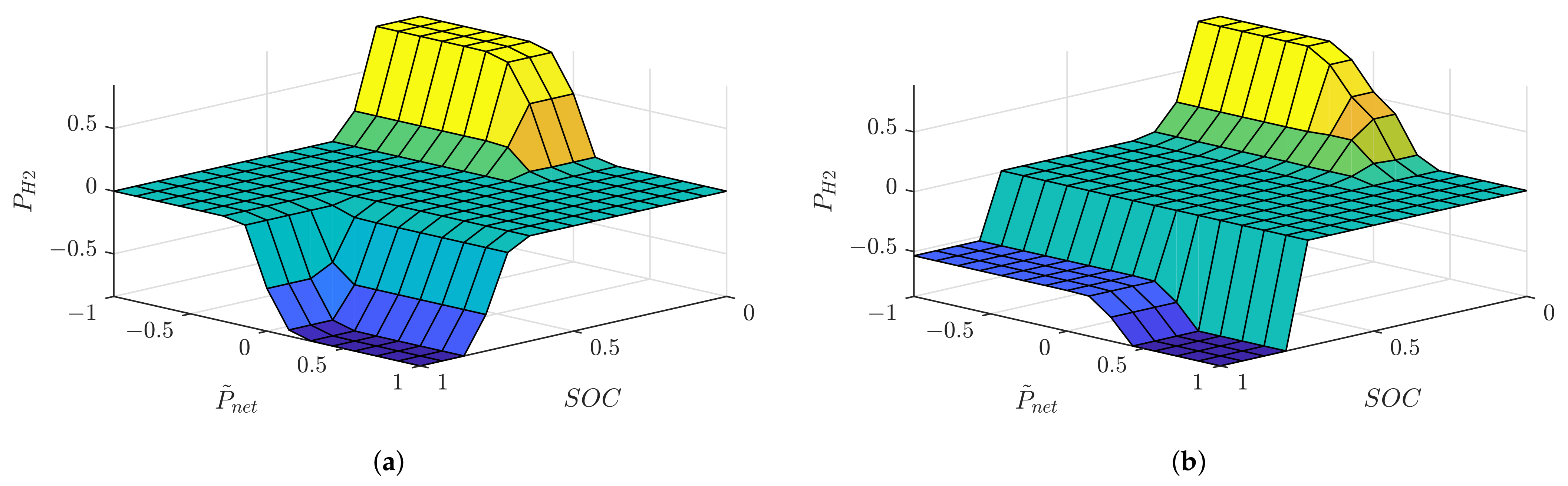
3.3. Definition of Membership Functions

For each in- and output fuzzy set corresponding membership functions need to be designed. The number of fuzzy sets should follow a natural language description, i.e., how would an expert describe the variables. For example, it is natural to think about the SOC of the battery as being low, good or high. Depending on its state different logics for action are applied. If a linguistic category applies equally to a range of values, a trapezoidal membership function is appropriate. If a gradual change with a single maximum is more natural, triangular functions are a good starting point [43,44]. A few design rules help to avoid unintuitive behavior of the control output. First, the whole range of possible values for each variable should be covered by at least one membership function. This ensures that all points in the control surface can be reached and that there are no input values without a conclusive output. Second, the total degree of membership for each crisp value should add up to 1 to avoid discontinuous behavior of the controller. This is achieved if the maximum of one membership function corresponds to the minimum of the next membership function. Following these lines of thought, the membership functions as depicted in Figure 3 were defined. To keep the controller as generic as possible, i.e., independent of component sizes, both inputs and outputs are normalized. The SOC of the battery is by definition normalized on the range [0,1]. P n e t is normalized on a range [−1,1]. P ˜ n e t = 1 corresponds to the peak power of the PV system. The definition of the minimum of P n e t corresponding to P ˜ n e t = 1 is more difficult to define, as the peak load is not known a priori. One possibility is to set it to the connected load, which according to the German norm DIN 18015-3 corresponds to 14.5 kW for a household without electric water heating [45]. The output P ˜ H 2 = 1 corresponds to the maximum power of the electrolyzer and P ˜ H 2 = 1 to the maximum power of the fuel cell.
The lower battery SOC thresholds should be chosen as high as possible to reduce low battery SOCs, which lead to increased battery ageing. In the same vein, the upper battery SOC thresholds should be chosen as low as possible to reduce high battery SOCs. However, choosing these values too conservatively reduces the usable battery capacity. Therefore, the thresholds chosen are 0.15 and 0.25 for the lower limits and 0.7 and 0.8 for the upper limits. P ˜ n e t is considered negative big (NB) for values below 0.3 times the minimum and positive big (PB) above 0.3 times the maximum. The range covered by the fuzzy sets NB and PB are comparatively large in order to account for the fact that the nominal fuel cell and the electrolyzer power are considerable smaller than the minimum/maximum of P ˜ n e t . Hence, from the viewpoint of the control task the power is considered large. The value range of P ˜ H 2 is covered symmetrically by the fuzzy sets. As the crisp fuzzy output never reaches the extreme values but is limited by the centre of area of the outermost fuzzy sets, calculating the actual references from the normalized output is preceded by another scaling, which accounts for this fact.

3.4. Definition of Rule Base

Given the definition of the membership functions the expert knowledge can be easily represented in the rule base. Especially the extreme points are straightforward (see rules 1, 5, 8, 11 and 15 in Table 1). It is the general objective to keep the battery SOC in what is defined as the “good-region”. Only then the full potential of the battery as both a sink and source can be used. In the case of a low SOC and a large deficit in the power balance ( P ˜ n e t is NB), the fuel cell should operate at its maximum, which corresponds to its nominal operation point. However, if there is a large surplus in the energy balance ( P ˜ n e t is PB) the H2 storage path is not needed. Conversely, in the case of a high SOC and a large surplus in the energy balance ( P ˜ n e t is PB), the electrolyzer should operate at its maximum. However, if there is a large deficit in the energy balance ( P ˜ n e t is PB) the H2 storage path is not needed. If the SOC is good, no action is required. The missing rules leave more room for discussion, which will play a role in the optimization. As a starting point, the relationships stated in Table 1 were chosen.

3.5. Particle Swarm Optimization

As mentioned earlier, the idea of optimizing the parameters of a fuzzy logic controller appears quite natural. That way, expert knowledge can be complemented with the results of a search algorithm. The most common used approaches are based on metaheuristics. In this article particle swarm optimization is used as an example. Particle swarm optimization is inspired by mechanisms of social interaction as they appear in flocks of birds and schools of fish [46,47,48]. The particle swarm represents possible problem solutions by means of multidimensional vectors, which are adapted in an iterative fashion. Each dimension of a particle’s position in the solution space x ( n ) represents one parameter that is to be optimized. The particles move through the solution space with a certain velocity v ( n ) , exploring different solution possibilities. The change of a particle n’s velocity is represented by Equation (9) and its position by Equation (10). During every iteration, the particle’s fitness is calculated and its best solution p b e s t as well as the swarm’s global best solution g b e s t are stored.
v ( n ) = v ( n ) + 2 · r a n d · ( p b e s t ( n ) x ( n ) ) + 2 · r a n d · ( g b e s t x ( n ) )
x ( i ) = x ( n ) + v ( n )
In this article a population of 30 particles was chosen, which corresponds to the number used in related work [29,31] and thus is considered a good starting point. As the appropriate number of particles is dependent on the nature of the problem, further investigations into the influence of this parameter are to be carried out in the future [49]. An overview of the tuning procedure based on particle swarm optimization is depicted in Figure 4 as a block diagram and in Figure 5 as the corresponding flowchart. The numbering indicates the link between the two figures.

3.5.1. Fitness Function

The definition of an appropriate fitness function F is crucial for a proper functioning of the particle swarm optimization, as it quantifies the quality of the solution represented by a given particle. To this end, the energy management’s objectives—high system efficiency and reduced component stress constrained by the demand of ensuring security of supply—need to be represented by the fitness function. Likewise, the dataset should be chosen carefully. To include both short- and long-term dynamics, 1-year simulations of the autonomous PV hybrid system are used to evaluate a particle’s fitness (compare Section 4).The energy management’s objectives are operationalized as follows:
  • The system efficiency can be expressed by the overall annual energy losses E l o s s , a —the sum of battery, fuel cell, electrolyzer and PV curtailment losses—which are to be minimized to maximize system efficiency.
  • The component stress on the H2-components can be divided into cyclical stresses, which are operationalized by the number of startups of the electrolyzer N S t a r t , E L and the fuel cell N S t a r t , F C respectively, and degradation that follows normal operation, which is represented by the operation time of the electrolyzer T E L and the fuel cell T F C . N S t a r t , E L , N S t a r t , F C , T E L , T F C are to be minimized.
In order to combine all objectives into one measure of fitness, a weighted sum is used [50]. It is assumed that the weights are chosen by the designer according to the user’s preferences and the specific characteristics of the components. For example, how do cyclical and operational stress relate to each other over the lifetime of the component? How important is an increased energy surplus at the end of the year? To ease the choice of weights, two conventions are used: first, all weights sum to 1, and second, all objective functions f i are normalized.
f i ˜ = f i f i 0 f i m a x f i 0
In our context, the attainable minimum f i 0 is 0 for all objective functions. Hence, the normalized values can be expressed as follows:
f i ˜ = f i f i m a x
The maximum allowed value f i m a x for the system losses is equal to the annual surplus of PV-energy, i.e., the annual PV generation E P V , a minus the annual energy consumption E L o a d , a . The maximum operation duration for the fuel cell and the electrolyzer is 1 year. The maximum number of startups is based on engineering intuition and set to 548 (assuming that the electrolyzer/fuel cell will not start more than 1.5 times per day on average).
The optimization constraints are included through penalties. It is possible to differentiate between short-term and long-term security of supply. Short-term security of supply is violated if the battery’s SOC falls below a minimum value, e.g., 5%. The time steps N S O C , l o w in which this is the case are counted for the full year and multiplied with a factor of 1000 resulting in the penalty q s h o r t = 1000 · N S O C , l o w . Long-term supply security is compromised if the annual system losses exceed the PV-surplus, that is, if the normalized losses are bigger than 1. In this case a penalty q l o n g = 1000 is added to the fitness function. The exact values of the penalties are not relevant as long as they are very large compared to all other components of the fitness function. Here the penalties were chosen three orders of magnitude larger.
F = w 1 · E ˜ l o s s , a + w 2 · T ˜ E L + w 3 · T ˜ F C + w 4 · N ˜ S t a r t , E L + w 5 · N ˜ S t a r t , F C + q s h o r t + q l o n g
For the example in this article, the weights are chosen as w 1 = 1 2 and w 2 . . . w 5 = 1 8 . Furthermore, it should be highlighted that all partial objective functions are to be minimized, which means that the lower the fitness value, the better.

3.5.2. Adjustments

As argued earlier, the main goal of the optimization is to maintain the interpretability of the controller settings. Therefore, a two-step approach is chosen. Firstly, the rule base is optimized. This results in adjustments to the overall logic. Secondly, the values of the membership functions are optimized, which corresponds to a fine-tuning of the controller [41]. All adjustments to the standard particle swarm optimization were done with the following objectives in mind:
  • Reducing the search space to increase the likelihood of convergence and to decrease the necessary number of iterations.
  • Maintaining interpretability.
It is a standard procedure to initialize all particles with random values. However, most of the resulting controller configurations will not fulfil the constraints presented by the security of supply criteria, thus, potentially leading to a situation in which many iterations are necessary before a valid solution is found. To avoid this behavior, one particle is initialized with the values of the expert tuned controller. The downside of this design choice is that it increases the risk of becoming trapped in a local minimum. To increase the confidence in the found solutions, each particle swarm optimization is run 10 times with different sets of randomly initialized particles.

Rule Base Optimization

Each dimension, corresponding to the conclusion of a single rule, can take one of the linguistic terms, NB, N, Z, P or PB, describing P ˜ H 2 (see Figure 3c). As these values are discrete, they need to be dequantized before the optimization with a particle swarm. The interval chosen for the dequantization is [−1,1] [29]. The search space spans 5 15 possible rule bases. To reduce it, the value range for the rules 1. to 5. (see Table 1) is restricted to the values Z, P and PB—that is, the electrolyzer is not allowed to be operated if the battery’s SOC is low. Correspondingly, the value range for the rules 11. to 15. is restricted to the values NB, N and Z—the fuel cell may not operate if the battery’s SOC is high. Comparing simulations with an unlimited to a limited search space showed that in the latter case convergence was faster, while better values of fitness were achieved. Based on these preliminary examinations, 15 iterations were deemed sufficient to achieve convergence.

Membership Function Optimization

For the purpose of optimization, each membership function is described by a set of parameters. A triangular membership function is described by three and a trapezoid function by four parameters. For example, the fuzzy set P ˜ H 2 N in Figure 3 is sufficiently described by the parameter set { 1 , 0.5 , 0 } . Without further consideration of the problem structure, 38 parameters are needed to describe all fuzzy sets—10 parameters for the battery SOC, 15 for P ˜ n e t and 13 for P ˜ H 2 . Hence, each particle has 38 dimensions. The allowed value ranges of these dimensions are given by the value ranges of the corresponding fuzzy variables as defined in Section 3.3. To decrease the search space and to ease interpretability of the optimization results, five adjustments were made.
Adjustment 1:To ensure that each point in the control space is reachable, the entire range of a fuzzy variable is to be covered by at least one membership function. To achieve this, the outermost points of the outermost membership functions are fixed to the corresponding extreme values. This reduces the number of dimensions by 6 to 32.
Adjustment 2:The fuzzy sets P ˜ n e t Z and P ˜ H 2 Z keep their maximum at the crisp value 0. Whereas the meaning of the terms low and high are open to interpretation, the meaning of Z is not. Hence, the dimensions can be reduced to 30.
Adjustment 3:The dimensions describing the membership functions N B and N for the variables P ˜ n e t and P ˜ H 2 should always be below 0, while the dimensions describing the membership functions P and P B should always be above 0. Hence, the search range can be reduced.
Adjustment 4:In order to get a smooth control surface the membership functions should overlap such that the maximum of a given membership function corresponds to the right and the left minimum of the neighbouring membership functions respectively. Hence, the sum of the degrees of membership for each fuzzy set activated by a crisp value is 1. This is intuitive and reduces the dimensions to 10.
Adjustment 5:The order of membership functions is to be maintained, as interpretability would be lost otherwise. For example, if an optimization run results in the maximum of the fuzzy set P ˜ n e t NB to be higher than the maximum of the fuzzy set P ˜ n e t N, the labels NB and N lose their meaning. Hence, the dimensions are reordered after each update.
The optimization of the membership functions was run for 25 iterations, which strikes a balance between accuracy and computational effort.

4. Simulation Framework

To test and evaluate the performance of the fuzzy logic energy management discussed in Section 3, a simulation framework was developed. It models the topology of Section 2, which is used to provide electricity to an off-grid family home. The data input comprises 65 1-year household load profiles provided by [51] and a 1-year time series of PV power generation, which has been recorded in Chemnitz/Germany. All load data sets were scaled to 5 MWh annual energy consumption and the PV output data to 10.5 MWh annual generation. Figure 6 shows the scaled PV data and the exemplary load time series for household No 17.

4.1. Load Database

One objective of this paper is to test in how far an expert tuned and subsequently optimized fuzzy logic-based energy management system is generic enough to function adequately for a range of different family homes. The 1-year load data sets for 74 households provides the means to answer this question. Nevertheless, the households to be compared should have a somewhat similar load structure. For example, a household without electric warm water heating should not be compared with a household with electric warm water heating. Equally, it is not meaningful to look at a household with electric heating if the component sizes have been chosen for a household without electric heating. In the former case, the seasonal load component is more pronounced, and thus, the fuel cell will be used more often, which in turn leads to higher losses, which need to be compensated for by additional solar generation. Unfortunately, the database does not hold explicit information on specific load characteristics. Therefore, the data was examined for extreme outliers, which were subsequently excluded. Extreme outliers are defined using the interquartile range (IQR). An observation falling below Q1 − 3 IQR or above Q3 + 3 IQR is an extreme outlier. Q1 and Q2 are the 25th and 75th percentiles respectively. This approach was chosen as the data are not normally distributed.
In Figure 7a a boxplot for the monthly averaged data is depicted. It shows a general seasonal variation in load. However, there are some clear outliers. As a very high average load is particularly critical in winter, the extreme positive outlier in January and December (household 46) was excluded from further analysis. The histogram in Figure 7b depicts the distribution of the unscaled maximum 15-min average power of all households. The 4 outliers (households 8, 9, 31, 70) at the higher end are likely households with electric warm water heating and were excluded.
In Figure 8, statistics for daily load averages, depicted as a load duration curve, are shown. There is one clear extreme outlier (household 25) at high loads, which are those critical for the sizing of the battery storage. This household was excluded.
The load data stem from regular grid-connected households, in which no incentives for avoiding rare but extreme load peaks exist. However, in an off-grid home, it can be expected that occupants are more aware of power limitations, as the costs of sizing components for a worst-case scenario is disproportionate. Hence, a load duration curve based on 10-min averages was prepared and the data scanned for households with extreme load peaks (compare Figure 9). The 10 10-min intervals with highest average load were taken as the basis for excluding outliers (compare Figure 9b). That way, three outliers (households 4, 5, 6) were identified for exclusion.
All in all, this leaves a database of 65 households, which can be reasonably compared with a standard hardware configuration.

4.2. Component Models

The simulation framework was developed with the aim of modelling the main qualitative characteristics of an autonomous PV hybrid system with battery and H2 storage path, while keeping complexity and computing time down. As the energy management updates its references to the H2 storage path every 10 min, the dynamic behavior of the components can be neglected. Therefore, the main focus is on mapping the power flows to the corresponding changes in stored energy during each time step. For each component, such a map was derived.
The lithium-ion battery model maps its current SOC and the demanded output power to the change in battery SOC. The look-up table underlying Figure 10a is derived from an equivalent circuit model developed in [52]. The battery was scaled to a usable capacity of 40 kWh. The electrolyzer and fuel cell look-up tables in Figure 10b,c are based on models in [53]. The models were made parametrizable to allow a flexible adjustment of nominal power, higher heating value ( δ H 2 ) system efficiency as well as constant and load dependent periphery losses. The parameters used in this study are shown in Table 2. All look-up tables include DC–DC converter losses, which were modelled with a constant efficiency of 95%. Hence, all powers in Figure 10 represent DC-bus input and output powers, respectively.
The component sizes for this study were chosen based on the authors’ prior experience. The sizes of fuel cell and electrolyzer power as well as battery capacity follow the general logic of hybrid storage systems. Electrolyzer and fuel cell have a relative low nominal power and the battery a limited capacity. Furthermore, it was verified that security of supply could be achieved with both three-point-hysteresis controller and expert tuned fuzzy logical controller. In order to allow for increased efficiency and thus, additional production of hydrogen the hydrogen tank size was not fixed a priori. For the expert tuned fuzzy logic energy management and the case simulated in Section 5.1, a tank size of 70 kg H2 is sufficient for seasonal storage, assuming no considerable overproduction and 10% safety margin. The three-point-hysteresis controller would need a tank size of 85 kg H2 given the same assumptions.

5. Simulation-Based Analysis

The simulation-based analysis comprised five steps:
1.
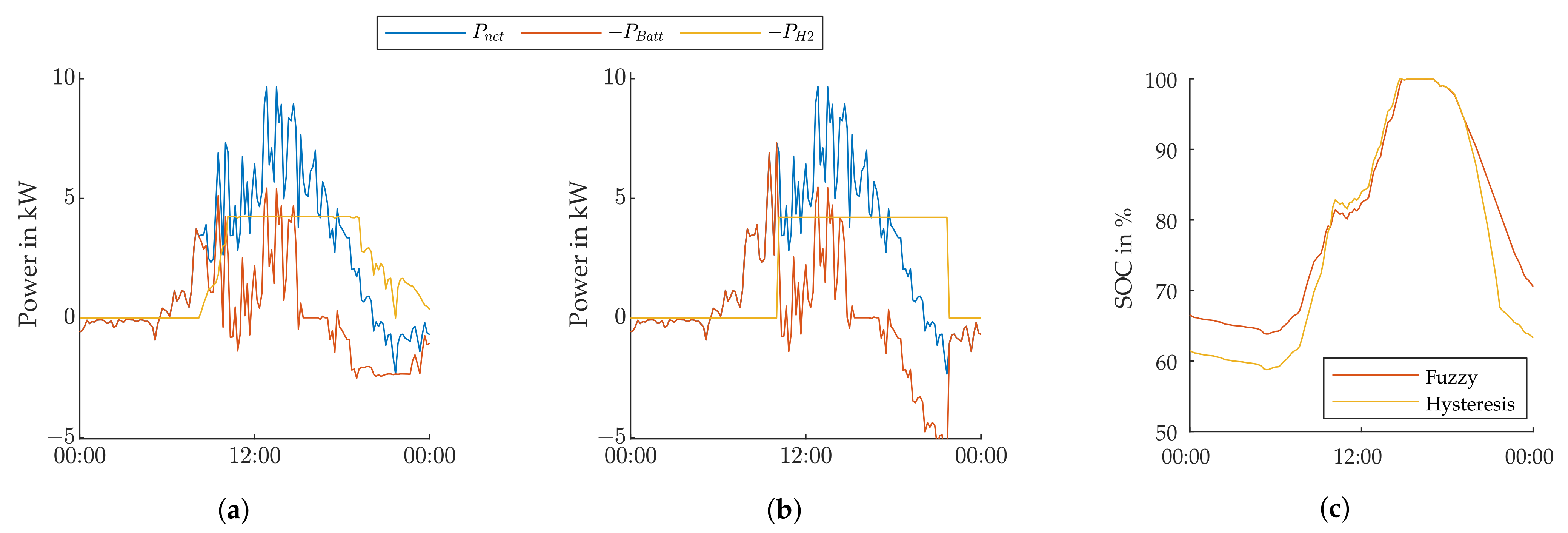
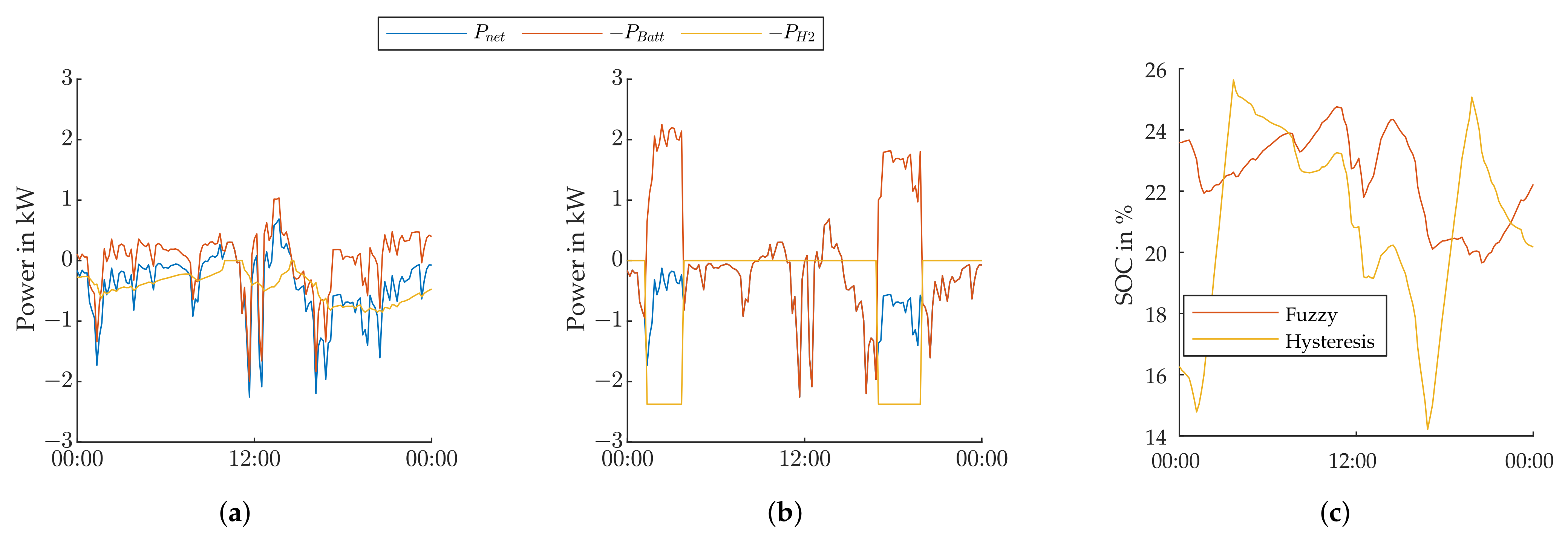
The expert tuned controller was simulated for a time frame of 1 year for the load data set No 17. According to [51], this profile is close to the daily standard load profile and thus, is considered a good starting point. The simulations were compared to a three-point hysteresis controller as a point of reference.
2.
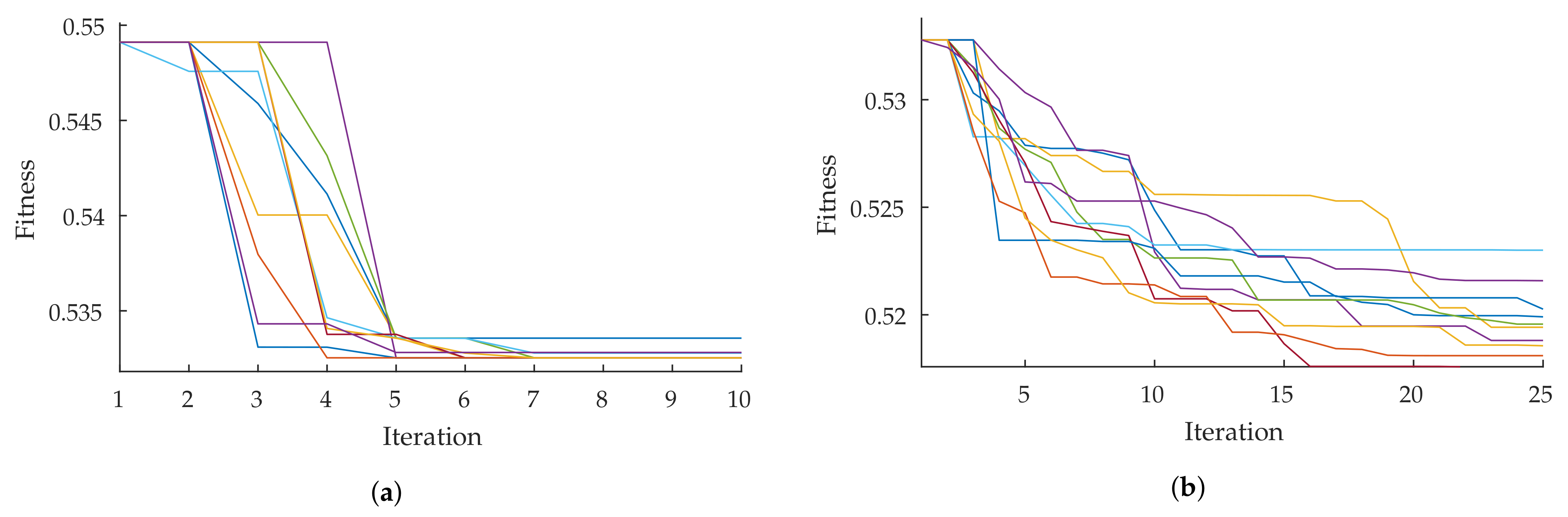
The particle swarm optimization was performed for the same load profile and compared to the expert tuned controller. The optimization followed the two-step approach described in Section 3.5.2.
3.
To test the generalizability of results, the three tunings—expert, particle swarm optimized rules, particle swarm optimized rules and membership functions—were simulated for the 65 households selected in Section 4.1. The hypothesis was that the optimized controllers performed better in terms of the indicators used in the fitness function but were less robust in terms of short-term security of supply.
4.
In the next step, the interpretability of results obtained from optimization was exploited. Expert knowledge was used to readjust the tuning of the optimized controllers aiming at retaining as much of the optimization benefits, while significantly increasing robustness.
5.
Finally, for one household, for which none of the above-mentioned controllers performed satisfactorily, further adjustments and their implications are discussed.
To discuss the simulation results, a number of performance indicators were defined. By and large, these indicators correspond to the terms used in Equation (13). However, instead of reporting the overall system losses, an indicator E S u r was constructed that illustrated how much additional electricity could be produced with the surplus H2 in the tank m H 2 , e n d m H 2 , i n i normalized by the annual load demand E l o a d , a (Equation (14)). Furthermore, the equivalent number of full battery cycles N B a t , c y c —the overall energy charged by the battery over a year divided by its nominal capacity—were reported to indicate battery usage.
E S u r = ( m H 2 , e n d m H 2 , i n i · δ H 2 · η D · η F C ) E l o a d , a · 100 %

5.1. Expert Tuned Controller

The expert tuned controller described in Section 3 was tested with load data set No 17 and the simulation framework in Section 4. To ease understanding of the behavior of the fuzzy logic energy management, the results were compared to a simple three-point hysteresis energy management approach as discussed in [54]. The SOC thresholds for switching the electrolyzer and fuel cell on and off corresponded to the values that defined the fuzzy sets of the battery SOC (see Section 3.3). Following this procedure provided a certain degree of comparability.
Figure 11 depicts the simulation results for a summer day. Given the average energy surplus, the electrolyzer should be operated. This was the case for both approaches. In contrast to the three-point hysteresis controller (Figure 11b), the fuzzy logic energy management (Figure 11a) increased the electrolyzer power gradually roughly following P n e t . Hence, the higher efficiencies of the H2-components in partial load were exploited and, by better adjusting the set points to the available net power, the more efficient power path 3, instead of paths 4 and 5, were used (compare Section 2.2).
Similarly, on a winter day (Figure 12) with an overall energy deficit, the fuel cell needed to supply the lacking energy. Whereas the fuel cell, operated by the fuzzy logic energy management system, tracked the load keeping the battery SOC relatively stable, the three-point hysteresis controller operated the fuel cell at nominal power, which in this case was considerably larger than the load. The differences between load and fuel cell power were compensated by the battery, leading to considerable fluctuations in the battery SOC.
The above-mentioned qualitative differences between the two control approaches were supported by the indicators shown in Table 3. The fuzzy logic energy management achieved a considerably higher energy surplus of 6.83% compared to 2.41% indicating a higher system efficiency. The number of fuel cell starts was slightly lower, whereas the number of electrolyzer starts was higher, suggesting that there was no straightforward connection between these indicators and the type of energy management. As expected from above discussion, the fuzzy logic energy management operated the H2-components for longer times, albeit at lower powers. The increased use of the battery by the three-point hysteresis controller was shown by the higher equivalent number of full battery cycles.
Figure 13 illustrates the distribution of losses among the different components. The three-point hysteresis control resulted in considerably higher fuel cell losses and slightly higher battery losses. The electrolyzer losses were comparable. The fuzzy logic energy management system operated the electrolyzer more efficiently, but produced more H2, leading to additional losses.
All in all, above simulations indicated that the expert tuned fuzzy logic energy management performed as expected and that it showed beneficial characteristic compared to the simpler three-point hysteresis controller.

5.2. Fuzzy Logic Energy Management System Optimization

In the next step, the expert tuned fuzzy logic energy management was optimized with the procedure described in Section 3.5. First, the rules were optimized. In order to account for the effects of random initialization, the optimization was repeated 10 times. The convergence behavior for the different runs is depicted in Figure 14a. Whereas there was a clear convergence, not all runs resulted in the same ruleset. The rule base with the best fitness was achieved in 5 out of the 10 runs and improved the fitness by 3% compared to the expert tuned controller. This tuning will be labelled OptRule.
The changes to the rule base are depicted in Table 4. The changes in rules 11 and 12 resulted in the electrolyzer being operated as soon as the battery reached a high SOC independent of P ˜ n e t . However, rule 14 was changed from NB to N, meaning that the fuel cell was only operated at nominal once P ˜ n e t was PB (rule 15). Operating the electrolyzer even though P ˜ n e t was negative could be advantageous if such a control action reduced the chances of curtailing PV power. The change in rule 4 resulted in the fuel cell being operated at low power, even if there was a certain surplus of PV power. This could be reasonable if the surplus was not large enough to get the SOC of the battery back to an acceptable region. Furthermore, it reduced the chances of having to switch on the fuel cell repeatedly if P ˜ n e t fluctuated around 0. The change in rule 1 did not seem reasonable from an expert point of view, as the fuel cell power should be increased with a decrease in P ˜ n e t and not the opposite as suggested by the optimization. A closer inspection of the data and simulations with and without a change in rule 1, showed that this change could be traced back to an idiosyncrasy of the data set. The fitness with a changed rule 1 was indeed slightly better than without (0.5325 vs. 0.5328). However, this difference resulted from a single additional fuel cell startup (124 vs. 125). Furthermore, the maximum load peak in dataset No 17 was with 5.6 kW relatively low compared to the 14.5 kW, which was used to normalize P n e t , meaning that rule 1 was close to never used and thus, did not influence the simulation results. Based on this review only the changes in rules 4, 11, 12, 14 were carried over to the optimization of the membership functions. This expert adapted tuning will be labelled OptRuleE.
The convergence behavior of the membership function optimization is shown in Figure 14b. The best out of the 10 runs resulted in a 5.7% improvement of overall fitness compared to the controller with optimized rules. The optimized membership functions are depicted in Figure 15. This tuning will be labelled OptMF. The relatively minor changes in the membership functions confirmed the assumption that the membership function optimization corresponded to a fine-tuning of the controller. The transition area between low SOC and good SOC was both widened and shifted to lower SOC levels, while the membership functions P ˜ n e t NB and N, which described a power deficit, were not changed. All other things being equal, this resulted in the battery being allowed to operate at lower SOCs and the fuel cell providing less energy at lower power levels. As long as security of supply was achieved, this led to reduced losses and less operational strain on the fuel cell. However, the latter effect was partially compensated by the shift in the membership function P ˜ H 2 P towards higher power values. On the other hand, the transition area between good and high SOC became more narrow, while P ˜ n e t P, i.e., medium power surplus, was changed towards lower values and P ˜ H 2 N towards bigger negative values. All these changes contributed towards the electrolyzer being operated more often and at higher power levels, which reduced losses from PV curtailment.
The combined changes in rule base and membership function could be visualized with the output surface of the fuzzy logic energy management (Figure 16). The increase in the blue area signified that the electrolyzer was operated more often and even if P ˜ n e t was negative. It can clearly be seen that the decision about electrolyzer operation depended solely on the battery SOC, while the level of operation depended on P ˜ n e t . The decrease in the yellow area meant that the fuel cell was operated less often at its maximum. Nevertheless, it provided low levels of support in cases of low SOC, even if P ˜ n e t was slightly positive.
The performance indicators for the different tunings—expert tuned (Expert), optimized rule base (OptRule), expert adapted optimized rule base (OptRuleE) and optimized rule and membership functions (OptMF)—are shown in Table 5.
The optimization of the rule base led primarily to decreased numbers of startups for both fuel cell and electrolyzer, while the optimization of the membership functions additionally resulted in a considerably higher energy surplus, which came as expected with decreased cycling of the battery. Furthermore, the number of fuel cell startups was reduced by more than a quarter. However, this came at the cost of increased operation time.

5.3. Fuzzy Logic Energy Management System Validation

The performance results from Section 5.2 were of limited value. While they illustrated where improvements could be located, they did not guarantee that these improvements were achieved on anything other than the training data. To verify the generalizability of the presented fuzzy logic energy management, all the controller tunings from Section 5.2 were used for simulations with the load data for the 65 households selected in Section 4.1.
The annual energy surplus in Figure 17a indicated that the optimization (OptMF) increased long-term security of supply by increasing energy surplus. Whereas there was one simulation with the expert tuned control (Expert), where this criterion was not met, it was met for all optimized cases. Figure 17b is of particular importance. In terms of short-term security of supply, it would be desirable to achieve 0 min with battery SOCs below 5%. This was achieved in 43 cases for the expert tuned controller but only in 13 cases for the optimized controller (OptMF) suggesting that the optimized controller was considerably less robust. Another interesting observation was that the expert adjustment (OptRuleE) of the rule optimization (OptRule) described in Section 5.2 restored the level of security of supply emphasizing the importance of being able to interpret optimization outcomes.
Following a similar line of argument, the thresholds that marked the transition from a low SOC to a good SOC were changed back to the expert tuned values. The result for this tuning is shown with the label OptMFE. With this relatively straightforward adjustment the level of robustness became comparable to that of the expert tuned controller, while largely retaining the improvements achieved by the optimization. This finding certainly underlines the benefit of combining an expert with an optimization-based approach.

5.4. Handles to Increase Robustness

As argued in Section 2.2, it is the objective of the energy management to always achieve security of supply. Hence, based on the validation results, the critical reader may conclude that the fuzzy logic energy management presented here was not adequate for the application at hand.
Therefore, a few handles will be discussed which allowed increasing robustness. To this end, the household with most violations of the short-term security of supply criterion was chosen as a worst-case scenario. This was household No 44. With the controller OptMFE the criterion was violated during 56.5 hours in total. Two updates to the membership functions were necessary to achieve both long-term and short-term security of supply:
1.
Increasing the thresholds that marked the transition from a low battery SOC to a good battery SOC from 0.15 and 0.25 to 0.33 and 0.34, respectively.
2.
Increasing the threshold marking the transition between P ˜ n e t is Z and P ˜ n e t is N from −0.16 to −0.08.
The first change increased the battery’s lower SOC threshold. As a result, a larger energy buffer was available for sudden and large demand peaks. The second change resulted in the fuel cell changing more rapidly to higher output power once the power deficit increased. Whereas these adjustments were indispensable to make the energy management viable for households similar to household No 44, using the same changes on other households as a measure to increase robustness came at a cost. To illustrate this matter the changed controller (labelled OptMFER) was used with household No 17 and performance indicators compared to the other reference cases (see Table 6).
The controller with increased robustness (OptMFER) had a considerably lower, but still acceptable, energy surplus at the end of the simulation year. The decreased energy surplus could be traced back to the increased activity of the fuel cell, which both started up more often and operated during longer times, leading to larger losses. The electrolyzer was also used slightly more. Whereas the performance of the controller OptMFE and OptMFER was largely comparable during summer, in spring and autumn, the increased lower battery SOC thresholds led more often to situations, where the fuel cell was operated during the night (battery SOC was below lower thresholds) and the electrolyzer was started up in the late afternoon because the battery SOC reached the upper thresholds. Such a behavior was not desirable, as the long-term storage path was used to balance short-term energy mismatch, which should be handled by the battery.
All in all, it can be stated that, even though all the load data belonged to households, the consumption patterns were so diverse that a generic controller design was either overly conservative or not sufficiently robust.

6. Conclusions and Outlook

The work presented in this article has shown the benefits of combining an expert-based with an optimization-based approach to the design of the energy management for autonomous PV hybrid systems with battery and H2 storage path. While the optimization approach is well suited to detect areas of improvement, the optimization results need to be evaluated in a broader context and if necessary, adjusted to avoid over-fitting to specific training data. To ease this process, the optimization with a particle swarm was adjusted in order to maintain interpretability of the control tuning. Following this procedure, an improved energy management based on fuzzy logic control was developed and validated. Furthermore, it was demonstrated that the most common practice of validating an energy management system based on a single data set is of very limited validity, as consumption patterns are rather diverse posing different requirements to the control system. The diversity can be met by a conservative tuning. However, this comes at a cost both in terms of efficiency and component stress. The trade-off between generalizability and performance could be eased in the future by creating classes of load profiles and developing an apt controller tuning for each class.
Additional future research directions include more detailed component modelling, prediction algorithms for load and generation, a closer scrutiny of the impact of the fuzzy logic controller’s internal methods and the parameters used by the particle swarm optimization as well as the integration and combined or iterative optimization of component sizing and energy management. In the following some comments on these areas and their relationship with this article are given.
The simulation framework in this study was designed to allow sufficiently fast simulations, which was a prerequisite both for optimization and subsequent validation. Therefore, relatively simple look-up tables were used. In future work, the impact of model granularity on performance and robustness is to be examined in more detail. Moreover, advanced component models should be introduced to represent degradation and ageing effects.
Short-term predictions combined with a model-based control approach would allow the implementation of improved anticipatory control actions, while long-term predictions could be used to realize adjustable battery SOC thresholds. Both measures are likely to be beneficial in terms of overall system efficiency and security of supply.
This study used the most common configuration of a fuzzy logic controller and particle swarm optimization. While these provided a good starting point and allowed continuity with prior work in the field, the impact of these design choices and possible alternatives for the application in off-grid systems with hybrid storage should be further scrutinized. In the case of the fuzzy logic controller, these are in particular different shapes of membership functions and methods for aggregation. For the particle swarm optimization, the number of particles and iterations should be investigated more closely.
Finally, the integration and combined or iterative optimization of component sizing and energy management is likely to have considerable potential. As discussed in Section 2.2, increasing system efficiency is not an aim in itself, but can lead to smaller sized components and increased security of supply. Whereas the main objective in this article was to show the impact of different controller tunings given a fixed hardware setup, in a next step this knowledge is to be used to update the sizing of components.
All in all, it was demonstrated that fuzzy logic control presents an interesting method for the energy management of autonomous systems with hybrid storage, especially if combined with an optimization approach. Improvement in the energy management allows for smaller dimensioning of all components in the system and reduces early failures due to fatigue. Considering that autonomous PV hybrid systems are typically employed in remote places and rural electrification, where low cost and high reliability are decisive, the here presented energy management system can considerably contribute to their successful application.

Author Contributions

Conceptualization, L.G. and T.B.; investigation, L.G.; software, L.G.; supervision, T.B.; visualization, L.G.; writing—original draft, L.G.; writing—review and editing, T.B. All authors have read and agreed to the published version of the manuscript.

Funding

Open access funding by the publication fund of the TU Dresden.

Institutional Review Board Statement

Not applicable.

Informed Consent Statement

Not applicable.

Data Availability Statement

Not applicable.

Conflicts of Interest

The authors declare no conflict of interest.

Abbreviations

The following abbreviations are used in this manuscript:
E l o a d , a  Annual energy consumption in kWh
E l o s s , a  Aggregated annual energy losses in kWh
E P V , a  Annual PV generation in kWh
E S u r  Relative surplus energy at the end of the year in % (compare Equation (14))
F Fitness of particle in particle swarm optimization
f i  Objective function i
g b e s t  Best global past position among all particles
H2 Hydrogen
k C O A  Centre of area
m H 2  H2 stored in tank in kg
N Negative
NB Negative big
N B a t , c y c  Equivalent number of full battery cycles
N S O C , l o w  Time battery SOC is below 5% in min
N S t a r t , E L  Number of electrolyzer starts
N S t a r t , F C  Number of fuel cell starts
P Positive
OptMF Controller tuning optimized membership functions based on OptRuleE
OptMFE Controller tuning optimized membership functions, expert adjusted
OptMFER Controller tuning based on OptMFE, adjusted for robustness
OptRule Controller tuning with optimized rule base
OptRuleE Controller tuning with optimized rule base, expert adjusted
P B a t t  Battery output power
P E L  Electrolyzer output power
P F C  Fuel cell output power
P H 2  Power of the H2 storage path (if positive equal to P F C , if negative equal to P E L )
P ˜ H 2 P H 2 , normalized
P L o a d  Load power
P n e t  Power difference between P P V and P L o a d
P ˜ n e t P n e t , normalized
P P V  PV power generation
P P V , c u r t  Curtailed PV power
PB Positive big
p b e s t ( n )  Best past position of particle n
PV Photovoltaic
q Penalty parameter
R Rule in the fuzzy rule base
SOC State of charge
T E L  Time electrolyzer is in operation in h
T F C  Time fuel cell is in operation in h
v ( n )  Velocity of particle n
x ( n )  Position of particle n
Z Zero
δ H 2  Higher heating value
η B a t t  Battery round-trip efficiency
η D  DC–DC converter efficiency
η E L  Electrolyzer average efficiency
η F C  Fuel cell average efficiency
η I N  Inverter efficiency
η P V  PV average efficiency
μ A  Membership function of fuzzy set A

References

  1. Bocklisch, T. Hybrid Energy Storage Approach for Renewable Energy Applications. J. Energy Storage 2016, 8, 311–319. [Google Scholar] [CrossRef]
  2. Kyriakarakos, G.; Dounis, A.I.; Arvanitis, K.G.; Papadakis, G. A Fuzzy Logic Energy Management System for Polygeneration Microgrids. Renew. Energy 2012, 41, 315–327. [Google Scholar] [CrossRef]
  3. Erdinc, O.; Vural, B.; Uzunoglu, M. A Wavelet-Fuzzy Logic Based Energy Management Strategy for a Fuel Cell/Battery/Ultra-Capacitor Hybrid Vehicular Power System. J. Power Sources 2009, 194, 369–380. [Google Scholar] [CrossRef]
  4. Ferreira, A.A.; Pomilio, J.A.; Spiazzi, G.; Araujo Silva, L. Energy Management Fuzzy Logic Supervisory for Electric Vehicle Power Supplies System. IEEE Trans. Power Electron. 2008, 23, 107–115. [Google Scholar] [CrossRef]
  5. Li, C.Y.; Liu, G.P. Optimal Fuzzy Power Control and Management of Fuel Cell/Battery Hybrid Vehicles. J. Power Sources 2009, 192, 525–533. [Google Scholar] [CrossRef]
  6. Vivas, F.J.; De las Heras, A.; Segura, F.; Andújar, J.M. A Review of Energy Management Strategies for Renewable Hybrid Energy Systems with Hydrogen Backup. Renew. Sustain. Energy Rev. 2018, 82, 126–155. [Google Scholar] [CrossRef]
  7. Stegner, C.; Glaß, O.; Beikircher, T. Comparing Smart Metered, Residential Power Demand with Standard Load Profiles. Sustain. Energy Grids Netw. 2019, 20, 100248. [Google Scholar] [CrossRef]
  8. Bocklisch, T. Intelligente Dezentrale Energiespeichersysteme. UWF UmweltWirtschaftsForum 2014, 22, 63–70. [Google Scholar] [CrossRef]
  9. Kyriakarakos, G.; Dounis, A.I.; Arvanitis, K.G.; Papadakis, G. A Fuzzy Cognitive Maps–Petri Nets Energy Management System for Autonomous Polygeneration Microgrids: Theoretical Issues and Advanced Applications on Fuzzy Cognitive Maps. Appl. Soft Comput. 2012, 12, 3785–3797. [Google Scholar] [CrossRef]
  10. Bilodeau, A.; Agbossou, K. Control Analysis of Renewable Energy System with Hydrogen Storage for Residential Applications. J. Power Sources 2006, 162, 757–764. [Google Scholar] [CrossRef]
  11. Calderón, A.J.; González, I.; Calderón, M. Management of a PEM Electrolyzer in Hybrid Renewable Energy Systems. In Fuzzy Modeling and Control: Theory and Applications; Matía, F., Marichal, G.N., Jiménez, E., Eds.; Atlantis Computational Intelligence Systems; Atlantis Press: Paris, France, 2014; Volume 9, pp. 217–233. [Google Scholar]
  12. Safari, S.; Ardehali, M.M.; Sirizi, M.J. Particle Swarm Optimization Based Fuzzy Logic Controller for Autonomous Green Power Energy System with Hydrogen Storage. Energy Convers. Manag. 2013, 65, 41–49. [Google Scholar] [CrossRef]
  13. García, P.; Torreglosa, J.P.; Fernández, L.M.; Jurado, F. Optimal Energy Management System for Stand-Alone Wind Turbine/Photovoltaic/Hydrogen/Battery Hybrid System with Supervisory Control Based on Fuzzy Logic. Int. J. Hydrogen Energy 2013, 38, 14146–14158. [Google Scholar] [CrossRef]
  14. Erdinc, O.; Uzunoglu, M. The Importance of Detailed Data Utilization on the Performance Evaluation of a Grid-Independent Hybrid Renewable Energy System. Int. J. Hydrogen Energy 2011, 36, 12664–12677. [Google Scholar] [CrossRef]
  15. Sarvi, M.; Avanaki, I.N. An Optimized Fuzzy Logic Controller by Water Cycle Algorithm for Power Management of Stand-Alone Hybrid Green Power Generation. Energy Convers. Manag. 2015, 106, 118–126. [Google Scholar] [CrossRef]
  16. Boukettaya, G.; Krichen, L.; Ouali, A. Fuzzy Logic Supervisor for Power Control of an Isolated Hybrid Energy Production Unit. Int. J. Electr. Power Eng. 2007, 1, 279–285. [Google Scholar]
  17. Habib, M.; Ladjici, A.A.; Harrag, A. Microgrid Management Using Hybrid Inverter Fuzzy-Based Control. Neural Comput. Appl. 2019, 32, 1–19. [Google Scholar] [CrossRef]
  18. Ganguly, P.; Kalam, A.; Zayegh, A. Fuzzy Logic-Based Energy Management System of Stand-Alone Renewable Energy System for a Remote Area Power System. Aust. J. Electr. Electron. Eng. 2019, 16, 21–32. [Google Scholar] [CrossRef]
  19. Berrazouane, S.; Mohammedi, K. Parameter Optimization via Cuckoo Optimization Algorithm of Fuzzy Controller for Energy Management of a Hybrid Power System. Energy Convers. Manag. 2014, 78, 652–660. [Google Scholar] [CrossRef]
  20. Thameem Ansari, M.; Velusami, S. Dual Mode Linguistic Hedge Fuzzy Logic Controller for an Isolated Wind–Diesel Hybrid Power System with Superconducting Magnetic Energy Storage Unit. Energy Convers. Manag. 2010, 51, 169–181. [Google Scholar] [CrossRef]
  21. Al-Sakkaf, S.; Kassas, M.; Khalid, M.; Abido, M.A. An Energy Management System for Residential Autonomous DC Microgrid Using Optimized Fuzzy Logic Controller Considering Economic Dispatch. Energies 2019, 12, 1457. [Google Scholar] [CrossRef] [Green Version]
  22. Weyers, C.; Bocklisch, T. Simulation-Based Investigation of Energy Management Concepts for Fuel Cell – Battery – Hybrid Energy Storage Systems in Mobile Applications. Energy Procedia 2018, 155, 295–308. [Google Scholar] [CrossRef]
  23. Arcos-Aviles, D.; García-Gutièrrez, G.; Guinjoan, F.; Carrera, E.V.; Pascual, J.; Ayala, P.; Marroyo, L.; Motoasca, E. Adjustment of the Fuzzy Logic Controller Parameters of the Energy Management Strategy of a Grid-Tied Domestic Electro-Thermal Microgrid Using the Cuckoo Search Algorithm. In Proceedings of the IECON 2019—45th Annual Conference of the IEEE Industrial Electronics Society, Lisbon, Portugal, 14–17 October 2019; Volume 1, pp. 279–285. [Google Scholar] [CrossRef]
  24. Arcos-Aviles, D.; Pacheco, D.; Pereira, D.; Garcia-Gutierrez, G.; Carrera, E.V.; Ibarra, A.; Ayala, P.; Martínez, W.; Guinjoan, F. A Comparison of Fuzzy-Based Energy Management Systems Adjusted by Nature-Inspired Algorithms. Appl. Sci. 2021, 11, 1663. [Google Scholar] [CrossRef]
  25. Athari, M.H.; Ardehali, M.M. Operational Performance of Energy Storage as Function of Electricity Prices for On-Grid Hybrid Renewable Energy System by Optimized Fuzzy Logic Controller. Renew. Energy 2016, 85, 890–902. [Google Scholar] [CrossRef]
  26. Vivas, F.J.; Segura, F.; Andújar, J.M.; Palacio, A.; Saenz, J.L.; Isorna, F.; López, E. Multi-Objective Fuzzy Logic-Based Energy Management System for Microgrids with Battery and Hydrogen Energy Storage System. Electronics 2020, 9, 1074. [Google Scholar] [CrossRef]
  27. Faisal, M.; Hannan, M.A.; Ker, P.J.; Rahman, M.S.A.; Begum, R.A.; Mahlia, T.M.I. Particle Swarm Optimised Fuzzy Controller for Charging–Discharging and Scheduling of Battery Energy Storage System in MG Applications. Energy Rep. 2020, 6, 215–228. [Google Scholar] [CrossRef]
  28. Babu, T.S.; Vasudevan, K.R.; Ramachandaramurthy, V.K.; Sani, S.B.; Chemud, S.; Lajim, R.M. A Comprehensive Review of Hybrid Energy Storage Systems: Converter Topologies, Control Strategies and Future Prospects. IEEE Access 2020, 8, 148702–148721. [Google Scholar] [CrossRef]
  29. Welch, R.; Venayagamoorthy, G.K. A Fuzzy-PSO Based Controller for a Grid Independent Photovoltaic System. In Proceedings of the IEEE Swarm Intelligence Symposium, Honolulu, HI, USA, 1–5 April 2007. [Google Scholar] [CrossRef] [Green Version]
  30. Meng, L.; Sanseverino, E.R.; Luna, A.; Dragicevic, T.; Vasquez, J.C.; Guerrero, J.M. Microgrid Supervisory Controllers and Energy Management Systems: A Literature Review. Renew. Sustain. Energy Rev. 2016, 60, 1263–1273. [Google Scholar] [CrossRef]
  31. Paulitschke, M.; Bocklisch, T.; Böttiger, M. Sizing Algorithm for a PV-Battery-H2-Hybrid System Employing Particle Swarm Optimization. Energy Procedia 2015, 73, 154–162. [Google Scholar] [CrossRef] [Green Version]
  32. Paulitschke, M.; Bocklisch, T.; Böttiger, M. Comparison of Particle Swarm and Genetic Algorithm Based Design Algorithms for PV-Hybrid Systems with Battery and Hydrogen Storage Path. Energy Procedia 2017, 135, 452–463. [Google Scholar] [CrossRef]
  33. Saxena, S.; Hendricks, C.; Pecht, M. Cycle Life Testing and Modeling of Graphite/LiCoO2 Cells under Different State of Charge Ranges. J. Power Sources 2016, 327, 394–400. [Google Scholar] [CrossRef]
  34. Bocklisch, T. Optimierendes Energiemanagement von Brennstoffzelle-Direktspeicher-Hybridsystemen. Ph.D. Thesis, Technische Universität Chemnitz, Chemnitz, Germany, 2009. [Google Scholar]
  35. Barbir, F. PEM Electrolysis for Production of Hydrogen from Renewable Energy Sources. Solar Hydrog. 2005, 78, 661–669. [Google Scholar] [CrossRef]
  36. Pham, T.T.C. Introduction to Fuzzy Sets, Fuzzy Logic, and Fuzzy Control Systems; CRC Press: Boca Raton, FL, USA, 2001. [Google Scholar]
  37. Mamdani, E.H.; Assilian, S. An Experiment in Linguistic Synthesis with a Fuzzy Logic Controller. Int. J. Man-Mach. Stud. 1975, 7, 1–13. [Google Scholar] [CrossRef]
  38. Zadeh, L.A. Fuzzy Sets. Inf. Control 1965, 8, 338–353. [Google Scholar] [CrossRef] [Green Version]
  39. Schulz, G.; Graf, C. Regelungstechnik 2: Mehrgrößenregelung, Digitale Regelungstechnik, Fuzzy-Regelung, 3rd ed.; De Gruyter: München, Germany, 2013. [Google Scholar] [CrossRef]
  40. Rosyadi, M.; Muyeen, S.M.; Takahashi, R.; Tamura, J. A Design Fuzzy Logic Controller for a Permanent Magnet Wind Generator to Enhance the Dynamic Stability of Wind Farms. Appl. Sci. 2012, 2, 780–800. [Google Scholar] [CrossRef] [Green Version]
  41. Michels, K.; Kruse, R.; Klawonn, F.; Nürnberger, A. Fuzzy-Regelung: Grundlagen, Entwurf, Analyse; Springer-Lehrbuch; Springer: Berlin/Heidelberg, Germany, 2002. [Google Scholar] [CrossRef]
  42. Hussain, S.; Ahmed, M.A.; Lee, K.B.; Kim, Y.C. Fuzzy Logic Weight Based Charging Scheme for Optimal Distribution of Charging Power among Electric Vehicles in a Parking Lot. Energies 2020, 13, 3119. [Google Scholar] [CrossRef]
  43. Pedrycz, W. Why Triangular Membership Functions? Fuzzy Sets Syst. 1994, 64, 21–30. [Google Scholar] [CrossRef]
  44. Barua, A.; Mudunuri, L.; Kosheleva, O. Why Trapezoidal and Triangular Membership Functions Work So Well: Towards a Theoretical Explanation. J. Uncertain Syst. 2014, 8, 164–168. [Google Scholar]
  45. DIN. DIN 18015-3:2016-09, Electrical Installations in Residential Buildings—Part 3: Wiring and Disposition of Electrical Equipment; Technical Report; Beuth Verlag GmbH: Berlin, Germany, 2016. [Google Scholar] [CrossRef]
  46. Kennedy, J.; Eberhart, R. Particle Swarm Optimization. In Proceedings of the ICNN’95 - International Conference on Neural Networks, Perth, Australia, 27 November–1 December 1995; Volume 4, pp. 1942–1948. [Google Scholar] [CrossRef]
  47. Eberhart, R.; Kennedy, J. A New Optimizer Using Particle Swarm Theory. In Proceedings of the MHS’95— Sixth International Symposium on Micro Machine and Human Science, Nagoya, Japan, 4–6 October 1995; pp. 39–43. [Google Scholar] [CrossRef]
  48. Kennedy, J.F.; Eberhart, R.C.; Shi, Y. Swarm Intelligence; The Morgan Kaufmann Series in Evolutionary Computation; Morgan Kaufmann Publishers: San Francisco, CA, USA, 2001. [Google Scholar]
  49. Piotrowski, A.P.; Napiorkowski, J.J.; Piotrowska, A.E. Population Size in Particle Swarm Optimization. Swarm Evol. Comput. 2020, 58, 100718. [Google Scholar] [CrossRef]
  50. Arora, J.S. Introduction to Optimum Design, 3rd ed.; Academic Press: Boston, MA, USA, 2011. [Google Scholar]
  51. Tjaden, T.; Bergner, J.; Weniger, J.; Quaschning, V. Representative Electrical Load Profiles of Residential Buildings in Germany with a Temporal Resolution of One Second; ResearchGate: Berlin, Germany, 2015. [Google Scholar] [CrossRef]
  52. Böttiger, M.; Paulitschke, M.; Bocklisch, T. Systematic Experimental Pulse Test Investigation for Parameter Identification of an Equivalent Based Lithium-Ion Battery Model. Energy Procedia 2017, 135, 337–346. [Google Scholar] [CrossRef]
  53. Bocklisch, T.; Böttiger, M.; Paulitschke, M. Multi-Storage Hybrid System Approach and Experimental Investigations. Energy Procedia 2014, 46, 186–193. [Google Scholar] [CrossRef] [Green Version]
  54. Zhou, K.; Ferreira, J.A.; Haan, S. Optimal Energy Management Strategy and System Sizing Method for Stand-Alone Photovoltaic-Hydrogen Systems. Int. J. Hydrogen Energy 2008, 33, 477–489. [Google Scholar] [CrossRef]
Figure 1. Topology of autonomous PV hybrid system with battery and H2 storage path.
Energies 14 01777 g001
Figure 2. Block diagram of a fuzzy logic controller.
Energies 14 01777 g002
Figure 3. Membership functions. (a) Input 1: battery state of charge (SOC). (b) Input 2: net power P ˜ n e t . (c) Output: electrolyzer/fuel cell power P ˜ H 2 .
Energies 14 01777 g003
Figure 4. Block diagram of fuzzy logic controller tuning based on particle swarm optimization.
Energies 14 01777 g004
Figure 5. Flowchart of fuzzy logic controller tuning based on particle swarm optimization.
Energies 14 01777 g005
Figure 6. Data input to simulation framework. (a) PV data. (b) Load data household No 17.
Energies 14 01777 g006
Figure 7. (a) Monthly averages in power consumption. (b) Maximum power by household (15 min average).
Energies 14 01777 g007
Figure 8. (a) Load duration curve based on daily averages. (b) Zoomed version of (a).
Energies 14 01777 g008
Figure 9. (a) Load duration curve based on 10-min averages. (b) Zoomed version of (a).
Energies 14 01777 g009
Figure 10. Component models including converter losses. (a) Battery: ΔSOC look-up table. (b) Electrolyzer: ΔH2 look-up table. (c) Fuel cell: ΔH2 look-up table.
Energies 14 01777 g010
Figure 11. Timeseries summer day. (a) Expert tuned fuzzy logic controller. (b) Three-point hysteresis controller. (c) Battery SOC profiles.
Energies 14 01777 g011
Figure 12. Timeseries winter day. (a) Expert tuned fuzzy logic controller. (b) Three-point hysteresis controller. (c) Battery SOC profiles.
Energies 14 01777 g012
Figure 13. Distribution of losses.
Energies 14 01777 g013
Figure 14. Convergence behavior of particle swarm optimization. (a) Rule base optimization. (b) Membership function optimization.
Energies 14 01777 g014
Figure 15. Membership functions: expert tuned (ac) and optimized (df). (a,d) Input 1: battery SOC. (b,e) Input 2: Net Power P ˜ n e t . (c,f) Output: electrolyzer/fuel cell power P ˜ H 2 .
Energies 14 01777 g015
Figure 16. Fuzzy logic energy management output surface. (a) Expert tuned. (b) Optimized.
Energies 14 01777 g016
Figure 17. Performance indicators for several controller tunings. (a) Annual energy surplus; (b) time with low battery SOC; (c) number of electrolyzer starts; (d) electrolyzer operation time; (e) number of fuel cell starts; (e) fuel cell operation time; (f) fuel cell operation time; (g) equivalent number of full battery cycles.
Energies 14 01777 g017
Table 1. Fuzzy logic controller rule base.
1.If (SOC is low)and ( P ˜ n e t is NB)then ( P ˜ H 2 is PB)
2.If (SOC is low)and ( P ˜ n e t is N)then ( P ˜ H 2 is PB)
3.If (SOC is low)and ( P ˜ n e t is Z)then ( P ˜ H 2 is P)
4.If (SOC is low)and ( P ˜ n e t is P)then ( P ˜ H 2 is Z)
5.If (SOC is low)and ( P ˜ n e t is PB)then ( P ˜ H 2 is Z)
6.If (SOC is good)and ( P ˜ n e t is NB)then ( P ˜ H 2 is Z)
7.If (SOC is good)and ( P ˜ n e t is N)then ( P ˜ H 2 is Z)
8.If (SOC is good)and ( P ˜ n e t is Z)then ( P ˜ H 2 is Z)
9.If (SOC is good)and ( P ˜ n e t is P)then ( P ˜ H 2 is Z)
10.If (SOC is good)and ( P ˜ n e t is PB)then ( P ˜ H 2 is Z)
11.If (SOC is high)and ( P ˜ n e t is NB)then ( P ˜ H 2 is Z)
12.If (SOC is high)and ( P ˜ n e t is N)then ( P ˜ H 2 is Z)
13.If (SOC is high)and ( P ˜ n e t is Z)then ( P ˜ H 2 is N)
14.If (SOC is high)and ( P ˜ n e t is P)then ( P ˜ H 2 is NB)
15.If (SOC is high)and ( P ˜ n e t is PB)then ( P ˜ H 2 is NB)
Table 2. H2 model parameters.
P Nom η ( δ H 2 ) P Peri , const P Peri , var
Electrolyzer4 kW70%20%80%
Fuel cell2.5 kW40%20%80%
Table 3. Comparison between expert tuned controller and three-point hysteresis controller.
E Sur
in %
N Start , FC T FC
in h
N Start , EL T EL
in h
T SOC , low
in min
N Bat , cyc
Fuzzy6.83155173426120460101
Hysteresis2.4116850719412580123
Table 4. Optimized fuzzy logic controller rule base.
1.If (SOC is low)and ( P ˜ n e t is NB)then ( P ˜ H 2 is PB)→ P
2.If (SOC is low)and ( P ˜ n e t is N)then ( P ˜ H 2 is PB)
3.If (SOC is low)and ( P ˜ n e t is Z)then ( P ˜ H 2 is P)
4.If (SOC is low)and ( P ˜ n e t is P)then ( P ˜ H 2 is Z)→ P
5.If (SOC is low)and ( P ˜ n e t is PB)then ( P ˜ H 2 is Z)
6.If (SOC is good)and ( P ˜ n e t is NB)then ( P ˜ H 2 is Z)
7.If (SOC is good)and ( P ˜ n e t is N)then ( P ˜ H 2 is Z)
8.If (SOC is good)and ( P ˜ n e t is Z)then ( P ˜ H 2 is Z)
9.If (SOC is good)and ( P ˜ n e t is P)then ( P ˜ H 2 is Z)
10.If (SOC is good)and ( P ˜ n e t is PB)then ( P ˜ H 2 is Z)
11.If (SOC is high)and ( P ˜ n e t is NB)then ( P ˜ H 2 is Z)→ N
12.If (SOC is high)and ( P ˜ n e t is N)then ( P ˜ H 2 is Z)→ N
13.If (SOC is high)and ( P ˜ n e t is Z)then ( P ˜ H 2 is N)
14.If (SOC is high)and ( P ˜ n e t is P)then ( P ˜ H 2 is NB)→ N
15.If (SOC is high)and ( P ˜ n e t is PB)then ( P ˜ H 2 is NB)
Table 5. Result of optimization run.
E Sur
in %
N Start , FC T FC
in h
N Start , EL T EL
in h
T SOC , low
in min
N Bat , cyc
Expert6.83155173426120460101
OptRule6.88124173721921030101
OptRuleE6.88125173621921030100
OptMF7.279018392181904097
Table 6. Results of simulation runs for household No 17.
E Sur
in %
N Start , FC T FC
in h
N Start , EL T EL
in h
T SOC , low
in min
N Bat , cyc
Expert6.83155173426120460101
OptMF7.279018392181904097
OptMFE7.0511617772201912097
OptMFER5.8814420172281965096
Publisher’s Note: MDPI stays neutral with regard to jurisdictional claims in published maps and institutional affiliations.

