Article

Innovative Application of Model-Based Predictive Control for Low-Voltage Power Distribution Grids with Significant Distributed Generation †

1
PROMES-CNRS (UPR 8521), Université de Perpignan Via Domitia, Rambla de la Thermodynamique, Tecnosud, 66100 Perpignan, France
2
Instituto de Ciencias de la Ingeniería, Universidad de O’Higgins, O’Higgins 2841935, Chile
*
Author to whom correspondence should be addressed.
This paper is an extended version of the paper entitled A model-based predictive control for power distribution grids with prolific distributed generation: A case study, published in the proceedings of the 2020 IEEE International Conference on Environment and Electrical Engineering and 2020 IEEE Industrial and Commercial Power Systems Europe (EEEIC / I&CPS Europe), Madrid, Spain, 2020; pp. 1–6.
Energies 2021, 14(6), 1773; https://doi.org/10.3390/en14061773
Submission received: 25 January 2021 / Revised: 26 February 2021 / Accepted: 17 March 2021 / Published: 23 March 2021

Abstract

:
In past decades, the deployment of renewable-energy-based power generators, namely solar photovoltaic (PV) power generators, has been projected to cause a number of new difficulties in planning, monitoring, and control of power distribution grids. In this paper, a control scheme for flexible asset management is proposed with the aim of closing the gap between power supply and demand in a suburban low-voltage power distribution grid with significant penetration of solar PV power generation while respecting the different systems’ operational constraints, in addition to the voltage constraints prescribed by the French distribution grid operator (ENEDIS). The premise of the proposed strategy is the use of a model-based predictive control (MPC) scheme. The flexible assets used in the case study are a biogas plant and a water tower. The mixed-integer nonlinear programming (MINLP) setting due to the water tower ON/OFF controller greatly increases the computational complexity of the optimisation problem. Thus, one of the contributions of the paper is a new formulation that solves the MINLP problem as a smooth continuous one without having recourse to relaxation. To determine the most adequate size for the proposed scheme’s sliding window, a sensitivity analysis is carried out. Then, results given by the scheme using the previously determined window size are analysed and compared to two reference strategies based on a relaxed problem formulation: a single optimisation yielding a weekly operation planning and a MPC scheme. The proposed problem formulation proves effective in terms of performance and maintenance of acceptable computational complexity. For the chosen sliding window, the control scheme drives the power supply/demand gap down from the initial one up to 38%.

1. Introduction

In recent years, the growing penetration of distributed generation (DG) into power distribution grids has been having a deep impact on these grids [1]. The deployment of distributed generators results in bidirectional power flow [2] and is projected to worsen voltage fluctuations and increase the risk of power backflow from low-voltage power distribution grids to medium-voltage ones. This is mainly due to wind and solar, which are intermittent energy sources depending on geographical locations and weather conditions [3].
Power distribution grid operators are contractually required to provide safe and reliable service to their customers and, as a result, are complying with several regulations, mainly on voltage constraints, voltage drop gradients, and current levels [4]. However, deployment of distributed generators is expected to make compliance with such constraints increasingly difficult. In addition, it triggers plenty of safety and quality issues, including short-circuits, power outages, and equipment damage [5,6]. The penetration of distributed generation into power distribution grids is also behind planning, legal, and regulatory issues [7].
The smart grid paradigm was conceived to tackle monitoring and control problems in power distribution grids [2]. Its building blocks include boosting grid observability through forecasting of grid load [8] and distributed generation [9], deployment of an advanced metering infrastructure (for instance, through the smart meter Linky in France), and smart management schemes which aim to balance out power supply and demand. Optimal power flow [10,11,12,13,14,15], demand-side management [16,17,18,19,20,21], and multi-agent systems [22,23,24,25,26] are some of the most abundant techniques in the scientific literature. Depending on the application, which can range from dimensioning and planning of power grid infrastructure to real-time monitoring and control, and the technical and computational constraints, one technique may be more appropriate than another. For instance, the voltage levels in the power distribution grid at hand determine which of these techniques is the best suited when it comes to developing a control scheme. A survey of smart management tools for power distribution grids with prolific distributed generation is provided by the present paper’s authors in [27].
Modern power distribution grids group several distributed generators and storage devices. Therefore, it stands to reason to use these generators and storage devices to balance power supply and demand. The problem to solve can then be formulated as a minimisation one, where the aim is to minimise the cumulated difference between power supply and demand over a time horizon. The proposed strategy combines flexible asset management approach [28,29,30] and implicit model-based predictive control (MPC) [31,32,33,34]. Because power distribution grids are subject to intermittent renewable-energy-based power generation as well as stochastic electricity demand, the suitability of MPC to the monitoring and control of these power grids is plain. Such disturbances can provoke more or less serious failures and low-voltage power distribution grids, because of their weakly meshed (often radial) structure, are especially prone to cascading failures. Economic convenience edged out the extra layer of safety at the planning stage of these power grids, but, in the context of growing distributed generation, this choice has not aged well. As a consequence, anticipation of future issues that may affect the considered system is paramount [27].
In this paper, a MPC-based strategy taking advantage of distributed generators and non-electrical power storage systems owned by third parties (a biogas plant and a water tower) has been developed by PROMES-CNRS (“Processes, Materials and Solar Energy”) in order to balance power supply and demand and limit instances of voltage overflow in a low-voltage power distribution grid in southern France, while upholding the assets’ operational constraints [35,36]. The case study is a simulated one. This work falls under the ADEME (the French agency for ecological transition) “Smart Occitania” project which responds to a concrete need expressed by ENEDIS for smart management tools and computationally-tractable algorithms for rural and suburban low-voltage power distribution grids with prolific distributed generation. One of the objectives of the project is to evaluate the potential of MPC for upper-level power flow management and curtailment of voltage fluctuations in low-voltage power distribution grids. In addition, ENEDIS and PROMES-CNRS investigate in the considered case study the use of a biogas plant and a water tower owned by third parties as flexible assets in the control scheme. The biogas plant is controlled by a continuous signal. However, the operation of the water tower is subject to an ON/OFF controller and the discrete nature of the water tower’s control signal makes the problem to solve a mixed-integer nonlinear programming (MINLP) one.
MINLP problems have received a great deal of attention in the past few years with a wide range of contributions from researchers in applied mathematics on theoretical, algorithmic, and computational aspects. MINLP is a challenging research field and existing solvers able to tackle it have significant limitations [37], further worsened in the case of non-convex constraints [38]. When the problem is convex, quite effective algorithms, including heuristic algorithms, are available in the literature. However, non-convex MINLP problems, which are much more difficult to solve, arise in several areas of engineering, in particular energy resource management [39,40,41,42]. For further information on the available algorithms and software one can use to solve MINLP problems, the reader is referred to [43,44,45,46]. A survey of non-convex MINLP (optimisation tools, algorithms, etc.) is provided in [38,47]. The main difficulty in modelling the problem addressed by PROMES-CNRS as a MINLP one comes from the fact that it is both nonlinear and non-convex. This is due to the nonlinear non-convex hard constraints representing Kirchhoff’s laws, which are polynomial equality constraints (see Equation (22)). While several techniques from the literature could be implemented and tested, a relaxation of the problem, whether at the modelling stage or the resolution stage, is the usual route to bypass the difficulties related to MINLP [38,47,48]. Instead, we propose a problem formulation that allows us to bypass the MINLP framework of the optimisation problem without relaxing the ON/OFF constraint of the water tower controller. This formulation, dubbed switch control, takes the problem out of its MINLP setting and makes it a continuous nonlinear optimisation one. In fact, by optimising the instants at which the water tower’s controller switches from one state to the next, the discrete control signal is modelled as a continuous one.
The paper is organised as follows. In Section 2, the case study is presented, an overview of the proposed control strategy is given. and models of the considered low-voltage power distribution grid and the two flexible assets used in the case study are formulated. Section 3 provides an explanation of the proposed model-based predictive control strategy. Then, the MINLP problem formulation is presented and the new formulation proposed in this paper is introduced. In Section 4, a sensitivity analysis is performed in order to highlight the most adequate sliding window size. Afterwards, results given by the proposed control strategy are compared with those of two reference strategies. The first reference strategy is a weekly operation planning which provides a heuristic lower bound for the objective function final value (i.e., cumulated difference between power supply and demand). The second reference strategy is a MPC scheme based on a relaxed problem formulation. The paper ends with a conclusion and an outlook to future works (Section 5). The post-treatment algorithms are detailed in Appendix A.

2. Materials and Methods
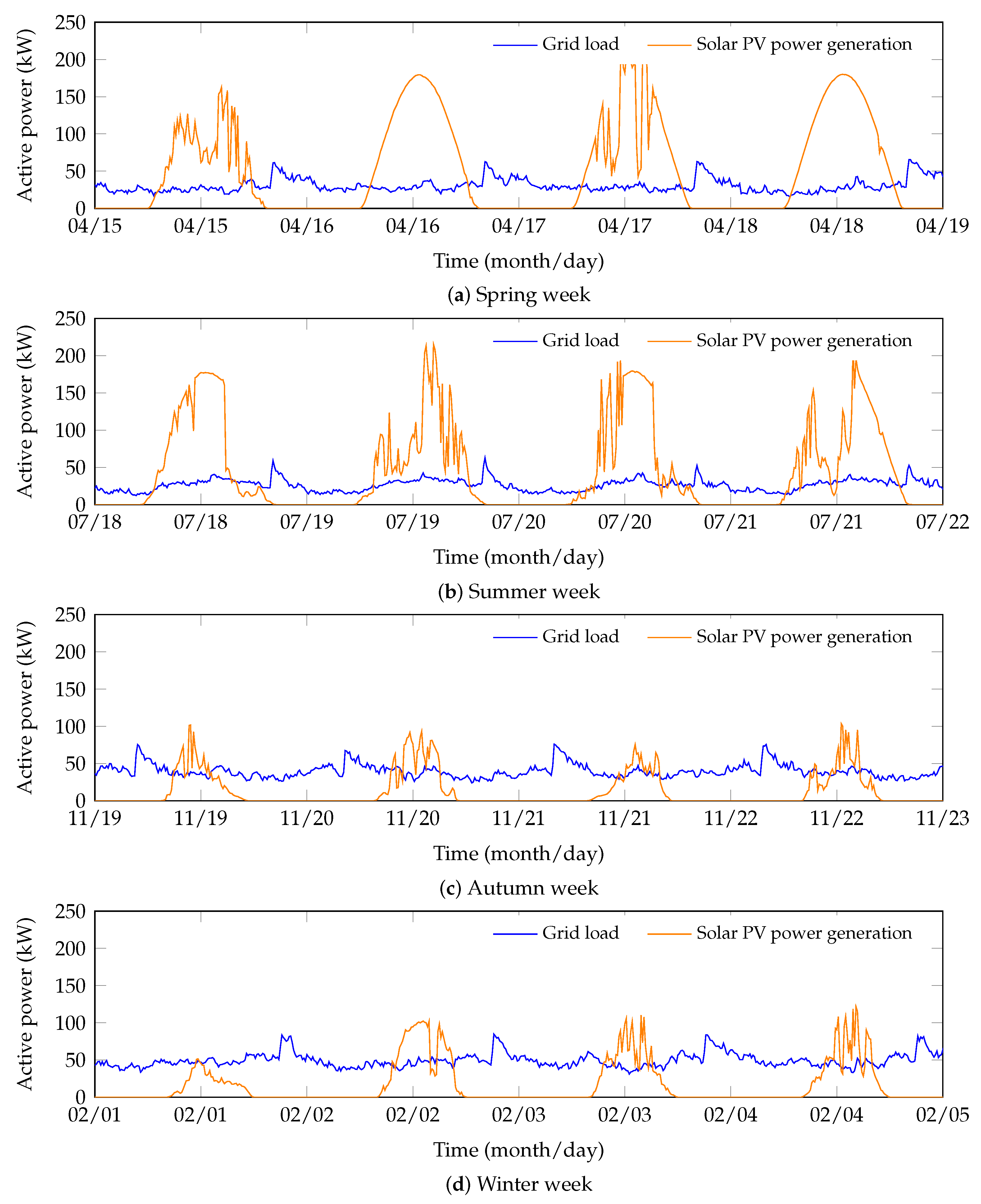
In this section, the case study, the principles of the proposed control strategy, and the models of the low-voltage power distribution grid and flexible assets used in this case study are presented.

2.1. Case Study

The simulated case study presented herein is carried out on a low-voltage power distribution grid composed of a suburban residential neighbourhood of approximately 120 households located in the Occitania region (south of France), 50 household PV installations of 4 k W each (approximately 20 m ), amounting to a total power capacity of 200 k W , a biogas plant (power capacity is 100 k W ), and a water tower (power capacity is 100 k W ). The considered solar PV power generation capacity is in reality a fourfold increase from the current installed capacity in the considered power distribution grid. The current capacity not being high enough to disrupt the smooth functioning of the power distribution grid, this increase in capacity was decided on to demonstrate the predictive control strategy’s ability to close a significant gap between power supply and demand, while maintaining the voltage levels within prescribed margins (in France, 10% for power distribution grids).
Grid load is measured at the medium-voltage/low-voltage (MV/LV) transformer level of the residential neighbourhood. Data are provided by CAHORS group, which is involved in the Smart Occitania project, and ENEDIS. Because grid load data show that the portion of reactive power remains under 5% of the apparent power, both the inductive and capacitive aspects of the power grid components are neglected. Solar PV power generation is inferred from global horizontal irradiance (GHI) measurements taken by a pyranometer installed at PROMES-CNRS, located just a few kilometres from the residential neighbourhood. Grid load and solar PV power generation data used in the case study are presented in Figure 1. Both the biogas plant and the water tower used herein match the characteristics of two real installations located in the Occitania region.

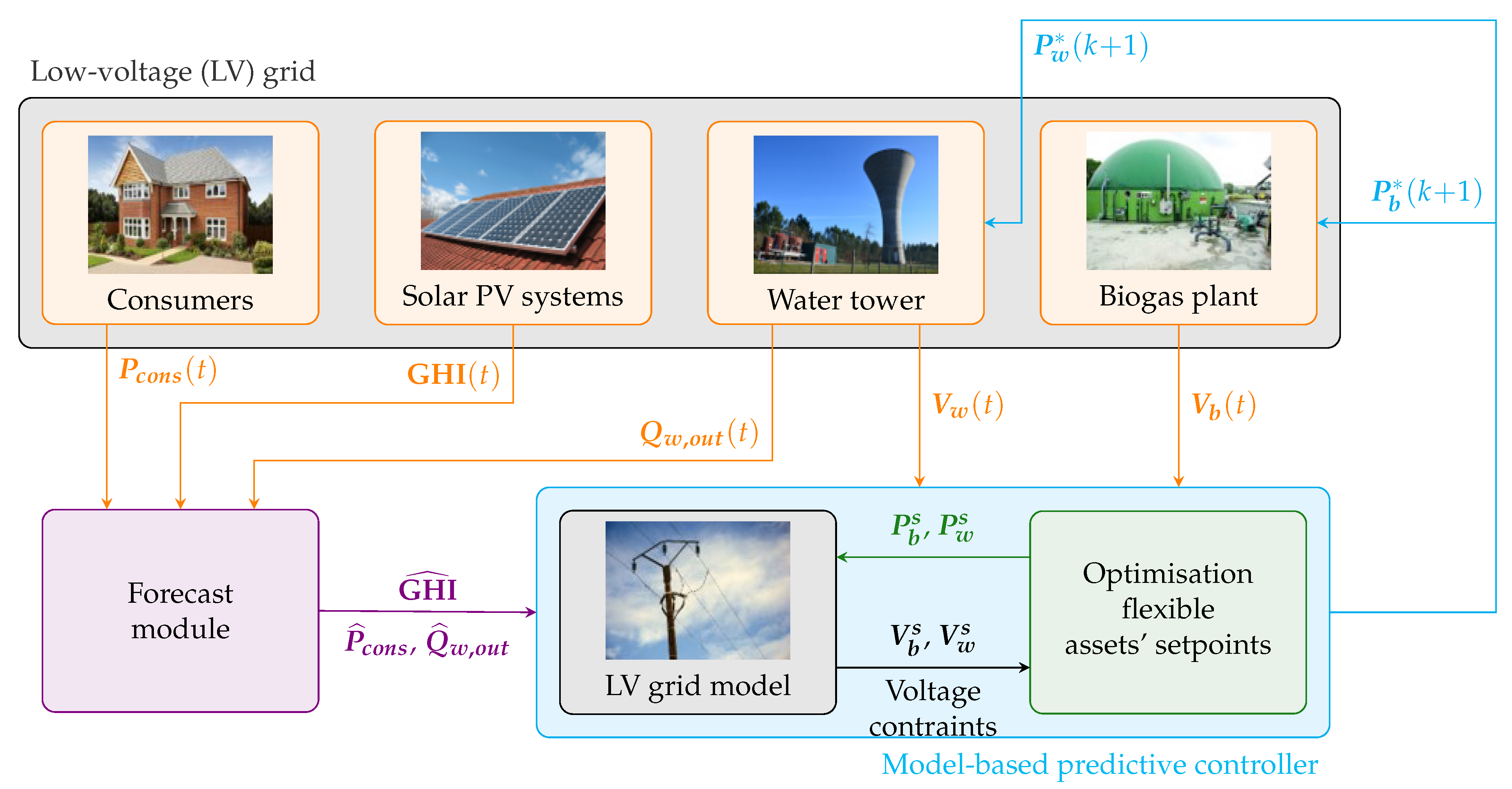
2.2. Overview of the Proposed Control Strategy

In this section, the MPC-based strategy, dubbed switch control strategy, proposed for the smart management of low-voltage power distribution grids is introduced. The principle upon which MPC is based is quite simple: a dynamic model of the system’s inner-workings, coupled with forecasts of stochastic quantities, is used to solve a constrained optimisation problem, herein the one described in Section 3.2, over a sliding window. During each timeslot, only the setpoints corresponding to the next time step are implemented. This process is reiterated at each time step. The strength of model-based predictive control is in its ability to incorporate in real time forecasts of disturbances impacting grid’s stability, namely solar PV power generation and grid load, for anticipating emerging constraints as best as possible.
In contrast to a classic operation planning where a single optimisation problem is solved and its solution implemented over a fixed horizon (e.g., a week), the rolling horizon of a MPC controller, which allows a perpetual adaptation to the enhancement of forecasts, is suitable for real-time control as the optimisation problem to be solved over a pre-defined sliding window is much less expensive. In addition, power distribution grids contain several stochastic quantities whose forecasts degrade quickly as the forecast horizon expands.
Figure 2 summarises the proposed MPC-based strategy. At each time step, the low-voltage power distribution grid model assimilates data coming from both the forecast module and the metering infrastructure concerning the biogas production at the biogas plant, water consumption affecting the stored water level in the water tower, solar PV power generation and the grid load. Then, the model evaluates the voltage constraints created in the grid and sends this information to the optimisation algorithm which attempts to find a solution for the flexible assets’ setpoints. Once the optimisation problem is solved, the first setpoint (for the following time step) is implemented. The entire process reiterates at every time step.
The proposed MPC-based control strategy, dubbed switch control strategy, is detailed in Section 3. The MINLP problem is presented and the novel formulation that solves this problem as a smooth continuous one without having recourse to relaxation is introduced.

2.3. Models

In accordance with the model-based predictive control scheme proposed in this paper for the smart management of a low-voltage power distribution grid, the models of the flexible assets (a biogas plant and a water tower) are formulated over a prediction horizon H. In the following, and for all time-dependant quantities, t { 1 , , H p } , where H p is the integer number of time slots within the prediction horizon.

2.4. Biogas Plant

Biogas plants, which are connected to low-voltage power distribution grids, are composed of bioreactors (where methane-rich biogas is produced in order to be used as fuel), storage units, and power generators.
The biogas volume in the storage unit (in m 3 ) is described as:
V b ( t + 1 ) = V b ( t ) + T 60 Q b , in ( t ) Q b , out ( t )
where T is the time step ( T = 10   min ) and Q b , in (in m 3 / h 1 ) and Q b , out (in m 3 / h 1 ) are the flow rates of biogas production entering the storage unit and biogas consumption by the power generator, respectively.
Q b , out is formulated as follows:
Q b , out ( t ) = P b ( t ) η LHV
where P b (in W ) is the plant’s active power output, η is the generator’s efficiency, and LHV (in kWh / m 3 ) is the lower heating value of the stored biogas.
P b is subject to the following constraint:
P b , m i n P b ( t ) P b , m a x
where P b , m i n and P b , m a x are the minimal and maximal power generation of the biogas plant, respectively.
Regarding the biogas volume in the storage unit ( V b ), it is subject to the following constraint:
V b , m i n V b ( t ) V b , m a x
where V b , m i n and V b , m a x are the minimal and maximal biogas storage capacities of the biogas plant, respectively.

2.5. Water Tower

Water towers, which are connected to low-voltage power distribution grids, provide pressurised potable water supply and emergency water storage for fire protection. The volume in the storage tank (in m 3 ) is described as follows:
V w ( t + 1 ) = V w ( t ) + T 60 Q w , in ( t ) Q w , out ( t )
where T = 10   min is the time step and Q w , in (in m 3 / h 1 ) and Q w , out (in m 3 / h 1 ) are the flow rates of water entering the storage tank and water consumption, respectively.
Q w , in is formulated as follows:
Q w , in ( t ) = P w ( t ) 3600 η w ρ g h
where P w (in W ) is the water pump’s active power consumption, η w is the water pump’s efficiency, ρ (in k g / m 3 ) is the water density, g (in m / s 2 ) is the gravitational acceleration, and h (in m ) is the water level in the storage tank.
Let P w , m i n and P w , m a x be the minimum and maximum power consumption values of the water tower, respectively. P w can only be set following ON/OFF commands, i.e., it is subject to the following constraint:
P w ( t ) { P w , m i n ; P w , m a x }
The water volume in the storage tank ( V w ) is subject to the following constraint:
V w , m i n V w ( t ) V w , m a x
where V w , m i n and V w , m a x are the minimal and maximal storage capacities of the water tank, respectively.

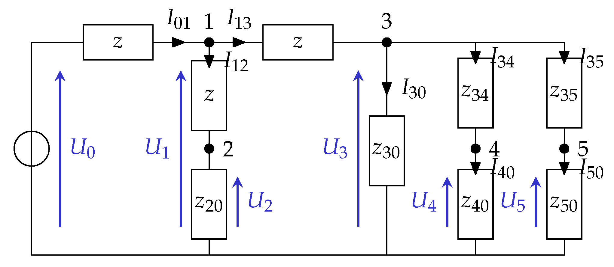
2.6. Low-Voltage Power Distribution Grid Model

The proposed control scheme operates at the MV/LV transformer level of a small-scale power distribution grid, whose equivalent electrical circuit is shown in Figure 3, in order to minimise the gap between power supply and demand. Therefore, performance of the control scheme is independent of the dispatching of distributed generation throughout the power grid.
For a given branch [ q j ] , the voltage drop between nodes q and j is given by Kirchhoff’s law:
U q ( t ) U j ( t ) z q j ( t ) I q j ( t ) = 0
where U q R H p , q { 1 , , N } , and U j R H p , j { 1 , , N } , are the voltages at nodes q and j, respectively; z q j R H p , q , j { 1 , , N } , is the line impedance between nodes q and j; and I q j R H p , q , j { 1 , , N } , is the current flowing between nodes q and j. N is the number of nodes in the considered power distribution grid.
Under the assumption that reactive power is negligible, U q is proportional to the active power consumed/produced at that node:
P q ( t ) = U q ( t ) I q ( t )
where P q R H p , q { 1 , , N } , is the active power consumed/produced at node q and I q R H p , q { 1 , , N } , is the current injected into/absorbed by node q.
In France, in low-voltage power distribution grids, the nominal voltage values for single-phase and three-phase connections are 230 V and 400 V , respectively [2]. In addition, measurements—made at the transformer level of the power distribution grid—used throughout this study correspond to means over each time step (herein T = 10 min ). Because voltage means must at all times remain within prescribed margins, q { 1 , , N } :
| U q ( t ) U n | δ U
where U n is the nominal single-phase voltage value for all grid nodes and δ U is the prescribed margin of voltage variations with respect to the nominal value (in France, 10% for power distribution grids). Here, U n = 230 V and δ U is set to be 10% of U n , that is δ U = 23 V .
Hereinafter, let us define the following bounds:
U m i n = U n δ U
and
U m a x = U n + δ U
For the equivalent electrical circuit of the low-voltage power distribution grid of the case study (Figure 3), Equations (9) and (10) lead to the following equation set:
U 3 ( t ) U 4 ( t ) + z ( t ) P b ( t ) U 4 ( t ) = 0
U 1 ( t ) U 2 ( t ) z ( t ) P w ( t ) U 2 ( t ) = 0
U 3 ( t ) U 5 ( t ) + z ( t ) P PV ( t ) U 5 ( t ) = 0
U 1 ( t ) + U 4 ( t ) + U 5 ( t ) 3 U 3 ( t ) z ( t ) P cons ( t ) U 3 ( t ) = 0
U 3 ( t ) 3 U 1 ( t ) + U 2 ( t ) + U n = 0
where P PV and P cons are the solar PV power generation and the grid load, respectively.

3. Control Strategy

In this section, the switch control strategy and the reference strategies—these strategies are based on a relaxation of the MINLP problem—are presented. Because solar PV power generation and grid load forecasting errors are assumed null, the difference in performance between these strategies can only be traced back to differences in problem formulations, since data are identical. The switch control strategy is taken because the focus of this paper is to demonstrate the efficiency of the new problem formulation and to evaluate its performance.
This section starts with formulating the problem as a standard MINLP one. Then, the new problem formulation allowing to treat the optimisation problem as a smooth continuous one without having recourse to relaxation is introduced. The section ends with a presentation of the two reference strategies with which the proposed scheme’s performance is evaluated.

3.1. MINLP Formulation

In the scope of this work, the flexible assets are operated by third parties. The water tower is operated using an ON/OFF controller, a hard constraint by which the power distribution grid control scheme must abide. The integer values of the water tower control setpoint makes the problem a MINLP one [43]. In this section, the aforementioned MINLP problem formulation is presented. In the following, and for all time-dependant quantities, t { 1 , , H p } . Let H be the prediction horizon such that H = H p · T , where H p is the integer number of time slots within the prediction horizon, P cons R H p is the grid load (in W ), and P PV R H p is the solar PV power generation (in W ). The decision variables are P b R H p and P w R H p , which represent the active power setpoints for the biogas plant generation and the water tower consumption. The standard way of integrating acceptable voltage fluctuation margins into the problem would be to write the Kirchhoff laws dictating them as nonlinear constraints. However, in this paper, things are done differently. Voltage variables are introduced so the optimisation model solves the solution for power setpoints and the voltage values across the low-voltage power distribution grid at the same time.
Moreover, voltages are incorporated as optimisation variables and nonlinear constraints described by Kirchhoff laws are turned into linear ones. This version of the problem alleviates its complexity by reducing the number of nonlinear constraints it contains. The voltage variation between nodes q and j of a power distribution grid at time step t is described as follows, q , j { 1 , , N } :
B q j ( t ) = U q ( t ) U j ( t ) z q j ( t ) · P j ( t ) U j ( t )
Kirchhoff laws ensure that, at every time step, the following condition is verified, q , j { 1 , , N } :
B q j ( t ) = 0
Current variables are eliminated using Kirchhoff’s laws. As a result, K t is defined to represent voltage variations across the power distribution grid at a given time step t as a function of the powers injected/absorbed at each node in the following manner:
K t : ( R , R , R N ) R M
( P b ( t ) , P w ( t ) , υ ( t ) ) B ( t )
such that
υ ( t ) = U 1 ( t ) U 2 ( t ) U N ( t ) T
where M is the number of vertices in the connected loopless graph equivalent to the electrical circuit in question and B is made up of M non-redundant elements B q j .
Now, let X be the following matrix:
X = P b P w υ
where X R H p × ( N + 2 ) .
The problem aims to close the gap between power supply and demand in a power distribution grid. To do so, third-party-owned biogas plant and water tower must be managed in such a way that their power generation/consumption balances out the discrepancies in the grid’s supply/demand equilibrium.
As a result, the objective function is formulated as follows:
f o b j ( X ) = t = 1 H p | P PV ( t ) + P b ( t ) P cons ( t ) P w ( t ) | 2
The optimisation problem that takes into account the ON/OFF controller specificity of the water tower is:
X * = arg min X f o b j ( X )
with biogas plant setpoint boundaries
P b , m i n P b ( t ) P b , m a x
and voltage boundaries, q { 1 , , N }
| U q ( t ) U n | δ U
subject to the following constraints:
  • Water tower setpoint constraint
    P w ( t ) { P w , m i n , P w , n o m }
  • Linear inequality constraints, q { 1 , , N }
    V b , m i n V b ( t ) V b , m a x
    V w , m i n V w ( t ) V w , m a x
    | U q ( t ) U n | δ U
  • Nonlinear equality constraints
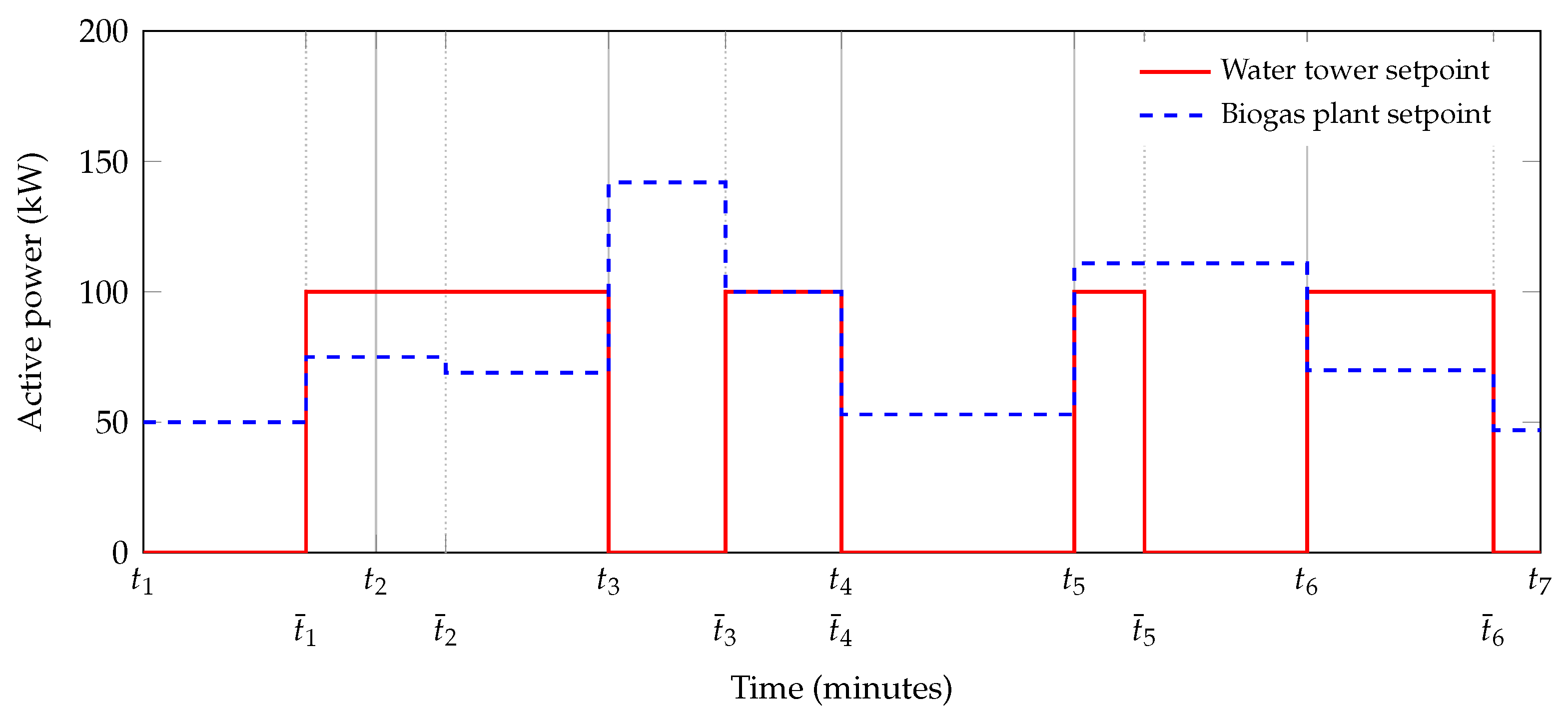
    K t ( P b ( t ) , P w ( t ) , υ ( t ) ) = 0

3.2. Switch Control

In this section, the new problem formulation proposed by PROMES-CNRS, allowing the ON/OFF control of the water tower without using MINLP, is introduced. A post-treatment is then presented (the post-treatment algorithms are detailed in Appendix A) to make the solution more suitable for real implementation. Lastly, an explanation is provided of the addition of constraints into the problem in favour of the reduction of the number of variables. The problem as formulated in Section 3.1 presents a major challenge in the form of the MINLP setting due to the water tower ON/OFF controller. This setting is complex and computationally expensive, an especially troublesome trait for real-time applications such as the one addressed in this paper. The usual route taken in the literature to bypass the difficulties of MINLP are relaxation techniques [38,47,48]. Instead, the approach presented in this paper does not relax the problem but proposes a different formulation that allows the mixed-integer problem to be solved as a smooth nonlinear optimisation by optimising the timing of the integer variable’s transition from one integer value to another. To the authors’ knowledge, even though this technique comes from parameterised optimal control theory, it has not yet been implemented for this type of application. However, a similar approach was implemented by Salas et al. [49] to determine optimal planning strategies for concentrated solar power plants via pre-scenarios. The reader can note that the constraints given by Equation (33) are non-convex. Therefore, only local optimality can be expected, even if the integer constraints (29) are relaxed. As a result, optimality bounds and analysis of the results must be considered under this setting as heuristic results.
The MINLP setting due to the water tower ON/OFF controller greatly increases the computational complexity of the optimisation problem. To circumvent this issue, this work proposes a new formulation of the optimisation problem in order to solve it as a continuous one. This is done by exchanging the discrete optimisation variable P w with a real-valued one t ¯ R H p that designated the instant between two time steps at which the water tower’s setpoint switches between its two discrete values (i.e., P w , m i n and P w , m a x ). It follows that, at the same instant, the biogas plant’s setpoint also switches between two values within the interval [ P b , m i n , P b , m a x ] .
Let us denote X = P b , ON P b , OFF t ¯ U ON , q U OFF , q T , where P b , ON R H p and P b , OFF R H p form the biogas plant setpoint as follows:
P b ( τ ) = P b , ON ( τ ) , τ [ t i , t i + t ¯ i ] P b , OFF ( τ ) , τ [ t i + t ¯ i , t i + 1 ]
U ON , q R ( H p · N ) and U OFF , q R ( H p · N ) , q { 1 , , N } , form the voltages in the grid:
U q ( τ ) = U ON , q ( τ ) , τ [ t i , t i + t ¯ i ] U OFF , q ( τ ) , τ [ t i + t ¯ i , t i + 1 ]
At each time step, the problem can be solved assuming that the first state of the water tower is always ON. In some extreme cases, this assumption may induce some issues of implementability with volume constraints, which are tackled in a post-treatment phase (see Appendix A). However, this simplification reduces the complexity of the model without sacrificing much performance.
Figure 4 gives an example of what the water tower and biogas plant setpoints would look like with the switch control formulation. Note that the transition between states does not only occur at the beginning of each time step.
The objective function is formulated as follows:
f o b j ( X ) = i = 0 H p 1 t i t i + t ¯ i S ON ( τ ) d t + t i + t ¯ i t i + 1 S OFF ( τ ) d t
with
S ON ( τ ) = | P PV ( τ ) + P b ( τ ) P cons ( τ ) P w , m a x | 2
and
S OFF ( τ ) = | P PV ( τ ) + P b ( τ ) P cons ( τ ) P w , m i n | 2
The problem is then formulated as follows:
X * = arg min X f o b j ( X )
subject to, i { 1 , , H p } and q { 1 , , N } :
  • Biogas plant power bounds
    P b , m i n P b , ON ( τ ) P b , m a x
    and
    P b , m i n P b , OFF ( τ ) P b , m a x
  • Switch time bounds
    0 t ¯ i T
  • Biogas volume constraints
    V b , m i n V b ( t ) V b , m a x
  • Water volume constraints
    V w , m i n V w ( t ) V w , m a x
  • Voltage constraints
    t ¯ i · K t ( P b , ON ( τ ) , P w , m a x , U ON , q ( τ ) ) = 0
    ( T t ¯ i ) · K t ( P b , OFF ( τ ) , P w , m i n , U OFF , q ( τ ) ) = 0
    | U ON , q ( τ ) U n | δ U
    | U OFF , q ( τ ) U n | δ U
K t , which is formulated as a function of the power injected or absorbed by the power grid nodes, as defined in Equation (22), deals with voltage variations across the low-voltage power distribution grid. Two sets of constraints guarantee that Kirchhoff’s laws are upheld in both sub-intervals of each time step (Equations (45) and (46)). The equation set depicting voltage variations across the power distribution grid is multiplied by t ¯ i (Equation (45)) and by T t ¯ i (Equation (46)) using for each interval appropriate values of biogas plant and water tower setpoints, with the aim of ensuring that only one constraint is activated in case of extreme values of t ¯ i . If t ¯ i = 0 , Equation (45) is removed. This reflects the fact that the water tower is turned off at the beginning of time step i. If t ¯ i = T , Equation (46) is removed since the water tower remains on for the whole duration of time step i.
Two other sets of constraints account for voltage variations in both states of the power distribution grid within each time step (Equations (47) and (48)). While depicting the same physical constraints, this optimisation problem formulation has a bigger feasible set than the mixed-integer nonlinear programming one (see Section 3.1). As a consequence, the global optimum of this formulation is guaranteed to be equal or better than the one of the MINLP formulation.

3.2.1. Post-Treatment

The problem treated in this section splinters the regularly-split time horizon into uneven intermediate intervals. As a result, the power setpoints provided by the optimisation algorithm may present very small pulses which perfect the objective function minimisation aspect but compromise the implementability of the solution. Moreover, small pulses may also appear when trying to set the switch time to an extreme value. For all intents and purposes, a water tower setpoint which stipulates that the pump be turned on for 30 s , for instance, makes little to no practical sense. This issue calls for a post-treatment to eliminate small pulses, while still upholding all constraints.
At each iteration i of the optimisation process, the determined switching time t ¯ i is examined: if the pulse during which the pump is turned on is too short with respect to a pre-defined threshold, then the pulse is eliminated, provided that the volume constraints would still hold. Analogously, if said pulse surpasses the post-treatment threshold, the algorithm attempts to extend it to the full 10-min interval, if volume constraints permit it. Moreover, a second post-treatment is applied to join two adjacent pulses when possible. This enhances the implementability of the solution as the algorithm tries to minimise the number of transitions of the water tower setpoint from one state to another, when the volume constraints allow it. The post-treatment algorithms are detailed in Appendix A.

3.2.2. Additional Constraints

In the remainder of this section, all quantities written in a bold font are time-dependent. However, for clarity’s sake, notations do away with time indices and time dependency is implicit. To alleviate the computational burden of the problem, it is advantageous to reduce the number of optimisation variables. In this case study, this is rendered possible by the reformulation of Equations (14)–(18), which can then be written as follows:
U n U 1 = z P w U 2 + P cons U 3 + P b U 4 + P PV U 5
and
U 1 U 3 = z P cons U 3 + P b U 4 + P PV U 5
such that
U 2 = U 1 + U 1 2 4 z P w 2
U 4 = U 3 + U 3 2 + 4 z P b 2
U 5 = U 3 + U 3 2 + 4 z P PV 2
where Equations (51)–(53) are solutions to Equations (14)–(16), respectively.
The discarded solutions to the quadratic equations are the ones that would provide voltage values that make no physical sense. At this stage, it becomes clear that there are merely two voltage variables ( U 1 and U 3 ) in the optimisation problem. However, in reality, voltages U 2 , U 4 , and U 5 are still expected to be within the bounds described in Equation (11). As a result, these bounds infer additional constraints on variables U 1 and U 3 . In the following, these constraints are determined.
  • Constraints inferred by bounds of U 2 : from Equation (51), it is trivial that U 2 U 1 . As a result, U 2 U m a x is redundant. As for the lower bounds, using Equation (51):
    U m i n U 2
    U m i n U 1 + U 1 2 4 z P w 2
    2 U m i n U 1 U 1 2 4 z P w
    Since 2 U m i n U m a x , 2 U m i n U 1 0 . Then:
    ( 2 U m i n U 1 ) 2 U 1 2 4 z P w 2
    U m i n 2 + z P w U m i n U 1 [ Additional constraint 1 ]
  • Constraints inferred by bounds of U 4 : from Equation (52), it is trivial that U 4 U 3 . As a result, U 4 U m i n is redundant. As for the upper bound, using Equation (52):
    U m a x U 4
    U m a x U 3 + U 3 2 + 4 z P b 2
    2 U m a x U 3 U 3 2 + 4 z P b
    ( 2 U m a x U 3 ) 2 U 3 2 + 4 z P b 2
    U m a x 2 z P b U m a x U 3 Additional constraint 2 ]
  • Constraints inferred by bounds of U 5 : analogously to the constraints inferred by U 4 , and by using Equation (53), it can be easily demonstrated that U 5 U m i n is redundant. As a result:
    U m a x 2 z P PV U m a x U 5 [ Additional constraint 3 ]

3.3. Reference Strategies

In this section, the two reference strategies (i.e., an operation planning of the flexible assets over the considered one-week periods, see Section 3.3.1, and a relaxed MPC scheme, see Section 3.3.2) are briefly presented. Both strategies are based on a relaxation of the MINLP problem described in Section 3.1.
By relaxing the problem formulation, the ON/OFF constraint of the water tower controller is lifted, and it is assumed that water consumption may have any value within a feasible interval. Therefore, the relaxed problem is formulated in the same way as the MINLP one except for Equation (29), representing the ON/OFF characteristic of the water tower setpoint. Equation (29) is replaced by:
P w , m i n P w ( t ) P w , m a x

3.3.1. Weekly Planning

The first reference strategy is an operation planning of the flexible assets over the one-week periods considered in this paper. Over an entire week, the relaxed optimisation problem is solved once and then the solution is implemented. Although this type of planning strategies is not frequently used, it is not uncommon for installations such as biogas plants. In this paper, solar PV power generation and grid load forecasting errors are assumed null (the difference in performance between the considered strategies can therefore only be traced back to differences in problem formulations). The purpose of using this weekly planning strategy, assuming forecasting errors to be null, is to serve as an upper bound for the efficiency of the control strategy in closing the power supply/demand gap.

3.3.2. Relaxed MPC Scheme

The second reference strategy is a MPC scheme based on the relaxed problem formulation. In this case, the proposed MPC scheme, based on a new formulation of the problem described herein, is compared to a relaxed MPC scheme that is given ample freedom to change the water tower setpoint between its two extreme values (i.e., P w , m i n and P w , m a x ).

4. Results and Analysis

In this section, a performance analysis of the switch control strategy (see Section 3.2) is carried out. These performances are compared to those of the weekly planning strategy and the MPC scheme based on the relaxed optimisation problem, both explained in Section 3.3. First, the results yielded by the weekly planning using all four datasets are presented. Then, a sensitivity analysis is conducted in order to assess the impact of the MPC’s sliding window length on its performance. Lastly, a sliding window is chosen based on the aforementioned sensitivity analysis and a detailed examination of its results is done. All results presented in this paper were obtained using MATLAB 2018a (MathWorks, Natick, MA, USA).

4.1. Weekly Planning Performance

The weekly planning of the flexible assets’ operation is conducted in four different scenarios: each corresponding to a “season-typical” week (see Figure 1). Results displayed hereinafter showcase the reduced gap between supply and demand obtained through this planning, as well as flexible asset setpoints and corresponding storage volumes, compared to the initial case.
It is interesting to note that the dimensioning of flexible asset storage units is an influential factor in itself. As it stands, the hard volume constraints of storage units are prioritised by the algorithm over the minimisation of the supply/demand gap. As a result, when the upper bound of stored biogas volume is reached, the generator kicks in to burn the extra biogas to avoid discarding it into the atmosphere or increasing the storage unit pressure. When the lower bound is reached, the setpoint of power generation is reduced in order to maintain the minimum required volume in storage. Similarly, the water tower’s pump is automatically triggered when the lower volume bound is reached in order to maintain the minimum required volume in storage and is automatically shut down when the maximum water volume is reached. This can sometimes be in conflict with the grid stability’s best interest, as it may be necessary to turn on the distributed generator when the grid is already experiencing overvoltage due to excess energy flowing through its lines. It may also be necessary for the storage system to consume electricity at times when the grid is at risk of experiencing undervoltage phenomena. Asset dimensioning is not addressed in this paper, but several works exist in the literature to tackle the question of optimal dimensioning and allocation of distributed generators in power distribution grids [28,50,51].
Table 1 recapitulates the values of the power supply/demand gap procured by the weekly planning with all four sets of data, where f o b j , i n i t i a l and f o b j , f i n a l are the initial and final objective function values, respectively. When formulating the optimisation problem, the square of the objective function is used to ensure that the algorithm suppresses sharp fluctuations of its values and gives as smooth a variation as possible. The results show that, in all four cases, there is a significant reduction in the supply/demand gap with respect to the initial case, the biggest of which occurs during winter.
Depending on the season, the initial gap between supply and demand within the considered low-voltage power distribution grid (modelled by the objective function value) differs: the gap is higher in warmer seasons (spring and summer) as the solar resource, and therefore solar PV power generation, is substantial. This is typical for the Mediterranean climate. Indeed, the results show that the power distribution grid is unable to absorb the excess of power generation during spring and summer, as the final objective function is reduced by 26.5% and 26.1%, respectively, whereas it is reduced by 46.9% for winter and 41.5% for autumn. The weekly planning scheme presented in this section, using the relaxed problem formulation and assuming perfect forecasts, is considered as the “ideal case” throughout the rest of the paper.

4.2. Sensitivity Analysis

To assess the impact of the sliding window size on the MPC-based strategy’s performance, both the relaxed problem and the switch control are implemented with sliding window size ranging from 1 to 24 h over four season-representative weeks. The results of these simulations are discussed herein. The interesting question being investigated is: What is the most appropriate length of this sliding window that would allow efficient control of the power distribution grid without taking on unnecessary computational burdens? To determine an answer, a sensitivity analysis of the impact of the sliding window size on the performance of the MPC algorithm is carried out. The considered metrics are the objective function’s final value and the computational complexity, measured in the total number of objective function evaluations needed for the algorithm to reach a solution.
Figure 5 displays the evolution of the power supply/demand gap with respect to lengths of the sliding window ranging from one to 24 h, for both the relaxed problem and the switch control. The weekly planning obtained through the relaxed problem assuming perfect forecasts serves as a reference point to evaluate the MPC scheme’s accuracy. For all four seasons, it can be seen that the same behaviour is reproduced. As the sliding window length increases, the final objective function value decreases and moves towards the ideal value without reaching it. For small window lengths, the switch control provides identical values to those of the relaxed problem. For larger windows, however, the switch control’s values still follow the relaxed problem’s quite well but a small gap starts to appear between the two.
Considerable reductions in the power supply/demand gap are already obtained with a 1-h sliding window size for the MPC scheme, followed by gradual improvements as the window size increases. These improvements seem, at first glance, to stabilise relatively quickly. A closer look is provided by Figure 6, revealing a more pronounced difference between results of MPC schemes with various sliding window sizes, though the incremental change remains small when compared to reductions made to the power supply/demand gap using the 1-h window with respect to the initial values.
The scheme’s goal is real-time monitoring and control of low-voltage power distribution grids. Thus, it stands to reason that computational cost would be a cardinal criterion. Therefore, a compromise must be made between the algorithm’s qualitative results and its computational cost. To do so, an examination of the evolution of the computational cost required by the optimisation algorithm is carried out with respect to the length of the sliding window of the MPC-based strategy. Figure 7 shows the computational cost of the implementation of an iteration of the MPC scheme with varying lengths of the sliding window in order to assess the computational burden for the relaxed problem and the switch control. Herein, as opposed to simply registering the time consumed by the MPC scheme’s implementation, the computational complexity is quantified by the overall number of objective function evaluations per window. This metric is provided as an output argument of the optimisation function fmincon of MATLAB, which has been selected because it provided the best compromise between quality of results, computational cost, and simplicity of implementation. fmincon is based on interior point algorithm. The application aims at real-time control of power distribution grid, with a time step of 10 min. As a result, strict limitations are imposed on the sophistication of the numerical solver. Of course, fmincon does not guarantee convergence to a global minimum. However, for this type of applications, a local minimum that allows satisfactory enhancement of the objective function’s final value is acceptable (herein, this translates into reduction of the unbalance between power supply and demand within the considered low-voltage power distribution grid).
For a given computer and given operating conditions, the algorithm’s speed mirrors a combination of two criteria: the number of function evaluations it performs and the number of optimisation variables, which is proportional to the length of the sliding window. This allows for a more objective rendering of the algorithm’s computational complexity that is not clouded by the characteristics of a specific computer. Figure 7 shows that the switch control’s computational complexity remains underneath that of the relaxed problem up to a certain window length, then it surpasses it. Which means that, up to a certain, relatively large, window length, the switch control is not only more realistic but is also less computationally expensive than the relaxed problem.
Despite the presence of some outliers, the growing tendency of computational complexity is clear and expected. Its main cause is the number of optimisation variables, which is proportional to the length of the sliding window. The main observation is that, for longer windows, a high percentage of the function evaluations serves to improve upon values given by the previous windows by only a small fraction of the objective function’s initial value. In gradient-based descendant methods, particularly interior-point methods, this is very common due to the trade-off between convergence criteria and accuracy. For further details about convergence rates and computational complexity of interior-point methods, the reader is referred to [52] (and the references therein).
As of the 14-h sliding window, the improvement of the final objective function value with respect to the initial value is practically constant. To avoid undue computational burden caused by enlarging the sliding window size with little performance gain, the 14-h sliding window is chosen going forward as the best compromise between the aforementioned performance criteria.

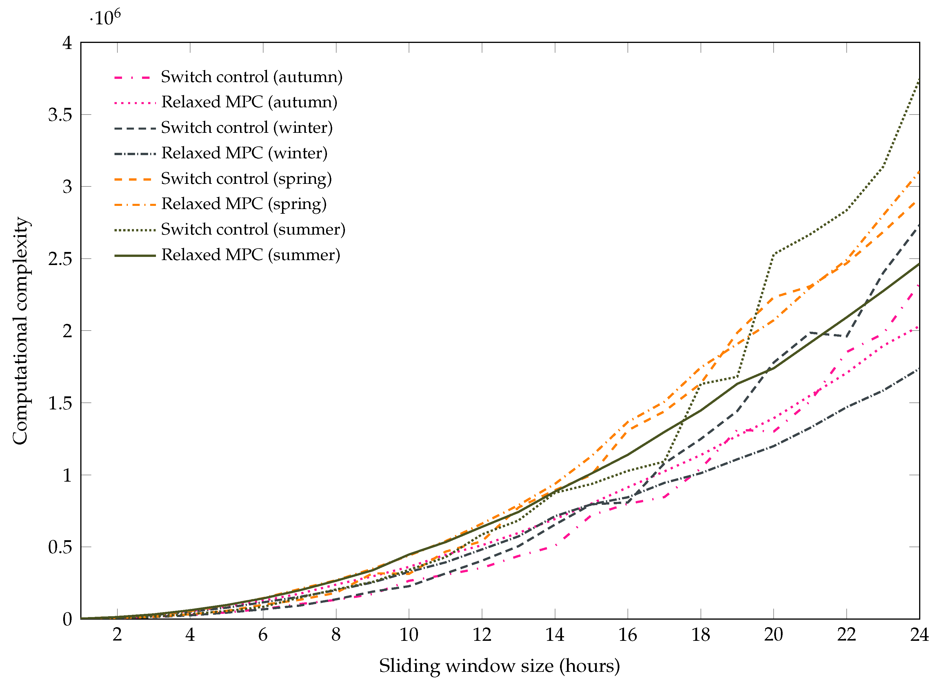
4.3. Switch Control Performance

In this section, the results provided by the switch control scheme are examined. A 14-h sliding window is considered. The initial case represents the classical operation modes of both flexible assets: through the water tower ON/OFF controller that allows the pump the system is equipped with to fill the tank whenever it is at a lower threshold and stops when reaching the upper threshold, and constant power generation for the biogas plant, in line with the facility’s steady flow of biogas production. Table 2 details the objective function’s final values given by the proposed switch control scheme with a 14-h sliding window, with respect to the objective function’s initial values.
Figure 8 shows the gap between power demand and supply in the considered low-voltage power distribution grid before and after implementing the switch control scheme with a 14-h sliding window with respect to the initial case and the planning strategy. The results are observed for four “season-typical” weeks, with varying behaviours of grid load and solar PV power generation, as illustrated in Figure 1. For all four considered weeks, significant smoothing of the supply/demand gap is observed with respect to the initial case. This is especially visible for the warm seasons (April and July) where the large midday peaks due to high levels of solar PV power generation are remarkably reduced, although some previously inexistent dips are created.
It should be noted that the influence of the post-treatment algorithm on performance is evaluated. In fact, the post-treatment algorithm is called, on average, 96% of the time during a one-week simulation to eliminate or extend a pulse in the water tower’s setpoint at the following time step. Although this procedure results in smoother setpoints for the flexible assets, thus boosting the solution’s implementability, it has little impact on the power supply/demand gap, which is degraded by about 4%.
The fact that the scheme that uses a post-treatment algorithm provides smoother setpoints than the one that does not while the supply/demand curve for both schemes remain virtually identical suggests that the main contribution of this post-treatment is in fact in flipping the order of the states within a time-step to have a more implementable overall setpoint. More details about the inner-workings on the post-treatment algorithm are provided in Appendix A. Another noteworthy observation is that the computational burden is increased by 12%, on average, by the post treatment.
The deployment of distributed generation and its penetration in low-voltage power distribution grids is creating new challenges in terms of monitoring and control. That being said, this type of power generation opens the door to new ways of guaranteeing the grid stability and quality of service. To this end, advanced metering infrastructures and forecasting algorithms are particularly valuable tools.

5. Conclusions and Outlook

In this paper, a control strategy, dubbed switch control, is proposed for smart management of suburban low-voltage power distribution grids with significant penetration of solar photovoltaic power generation. A simulated case study is carried out on a residential neighbourhood located in the Occitania region (southern France). Two flexible assets—a biogas plant and a water tower—are operated. This strategy consists in a model-based predictive control (MPC) scheme aiming to close the gap between power supply and demand, in accordance with voltage constraints and the flexible assets’ operational constraints.
The mixed-integer nonlinear programming (MINLP) setting due to the water tower ON/OFF controller greatly increases the computational complexity of the optimisation problem. Thus, one of the contributions of this paper is the new formulation allowing the MINLP problem to be solved as a smooth continuous one without having recourse to relaxation. In addition, the analysis of the results proves the control strategy’s potential for closing the power supply/demand gap. In fact, this gap is significantly lower than the one observed using the flexible assets’ default operating strategies (without any optimisation). In this sense, the strategy proposed herein is a step towards low-voltage power distribution grids capable of integrating renewable-energy-based power generation, whose aim is meeting power demand while maintaining stability and quality of service. In addition, the results highlight that MPC has potential for upper-level power flow management and curtailment of voltage fluctuations in low-voltage power distribution grids.
Improvements upon this work include the modification of the objective function to smooth out the flexible assets’ setpoints without having recourse to a post-treatment algorithm. In addition, forecasts of disturbances, namely solar PV power generation and grid load, impacting grid’s stability will be incorporated, in real time, with the aim of better anticipating emerging constraints. Gaussian process regression models have been developed. The MPC scheme’s robustness to forecasting errors will be investigated.

Author Contributions

Methodology, N.D. and D.S.; formal analysis, N.D. and D.S.; investigation, N.D. and D.S.; writing—original draft preparation, N.D.; writing—review and editing, S.G.; supervision, J.E., S.T. and S.G.; project administration, S.G.; funding acquisition, S.G. All authors have read and agreed to the published version of the manuscript.

Funding

This research was funded by the French agency for ecological transition (ADEME).

Institutional Review Board Statement

Not applicable.

Informed Consent Statement

Not applicable.

Data Availability Statement

Not applicable.

Acknowledgments

The authors would like to thank the French agency for ecological transition for its financial support. We also thank all the academic and industrial entities involved in the Smart Occitania project for their contribution to this work and the Universidad de O’Higgins for its financial support during the stay of Nouha Dkhili in Chile. Powered@NLHPC: This research was partially supported by the supercomputing infrastructure of the NLHPC (ECM-02).

Conflicts of Interest

The authors declare no conflict of interest.

Abbreviations

The following abbreviations are used in this manuscript:
DGDistributed generation
GHIGlobal horizontal irradiance
MINLPMixed-integer nonlinear programming
MPCModel-based predictive control
LVLow voltage
MVMedium voltage
PVSolar photovoltaics

Appendix A. Post-Treatment Algorithm

To ensure the implementability of the flexible asset setpoints, particularly the water tower that switches between two extreme setpoint values, a post-treatment algorithm is carried out. Please refer to the nomenclature list for the meaning of the variables used in equations.
Throughout the Appendix, all quantities written in a bold font are time-dependent, but, for clarity’s sake, notations do away with time indices. Moreover, the procedure presented herein is implemented at each time step. Thus, time-dependent variables correspond to the current time step, except for V b and V w , which correspond to the biogas volume and the water volume at the end of the precedent time step, i.e., at time step t, V b and V w correspond to V b ( t 1 ) and V w ( t 1 ) . In other words, V b and V w are treated as the initial conditions for the current time step.
At each iteration i of the optimisation process, the determined switching time t ¯ i is examined: if the pulse during which the pump is turned on is too short with respect to a pre-defined threshold, then the pulse is eliminated, provided that the volume constraints would still hold. Analogously, if said pulse surpasses the post-treatment threshold, the algorithm attempts to extend it to the full 10-min interval, if volume constraints permit it. Different quantities are introduced for the biogas plant volume constraints. These quantities are listed hereinafter.
  • V b , down is the stored biogas volume in the biogas plant’s storage unit at the end of the current time step if the pulse is eliminated, i.e., if in case the pump is not turned on in the current time step.
    V b , down = V b + Q b , in T 60 K b P b , OFF
    with:
    K b = T 60 LHV η b
  • V b , up middle is the stored biogas volume in the biogas plant’s storage unit at switching time t ¯ i of the current time step if the duration of the pulse is extended to equal the pre-defined threshold, i.e., if t ¯ i = ϵ .
    V b , up middle = V b + ϵ Q b , in T 60 K b P b , ON
  • V b , up end is the stored biogas volume in the biogas plant’s storage unit at the end of the current time step if the duration of the pulse is extended to equal the pre-defined threshold, i.e., if t ¯ i = ϵ .
    V b , up end = V b + Q b , in T 60 ϵ K b P b , ON ( 1 ϵ ) K b P b , OFF
  • V b , up is the stored biogas volume in the biogas plant’s storage unit at the end of the current time step if the pulse is extended, i.e., if the pump is turned on during the entire time step.
    V b , up = V b + Q b , in T 60 K b P b , ON
  • V b , down middle is the stored biogas volume in the biogas plant’s storage unit at switching time t ¯ i of the current time step if the duration of the pulse could not be extended and is shortened to t ¯ i = 1 ϵ .
    V b , down middle = V b + ( 1 ϵ ) Q b , in T 60 P b , ON K b
  • V b , down end is the stored biogas volume in the biogas plant’s storage unit at the end of the current time step if the duration of the pulse could not be extended and is shortened to t ¯ i = 1 ϵ .
    V b , down end = V b + Q b , in T 60 ( 1 ϵ ) K b P b , ON ϵ K b P b , OFF
The following quantities are introduced for the water tower volume constraints:
  • V w , down is the stored water volume in the water tower’s tank at the end of the current time step if the pulse is eliminated, i.e., in the case the pump is not turned on in the current time step.
    V w , down = V w Q w , out T 60
  • V w , up middle is the stored water volume in the water tower’s tank at switching time t ¯ i of the current time step if the duration of the pulse is extended to equal the pre-defined threshold, i.e., if t ¯ i = ϵ .
    V w , up middle = V w ϵ Q w , out T 60 + 100 K w
    with:
    K w = T 60 η w
  • V w , up end is the stored water volume in the water tower’s tank at the end of the current time step if the duration of the pulse is extended to equal the pre-defined threshold, i.e., if t ¯ i = ϵ .
    V w , up end = V w Q w , out T 60 + 100 ϵ K w
  • V w , up is the stored water volume in the water tower’s tank at the end of the current time step if the pulse is extended, i.e., if the pump is turned on during the entire time step.
    V w , up = V w Q w , out T 60 + 100 K w
  • V w , down middle is the stored water volume in the water tower’s tank at switching time t ¯ i of the current time step if the duration of the pulse could not be extended and is shortened to t ¯ i = 1 ϵ .
    V w , down middle = V w ( 1 ϵ ) Q w , out T 60 + 100 K w
  • V w , down end is the stored water volume in the water tower’s tank at the end of the current time step if the duration of the pulse could not be extended and is shortened to t ¯ i = 1 ϵ .
    V w , down end = V w Q w , out T 60 + 100 ( 1 ϵ ) K w
At each time step, the first setpoint undergoes a treatment before it is implemented and later fed to the controller for future time steps. The treatment concerns the switching time t ¯ i [ 0 , 1 ] and infers modifications of the other setpoint variables: if the switching time t ¯ i is smaller than the pre-defined threshold ϵ , it may be set to three possible values, i.e., zero, ϵ , or t ¯ i , in that order of priority. The steps made in this case are given by Algorithm A1. If the switching time t ¯ i is bigger than the pre-defined threshold ϵ , it may be set to three possible values: 1, 1 ϵ , or t ¯ i , in that order of priority. The steps made in this case are given by Algorithm A2.
Algorithm A1: Post-Treatment Algorithm 1, Part 1.
Energies 14 01773 i001
Algorithm A2: Post-Treatment Algorithm 1, Part 2.
Energies 14 01773 i002
This choice depends on whether the volume constraints of both flexible assets hold. These constraints are guaranteed to hold in the last case by the preceding optimisation algorithm. Then, to further increase implementability of the solution, the possibility of re-arranging the positions of pulses within their respective time steps is studied. This stems from the fact that, within a time step, the optimisation variable is the duration of the pulse and not its position. In other words, within a time step, as long as the water tower is turned on for the same amount of time as what has been determined thus far, whether it is turned on in the beginning of the time step or at its end makes no difference to the problem at hand. Analogously, the same goes for the functioning of the biogas plant.
The pulses are therefore “flipped” ( t ¯ i is replaced by 1 t ¯ i , and ON/OFF states are inverted) alternately to form a smoother control signal, provided that the flexible assets’ volume constraints would still hold.
V b , flip end = V b + ( 1 ϵ ) Q b , in T 60 K b P b , OFF
These constraints only need to be verified at the new switching time 1 t ¯ i for the new ON/OFF operation, since, at the initial and final times of the time step, they hold thanks to the preceding optimisation algorithm. In conclusion, the following potential state values are introduced:
V b , flip middle = V b + ( 1 t ¯ i ) Q b , in T 60 K b P b , OFF
and
V w , flip middle = V w + ( 1 t ¯ i ) Q out , w T 60
The extreme cases where t ¯ i = 0 and t ¯ i = 1 are handled differently. The former case means that the water tower’s pump is never turned on during the time step. As a result, the algorithm will not flip the control setpoint of the next time step, provided the volume constraints hold, in order to glue the “OFF periods” together. In the latter case, the water tower’s pump is turned on during the entirety of the time step. Thus, the algorithm will flip the control setpoint of the next time step, if the volume constraints hold in order to glue the “ON periods” together.
The steps undertaken by the post-treatment algorithm to smooth the control signal by flipping switch time value within their corresponding time steps are further illustrated in Algorithm A3.
Algorithm A3: Post-Treatment Algorithm 2.
Energies 14 01773 i003
When an MPC iteration is started, a state variable f l i p is given: if f l i p = 1 , the post-treatment will try to flip the current time step before implementing it, and, if f l i p = 0 , it will not. Then, it will set a new variable f l i p n e x t which will be given as input to the next MPC iteration.

References

  1. Pepermans, G.; Driesen, J.; Haeseldonckx, D.; Belmans, R.; D’haeseleer, W. Distributed generation: Definition, benefits and issues. Energy Policy 2005, 33, 787–798. [Google Scholar] [CrossRef]
  2. ENEDIS. Principes D’étude et de Développement du Réseau pour le Raccordement des Clients Consommateurs et Producteurs BT; Enedis-PRO-RES_43E; Technical Report; Direction Technique ENEDIS: Paris La Défense, France, 2019. [Google Scholar]
  3. Haupt, S.E.; Copeland, J.; Cheng, W.Y.; Zhang, Y.; Ammann, C.; Sullivan, P. A method to assess the wind and solar resource and to quantify interannual variability over the United States under current and projected future climate. J. Appl. Meteorol. Climatol. 2016, 55, 345–363. [Google Scholar] [CrossRef]
  4. Pérez-Arriaga, I.J. Regulation of the Power Sector; Springer: Berlin/Heidelberg, Germany, 2014. [Google Scholar]
  5. Barker, P.P.; De Mello, R.W. Determining the impact of distributed generation on power systems. I. Radial distribution systems. IEEE Power Eng. Soc. Summer Meet. 2000, 3, 1645–1656. [Google Scholar]
  6. Peças Lopes, J.a.A.; Hatziargyriou, N.; Mutale, J.; Djapic, P.; Jenkins, N.P. Integrating distributed generation into electric power systems: A review of drivers, challenges and opportunities. Electr. Power Syst. Res. 2007, 77, 1189–1203. [Google Scholar] [CrossRef] [Green Version]
  7. Coster, E.J.; Myrzik, J.M.A.; Kruimer, B.; Kling, W.L. Integration issues of distributed generation in distribution grids. Proc. IEEE 2010, 99, 28–39. [Google Scholar] [CrossRef] [Green Version]
  8. Swan, L.G.; Ugursal, V.I. Modeling of end-use energy consumption in the residential sector: A review of modeling techniques. Renew. Sustain. Energy Rev. 2009, 13, 1819–1835. [Google Scholar] [CrossRef]
  9. Wan, C.; Zhao, J.; Song, Y.; Xu, Z.; Lin, J.; Hu, Z. Photovoltaic and solar power forecasting for smart grid energy management. CSEE J. Power Energy Syst. 2015, 1, 38–46. [Google Scholar] [CrossRef]
  10. Abdi, H.; Beigvand, S.D.; La Scala, M. A review of optimal power flow studies applied to smart grids and microgrids. Renew. Sustain. Energy Rev. 2017, 71, 742–766. [Google Scholar] [CrossRef]
  11. Syranidis, K.; Robinius, M.; Stolten, D. Control techniques and the modeling of electrical power flow across transmission networks. Renew. Sustain. Energy Rev. 2018, 82, 3452–3467. [Google Scholar] [CrossRef]
  12. De Oliveira-De Jesus, P.M.; Henggeler Antunes, C. A detailed network model for distribution systems with high penetration of renewable generation sources. Electr. Power Syst. Res. 2018, 161, 152–166. [Google Scholar] [CrossRef]
  13. Joshi, K.; Pindoriya, N. Advances in Distribution System Analysis with Distributed Resources: Survey with a Case Study. Sustain. Energy Grids Netw. 2018, 15, 86–100. [Google Scholar] [CrossRef]
  14. Frank, S.; Rebennack, S. An introduction to optimal power flow: Theory, formulation, and examples. IIE Trans. 2016, 48, 1172–1197. [Google Scholar] [CrossRef]
  15. Riffonneau, Y.; Bacha, S.; Barruel, F.; Ploix, S. Optimal Power Flow Management for Grid Connected PV Systems With Batteries. IEEE Trans. Sustain. Energy 2011, 2, 309–320. [Google Scholar] [CrossRef]
  16. Strbac, G. Demand side management: Benefits and challenges. Energy Policy 2008, 36, 4419–4426. [Google Scholar] [CrossRef]
  17. Palensky, P.; Dietrich, D. Demand side management: Demand response, intelligent energy systems, and smart loads. IEEE Trans. Ind. Inform. 2011, 7, 381–388. [Google Scholar] [CrossRef] [Green Version]
  18. Meyabadi, A.F.; Deihimi, M.H. A review of demand-side management: Reconsidering theoretical framework. Renew. Sustain. Energy Rev. 2017, 80, 367–379. [Google Scholar] [CrossRef]
  19. Balijepalli, V.M.; Pradhan, V.; Khaparde, S.A.; Shereef, R. Review of demand response under smart grid paradigm. In Proceedings of the ISGT2011-India, Kollam, India, 1–3 December 2011; pp. 236–243. [Google Scholar]
  20. Aghaei, J.; Alizadeh, M.I. Demand response in smart electricity grids equipped with renewable energy sources: A review. Renew. Sustain. Energy Rev. 2013, 18, 64–72. [Google Scholar] [CrossRef]
  21. Siano, P. Demand response and smart grids—A survey. Renew. Sustain. Energy Rev. 2014, 30, 461–478. [Google Scholar] [CrossRef]
  22. McArthur, S.D.J.; Davidson, E.M.; Catterson, V.M.; Dimeas, A.L.; Hatziargyriou, N.D.; Ponci, F.; Funabashi, T. Multi-Agent Systems for Power Engineering Applications—Part I: Concepts, Approaches, and Technical Challenges. IEEE Trans. Power Syst. 2007, 22, 1743–1752. [Google Scholar] [CrossRef] [Green Version]
  23. McArthur, S.D.J.; Davidson, E.M.; Catterson, V.M.; Dimeas, A.L.; Hatziargyriou, N.D.; Ponci, F.; Funabashi, T. Multi-Agent Systems for Power Engineering Applications—Part II: Technologies, Standards and Tools for Building Multi-Agent Systems. IEEE Trans. Power Syst. 2007, 22, 1753–1759. [Google Scholar] [CrossRef] [Green Version]
  24. Mocci, S.; Natale, N.; Pilo, F.; Ruggeri, S. Demand side integration in LV smart grids with multi-agent control system. Electr. Power Syst. Res. 2015, 125, 23–33. [Google Scholar] [CrossRef]
  25. You, S.; Segerberg, H. Integration of 100% micro-distributed energy resources in the low voltage distribution network: A Danish case study. Appl. Therm. Eng. 2014, 71, 797–808. [Google Scholar] [CrossRef]
  26. Haque, A.N.M.M.; Nguyen, P.H.; Vo, T.H.; Bliek, F.W. Agent-based unified approach for thermal and voltage constraint management in LV distribution network. Electr. Power Syst. Res. 2017, 143, 462–473. [Google Scholar] [CrossRef] [Green Version]
  27. Dkhili, N.; Eynard, J.; Thil, S.; Grieu, S. A survey of modelling and smart management tools for power grids with prolific distributed generation. Sustain. Energy Grids Netw. 2020, 21, 100284. [Google Scholar] [CrossRef]
  28. Pesaran, M.H.A.; Huy, P.D.; Ramachandaramurthy, V.K. A review of the optimal allocation of distributed generation: Objectives, constraints, methods, and algorithms. Renew. Sustain. Energy Rev. 2017, 75, 293–312. [Google Scholar] [CrossRef]
  29. Sugihara, H.; Yokoyama, K.; Saeki, O.; Tsuji, K.; Funaki, T. Economic and efficient voltage management using customer-owned energy storage systems in a distribution network with high penetration of photovoltaic systems. IEEE Trans. Power Syst. 2013, 28, 102–111. [Google Scholar] [CrossRef]
  30. Karimyan, P.; Gharehpetian, G.B.; Abedi, M.R.; Gavili, A. Long term scheduling for optimal allocation and sizing of DG unit considering load variations and DG type. Int. J. Electr. Power Energy Syst. 2014, 54, 277–287. [Google Scholar] [CrossRef]
  31. Bruni, G.; Cordiner, S.; Mulone, V.; Rocco, V.; Spagnolo, F. A study on the energy management in domestic micro-grids based on model predictive control strategies. Energy Convers. Manag. 2015, 102, 50–58. [Google Scholar] [CrossRef]
  32. Prodan, I.; Zio, E. A model predictive control framework for reliable microgrid energy management. Int. J. Electr. Power Energy Syst. 2014, 61, 399–409. [Google Scholar] [CrossRef]
  33. Vazquez, S.; Leon, J.I.; Franquelo, L.G.; Rodriguez, J.; Young, H.A.; Marquez, A.; Zanchetta, P. Model predictive control: A review of its applications in power electronics. IEEE Ind. Electron. Mag. 2014, 8, 16–31. [Google Scholar] [CrossRef]
  34. Tøndel, P.; Johansen, T.A. Complexity reduction in explicit linear model predictive control. IFAC Proc. Vol. 2002, 35, 189–194. [Google Scholar] [CrossRef] [Green Version]
  35. Dkhili, N.; Thil, S.; Eynard, J.; Grieu, S. A flexible asset operation strategy for demand/supply balance in electrical distribution grids. In Proceedings of the 2019 IEEE International Conference on Environment and Electrical Engineering and 2019 IEEE Industrial and Commercial Power Systems Europe (EEEIC/I&CPS Europe), Genova, Italy, 11–14 June 2019; pp. 1–6. [Google Scholar]
  36. Dkhili, N.; Thil, S.; Eynard, J.; Grieu, S. A model-based predictive control for power distribution grids with prolific distributed generation: A case study. In Proceedings of the 2020 IEEE International Conference on Environment and Electrical Engineering and 2020 IEEE Industrial and Commercial Power Systems Europe (EEEIC/I&CPS Europe), Madrid, Spain, 9–12 June 2020; pp. 1–6. [Google Scholar]
  37. Belotti, P.; Kirches, C.; Leyffer, S.; Linderoth, J.; Luedtke, J.; Mahajan, A. Mixed-integer nonlinear optimization. Acta Numer. 2013, 22, 1–131. [Google Scholar] [CrossRef] [Green Version]
  38. Burer, S.; Letchford, A.N. Non-convex mixed-integer nonlinear programming: A survey. Surv. Oper. Res. Manag. Sci. 2012, 17, 97–106. [Google Scholar] [CrossRef] [Green Version]
  39. Obaro, A.Z.; Munda, J.L.; Siti, M.W. Optimal Energy Management of an Autonomous Hybrid Energy System. In Proceedings of the 2018 IEEE 7th International Conference on Power and Energy (PECon), Kuala Lumpur, Malaysia, 3–4 December 2018; pp. 316–321. [Google Scholar] [CrossRef]
  40. Moretti, L.; Manzolini, G.; Martelli, E. MILP and MINLP models for the optimal scheduling of multi-energy systems accounting for delivery temperature of units, topology and non-isothermal mixing. Appl. Therm. Eng. 2021, 184, 116161. [Google Scholar] [CrossRef]
  41. Montoya, O.D.; Gil-González, W.; Grisales-Noreña, L. An exact MINLP model for optimal location and sizing of DGs in distribution networks: A general algebraic modeling system approach. Ain Shams Eng. J. 2020, 11, 409–418. [Google Scholar] [CrossRef]
  42. Kaur, S.; Kumbhar, G.; Sharma, J. A MINLP technique for optimal placement of multiple DG units in distribution systems. Int. J. Electr. Power Energy Syst. 2014, 63, 609–617. [Google Scholar] [CrossRef]
  43. Lee, J.; Leyffer, S. Mixed Integer Nonlinear Programming; Springer: New York, NY, USA, 2012. [Google Scholar]
  44. Sahinidis, N. Mixed-integer nonlinear programming 2018. Optim. Eng. 2019, 20, 301–306. [Google Scholar] [CrossRef] [Green Version]
  45. Trespalacios, F.; Grossmann, I. Review of mixed-integer nonlinear and generalized disjunctive programming methods. Chem. Ing. Tech. 2014, 86, 991–1012. [Google Scholar] [CrossRef]
  46. Nocedal, J.; Wright, S.J. Numerical Optimization; Springer: New York, NY, USA, 2006. [Google Scholar]
  47. Nowak, I. (Ed.) Relaxation and Decomposition Methods for Mixed Integer Nonlinear Programming; Birkhäuser: Basel, Switzerland, 2005. [Google Scholar]
  48. Tawarmalani, M.; Sahinidis, N.V.; Sahinidis, N. Convexification and Global Optimization in Continuous and Mixed-Integer Nonlinear Programming: Theory, Algorithms, Software, and Applications; Springer Science & Business Media: Berlin/Heidelberg, Germany, 2002; Volume 65. [Google Scholar]
  49. Salas, D.; Tapachès, E.; Mazet, N.; Aussel, D. Economical optimization of thermochemical storage in concentrated solar power plants via pre-scenarios. Energy Convers. Manag. 2018, 174, 932–954. [Google Scholar] [CrossRef]
  50. Murty, V.V.S.N.; Kumar, A. Optimal placement of DG in radial distribution systems based on new voltage stability index under load growth. Int. J. Electr. Power Energy Syst. 2015, 69, 246–256. [Google Scholar] [CrossRef]
  51. Yammani, C.; Maheswarapu, S.; Matam, S. Multiobjective optimization for optimal placement and size of DG using shuffled frog leaping algorithm. Energy Procedia 2012, 14, 990–995. [Google Scholar] [CrossRef] [Green Version]
  52. Wright, M. The interior-point revolution in optimization: History, recent developments, and lasting consequences. Bull. Am. Math. Soc. 2005, 42, 39–56. [Google Scholar] [CrossRef] [Green Version]
Figure 1. The grid load (transformer-level measurements of power consumption in a suburban neighbourhood composed of approximately 120 households) and solar PV power generation (50 household PV panels) over four “season-typical” weeks: a spring week (a); a summer week (b); an autumn week (c); and a winter week (d).
Energies 14 01773 g001
Figure 2. Synoptic scheme of the proposed MPC-based strategy for smart management of a low-voltage power distribution grid using flexible assets. Let Q w , out , GHI , P cons , V w , and V b be measurements of water demand, global horizontal irradiance, grid load, water volume, and biogas volume, respectively. Let P w * , P b * be optimal setpoints of water tower power consumption and biogas plant power generation, respectively. Let GHI ^ , P ^ cons , and Q ^ w , out be forecasts of global horizontal irradiance, grid load, and power demand, respectively. Let P b s and P w s be candidate setpoints of biogas plant power generation and water tower power consumption, respectively, and V b s and V w s be biogas volume and water volume corresponding to those candidate setpoints, respectively.Synoptic scheme of the MPC-based strategy for smart management of a suburban low-voltage power distribution grid using flexible assets.
Energies 14 01773 g002
Figure 3. The equivalent electrical circuit of the low-voltage power distribution grid of the case study. Let z, z 20 , z 30 , z 34 , z 35 , z 40 , and z 50 be the line impedance (assumed identical for all grid lines), the impedances of the water tower’s pump (node 2), the consumers (node 3), the biogas plant’s generator (node 4), and the PV installation (node 5), respectively. U 0 is the voltage at the transformer level. U 1 , U 2 , U 3 , U 4 and U 5 are voltages and I 01 , I 12 , I 13 , I 30 , I 34 , I 35 , I 40 and I 50 are currents flowing between various grid nodes.
Energies 14 01773 g003
Figure 4. An example of setpoints for the two flexible assets, with the switch control formulation. The sampling instants t i and the switching instants t ¯ i are highlighted.
Energies 14 01773 g004
Figure 5. The unbalance between power supply and demand within the power distribution grid per sliding window size, over four “season-typical” weeks: a spring week (a); a summer week (b); an autumn week (c); and a winter week (d).
Energies 14 01773 g005
Figure 6. A closer look at the unbalance between power supply and demand within the power distribution grid per sliding window size, over four “season-typical” weeks: a spring week (a); a summer week (b); an autumn week (c); and a winter week (d).
Energies 14 01773 g006
Figure 7. Computational complexity, measured as the mean number of function evaluations per sliding window weighted by its length.
Energies 14 01773 g007
Figure 8. Supply/demand gap before and after implementing the switch control strategy with a 14-h sliding window, with respect to the weekly planning strategy, over four “season-typical” weeks: a spring week (a); a summer week (b); an autumn week (c); and a winter week (d).
Energies 14 01773 g008
Table 1. Assessment of the reduction of power supply/demand unbalance by the weekly planning, with respect to the initial case.
Season f obj , initial f obj , final Gain
Spring 4.251 M W 3.126 M W 26.5%
Summer 3.875 M W 2.862 M W 26.1%
Autumn 2.280 M W 1.360 M W 41.5%
Winter 2.186 M W 1.149 M W 46.9%
Table 2. Assessment of the reduction of power supply/demand unbalance by switch control with a 14-h sliding window, with respect to the initial case.
Season f obj , initial f obj , final Gain
Spring 4.251 M W 3.345 M W 21.3%
Summer 3.875 M W 2.976 M W 23.2%
Autumn 2.280 M W 1.517 M W 33.5%
Winter 2.186 M W 1.346 M W 38.4%
Publisher’s Note: MDPI stays neutral with regard to jurisdictional claims in published maps and institutional affiliations.

