A Prosumer Model Based on Smart Home Energy Management and Forecasting Techniques ^†

Abstract

This work presents an optimization framework based on mixed-integer programming techniques for a smart home’s optimal energy management. In particular, through a cost-minimization objective function, the developed approach determines the optimal day-ahead energy scheduling of all load types that can be either inelastic or can take part in demand response programs and the charging/discharging programs of an electric vehicle and energy storage. The underlying energy system can also interact with the power grid, exchanging electricity through sales and purchases. The smart home’s energy system also incorporates renewable energy sources in the form of wind and solar power, which generate electrical energy that can be either directly consumed for the home’s requirements, directed to the batteries for charging needs (storage, electric vehicles), or sold back to the power grid for acquiring revenues. Three short-term forecasting processes are implemented for real-time prices, photovoltaics, and wind generation. The forecasting model is built on the hybrid combination of the K-medoids algorithm and Elman neural network. K-medoids performs clustering of the training set and is used for input selection. The forecasting is held via the neural network. The results indicate that different renewables’ availability highly influences the optimal demand allocation, renewables-based energy allocation, and the charging–discharging cycle of the energy storage and electric vehicle.

1. Introduction

A smart grid is defined as a power grid integrated with a computerized and bidirectional communication network. Due to the rising importance and significance of smart grid applications in households, these topics have increased interest in academic and practical applications. A detailed review has been carried out in [1], highlighting the critical challenges of involving demand-side management in optimization problems, providing information for developing different optimization algorithms. A mixed-integer linear programming (MILP) model for the cost-optimal operational scheduling of an individual end-user has been developed in [2], including renewable energy sources (RES), an energy storage system (ESS), and an electric vehicle (EV). Apart from the main power grid, an energy trading platform is also modeled for energy exchanges. The end user’s energy demand is considered deterministic. A MILP model has been presented in the same context in [3] for the cost-optimal smart home energy management system, including RES, ESS, and EV. The smart home’s consumption is considered deterministic except for two appliances: a washing machine and a dishwasher, modeled as shiftable load types. A similar MILP model has also been presented in [4], in which the electricity consumption is considered deterministic. In addition to the load modeling, the main difference with [3] refers to the incorporation of capability for energy exchanged between the flexibility providers (ESS, EV) and the power grid. Focusing on a microgrid level, the authors in [5] developed a MILP model for a microgrid’s optimal energy scheduling, including photovoltaics, ESS, and a fleet of EVs. The microgrid’s energy requirements are fully inelastic. The impacts of photovoltaics’ uncertainty, stochasticity in the EVs’ driving schedules, and different selling energy prioritization approaches on end-user electricity costs have also been investigated.

By incorporating smart loads (schedulable and thermostatic), a MILP model has been formulated in [6] to optimally determine a smart home’s energy schedule, including an ESS in the form of battery and RES (photovoltaics and micro wind turbine). EVs are not modeled as additional flexibility providers. A similar MILP model has been presented in [7] for optimal home energy management to minimize the household’s electricity bill. Thermostatic and schedulable loads have been modeled, as well as an ESS and a photovoltaic panel. However, the work does not include EVs. The author in [8] also dealt with the optimal home energy management problem. The model developed includes a solar photovoltaic panel and an ESS, and the load types modeled are both shiftable and non-shiftable. Coping with the same problem, the authors in [9] modeled fixed and flexible types of loads and considered a photovoltaics panel without including additional load types, as well as ESS and EV. The authors in [10] presented another MILP version of the same problem, taking into account smart loads, a photovoltaic system, and an ESS, but without including an EV. Additionally, in the MILP version of the same problem in [11], a series of smart loads are modeled, and a photovoltaic panel is also available. However, the model does not consider any flexibility provision from ESS and EV. In [12], a mixed-integer non-linear programming (MINLP) model for the smart home energy management problem has been developed, including smart loads and a photovoltaic panel. As in [9,10,11], ESSs and EVs are not incorporated in the modeling approach.

Besides, a relevant MILP model has been presented in [13] for the optimal dispatch optimizes the residential load’s dispatch considering various smart load types, ESSs, EVs, and implicitly solar power generation, since the model utilizes the residual load. Thus, there is no component in the model’s objective function representing potential revenues from electricity sold to the grid. In the same frame of reference, the authors in [14] developed a MILP model for the optimal demand scheduling problem, incorporating a smart load type (thermostatic load), an ESS, an EV, and a photovoltaic panel. Other smart load types were not modeled in this work. The authors in [15] developed another MILP model for the solution of the smart home’s energy scheduling problem, incorporating EVs, ESSs, wind, and photovoltaic power production, as well as smart load types (thermostatic and controllable). The model does not include other smart load types such as curtailable dependent and adjustable loads. The MILP-based model presented in [16] deals with the same topic and is among few works covering the whole spectrum of the problem aspects, including ESSs, EVs, smart loads, and photovoltaic power generation. A multi-objective optimization algorithm has been developed in [17] to optimally determine the smart homes’ energy of a residential microgrid.

Focusing on a larger scale, namely, a smart apartment building including several smart homes, a MILP model has been developed in [18], including combined heat and power units, boiler, ESSs, thermal storage systems, as well as smart appliances. However, the model does not incorporate renewable energy sources and EVs. The authors in [19] developed a robust-CVaR MILP model to minimize the energy cost’s risk value. Focusing on a utility scale, the authors in [20] formulated a MILP model for minimizing the peak demand considering EVs as well as adjustable and constant power loads. RES and ESSs were not included in this modeling framework. Additionally, the authors in [21] developed a MILP model for the optimal residential demand response scheduling of smart homes, in terms of shiftable load. EVs and ESSs were not considered. Furthermore, the authors in [22] presented a MILP model for the cost-optimal dispatch of smart appliances without considering the supply side and flexibility providers. The authors in [23] proposed a demand scheduling optimization approach to minimize the peak hourly load, including shiftable loads and EVs. In this work, ESSs and RES were not modeled. Finally, an incentive-based methodological framework has been developed in [24] for scheduling various electric appliances of a residential community.

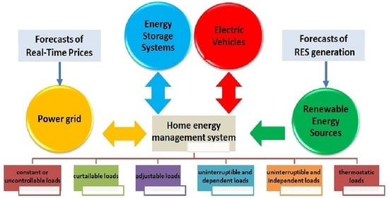
As it is clear from the provided literature review, several works deal with the smart home energy optimization problem from many perspectives, the majority of which cover all the aspects of the studied problem partially. This work is based on the development of an optimization approach, namely, a MILP model, for optimal smart home energy management, including all types of smart loads (uncontrollable loads, curtailable, adjustable, uninterruptible and independent loads, uninterruptible and dependent loads, and thermostatic ones), RES, in the form of wind and photovoltaic power contribution, ESS, EV, and energy exchanges with the power grid. This work comprises an extension of the work presented in [25], on the grounds that it incorporates the following:

i.

A forecasting approach is proposed combining clustering and neural network. The critical variables that affect the prosumer’s expenses are electricity prices. Photovoltaics (PV) generation and wind turbine (WT) generation are employed in the forecasting process. The clustering part of the forecasting model is utilized for the optimal selection of historical values of the target variable;

ii.

A peak load constraint has been added in the mathematical formulation, exerting significant influence on the decision making;

iii.

A more detailed temporal granularity has been employed, namely, 15 min time step instead of an hourly one in [25];

iv.

The case studies executed include both summer and winter days, providing the ability to capture the seasonal fluctuation in terms of RES generation and the operation of thermostatic loads.

Thus, the salient feature of the present work that is among few works in the literature integrates scheduling of both supply and demand sides, including the flexibility providers and all types of smart loads.

The developed modeling framework has been assessed on an illustrative case study, including a summer and a winter day, to demonstrate its applicability and effectiveness. It aims at capturing the time dynamics and interdependencies among the load scheduling, the flexibility provided by EVs and ESSs, the renewable energy contribution, and the interaction with the power grid. This systematic approach enhances decentralized energy generation, converting passive consumers into active prosumers, and is characterized by significant flexibility on the grounds that it can be easily adapted for large-scale case studies at a neighborhood and/or an urban level.

The main decision variables to be determined by the optimization approach are (i) RES generation scheduling (allocation of the energy generation and interactions with the grid), (ii) optimal load dispatch of the home’s smart appliances, and (iii) optimal operation of flexibility providers (ESS and EV).

Following the Introduction section, the work’s structure has the following form: Section 2 presents the mathematical model formulation of the underlying problem and is followed by Section 3, explaining the modeling approach of the forecasting processes whose outputs provide some of the required inputs to the optimization model. The assumptions and the input data of the employed case studies are described in Section 4, and Section 5 provides a detailed discussion of the model solution outputs. Last but not least, Section 6 summarizes the key findings of the work.

2. Mathematical Model Formulation

Figure 1 illustrates the graphical flowchart of the developed optimization approach. The smart home consists of different types of appliances classified into six load types according to the following: (i) constant or uncontrollable loads, (ii) curtailable loads, (iii) adjustable loads, (iv) uninterruptible and independent loads, (v) uninterruptible and dependent loads, and (vi) thermostatic loads (air-conditioning, refrigerator, and water heater). In addition, flexibility providers are modeled, including an ESS and an EV, as well as RES generation, enabling the energy exchanges with the power grid. The problem under consideration is formally defined according to the following:

2.1. Objective Function

The objective function refers to the minimization of the smart home’s total net daily cost, namely, the total daily cost for electricity purchases from the grid minus the total daily profits from electricity sales to the grid, as stated by Equation (1).

$$Min TC={{\displaystyle \sum }}_t\left(C_t^{buy}·P_t^{grid}-R_t^{sell}·P_t^{sell}\right)$$

(1)

2.2. Demand Balance

The demand balance states that the total electricity supply from the power grid, plus the RES-based electricity generation, plus the ESS and EV discharging directed for the household’s energy requirements must meet the dynamic load of all smart appliances in each time period, as presented in Equation (2).

$$P_t^{Grid,home}+P_t^{RES,home}+P_t^{ESS,home}+P_t^{EV,home}={\displaystyle \sum }_w{L}_{w,t},\forall t$$

(2)

2.3. Energy Storage Modeling

As stated by Equation (3), the amount of energy stored in the ESS in each time period equals the corresponding stored amount of the previous time period, plus the ESS charging power, taking into account the ESS charging efficiency, minus the ESS discharging power

$$B_t^{ESS}=B_{t-1}^{ESS}+F^{CH,ESS}·P_t^{ESS,char}-P_t^{ESS,disc} \forall t$$

(3)

The state-of-energy in the ESS must also be bounded between specific limits, as set by Constraint (4).

$$B^{ESS,min}\le B_t^{ESS}\le B^{ESS,max} \forall t$$

(4)

The amount of ESS charging power includes power originating from the power grid, the electric vehicle, and on-site renewable energy generation, based on Equation (5).

$$P_t^{ESS,char}=P_t^{Grid,ESS}+P_t^{EV,ESS}+P_t^{RES,ESS} \forall t$$

(5)

In the same context, the amount of net ESS discharging power, taking into account the battery’s discharging efficiency, can be directed to household energy requirements and EV charging, as defined by Equations (6) and (7).

$$P_t^{ESS,used}=F^{DC,ESS}·P_t^{ESS,disc} \forall t$$

(6)

$$P_t^{ESS,used}=P_t^{ESS,home}+P_t^{ESS,EV} \forall t$$

(7)

The charging and discharging power are bounded by maximum rates (Constraints (8) and (9)) and the available capacity space in the battery in each time period (Constraints (10) and (11)).

$$P_t^{ESS,char}\le CH{R}^{ESS}·x_t^{ESS,char} \forall t$$

(8)

$$P_t^{ESS,disc}\le DC{R}^{ESS}·x_t^{ESS,disc} \forall t$$

(9)

$$P_t^{ESS,char}\le B^{ESS,max}-B_{t-1}^{ESS} \forall t$$

(10)

$$P_t^{ESS,disc}\le B_{t-1}^{ESS}-B^{ESS,min} \forall t$$

(11)

Finally, charging and discharging decisions cannot be taken simultaneously (Constraint (12)).

$$x_t^{ESS,char}+x_t^{ESS,disc}\le 1 \forall t$$

(12)

2.4. Electric Vehicles Modeling

Similar to the corresponding Equation (3) for the ESS, Equation (13) states that the amount of energy stored in the EV in each time period ($B_t^{EV}$) equals the corresponding amount of the previous time period ($B_{t-1}^{EV}$), plus the EV charging power ($P_t^{EV,char}$), taking into account the EV battery’s charging efficiency ($F^{CH,EV}$), and minus the gross EV discharging power ($P_t^{EV,disc}$), according to Equation (3).

$$B_t^{EV}=B_{t-1}^{EV}+F^{CH,EV}·P_t^{EV,char}-P_t^{EV,disc} \forall t$$

(13)

The state-of-energy in the EV battery ($B_t^{EV}$) has corresponding upper ($B^{EV,max}$) and lower limits ($B^{EV,min}$), as set by Constraint (14).

$$B^{EV,min}\le B_t^{EV}\le B^{EV,max} \forall t$$

(14)

According to Equation (15), the amount of EV charging power ($P_t^{EV,char}$) equals the charging power from the power grid ($P_t^{Grid,EV}$), the ESS ($P_t^{ESS,EV}$), and the component of RES generation directed to the EV ($P_t^{RES,EV}$).

$$P_t^{EV,char}=P_t^{Grid,EV}+P_t^{ESS,EV}+P_t^{RES,EV} \forall t$$

(15)

Based on Equation (16), the amount of EV net discharging power ($P_t^{EV,used}$) equals the EV gross discharging power ($P_t^{EV,disc}$), multiplied by the EV battery’s discharging efficiency ($F^{DC,EV}$). Equation (17) determines that this amount ($P_t^{EV,used}$) can be directed to cover the household’s requirements ($P_t^{EV,home}$), and it can contribute to the ESS charging ($P_t^{EV,ESS}$).

$$P_t^{EV,used}=F^{DC,EV}·P_t^{EV,disc} \forall t$$

(16)

$$P_t^{EV,used}=P_t^{EV,home}+P_t^{EV,ESS} \forall t$$

(17)

The EV charging ($P_t^{EV,char}$) and discharging ($P_t^{EV,disc}$) power are bounded by maximum rates (Constraints (18) and (19)), subject to the decisions for charging ($x_t^{EV,char}$) and discharging ($x_t^{EV,disc}$), correspondingly, or not. They are also bounded by the available capacity space in the EV battery in each time period (Constraints (20) and (21)).

$$P_t^{EV,char}\le CH{R}^{EV}·x_t^{EV,char} \forall t$$

(18)

$$P_t^{EV,disc}\le DC{R}^{EV}·x_t^{EV,disc} \forall t$$

(19)

$$P_t^{EV,char}\le B^{EV,max}-B_{t-1}^{EV} \forall t$$

(20)

$$P_t^{EV,disc}\le B_{t-1}^{EV}-B^{EV,min} \forall t$$

(21)

Constraint (22) guarantees that the charging ($x_t^{EV,char}$) and discharging ($x_t^{EV,disc}$) decisions cannot be implemented simultaneously during the same time period.

$$x_t^{EV,char}+x_t^{EV,disc}\le 1 \forall t$$

(22)

Comparing to the ESS modeling, two additional constraints guarantee that when the EV is out of home ($x_t^{OFF}=1$), it is not available for charging and discharging decisions (Constraints (23) and (24)).

$$x_t^{EV,char}\le 1-x_t^{OFF} \forall t$$

(23)

$$x_t^{EV,disc}\le 1-x_t^{OFF} \forall t$$

(24)

2.5. Renewable Generation and Interaction with the Grid

The amount of renewable electricity generation ($P_t^{RES,prod}$) can be either utilized locally ($P_t^{RES,used}$) or sold back to the grid ($P_t^{RES,sell}$) (Equation (25)).

$$P_t^{RES,prod}=P_t^{RES,used}+P_t^{RES,sell} \forall t$$

(25)

The amount of power that is locally used ($P_t^{RES,used}$) can be directed to ESS ($P_t^{RES,ESS}$), EV battery ($P_t^{RES,EV}$), and home energy consumption ($P_t^{RES,home}$) (Equation (26)).

$$P_t^{RES,used}=P_t^{RES,ESS}+P_t^{RES,EV}+P_t^{RES,home} \forall t$$

(26)

The total amount of energy that is sold to the grid ($P_t^{sell}$) is the corresponding part of the RES-based electricity generation ($P_t^{RES,sell}$) (Equation (27)).

$$P_t^{sell}=P_t^{RES,sell} \forall t$$

(27)

The total amount of power supply from the grid ($P_t^{Grid}$) is split into three parts, namely, from grid to ESS ($P_t^{Grid,ESS}$), EV ($P_t^{Grid,EV}$), and home energy ($P_t^{Grid,home}$) (Equation (28)).

$$P_t^{Grid}=P_t^{Grid,ESS}+P_t^{Grid,EV}+P_t^{Grid,home} \forall t$$

(28)

The energy exchanges with the grid ($P_t^{Grid}$ and $P_t^{sell}$) are bounded by a maximum amount in each time period ($TB$ and $TS$), subject to the decision for electricity purchases from or sales to the grid ($x_t^{Grid}$) (Constraints (29) and (30)).

$$P_t^{Grid}\le TB·x_t^{Grid} \forall t$$

(29)

$$P_t^{sell}\le TS·\left(1-x_t^{Grid}\right) \forall t$$

(30)

2.6. Load Types

Six types of loads $w\in W$ are modeled. These concern (i) constant or uncontrollable loads, (ii) curtailable loads, (iii) adjustable loads, (iv) uninterruptible and independent loads, (v) uninterruptible and dependent loads, and (vi) thermostatic loads (air-conditioning, refrigerator, and water heater).

2.6.1. Constant or Uncontrollable Loads

The first load type refers to constant or uncontrollable load $w\in W^{co}$, whose operation is deterministic and continuous and cannot be interrupted, adjusted, and/or curtailed (Equation (31)).

$$L_{w,t}={\tilde{L}}_{w,t}·\forall w\in W^{co},t$$

(31)

2.6.2. Curtailable Loads

The second type of loads concerns curtailable load $w\in W^{cu}$, which can be totally curtailed for certain time periods (Equation (32)). Operation and curtailment decisions cannot be taken simultaneously (Constraint (33)). If it is operational ($x_{w,t}^{oper}=1$), it operates with its full load (Constraint (34)), while in case of curtailment ($x_{w,t}^{crt}=1$), its power output is zero (Equation (35)).

$${\displaystyle \sum }_t{x}_{w,t}^{crt}\le C{N}_w \forall w\in W^{cu}$$

(32)

$$x_{w,t}^{oper}+x_{w,t}^{crt}\le 1 \forall w\in W^{cu},t$$

(33)

$$L_{w,t}={\tilde{L}}_{w,t}·x_{w,t}^{oper} \forall w\in W^{cu},t$$

(34)

$$c{r}_{w,t}={\tilde{L}}_{w,t}·x_{w,t}^{crt} \forall w\in W^{cu},t$$

(35)

2.6.3. Adjustable Loads

The third type of load concerns the adjustable load $w\in W^{adj}$ whose power demand can be adjusted/modified (Equations (36) and (37)), subject to the decision for adjustment or not ($x_{w,t}^{adj}$), based on the comparison of the forecasted power price with an imposed price limit (Constraints (38)).

$$L_{w,t}={\tilde{L}}_{w,t}·\left(1-x_{w,t}^{adj}\right)+{\tilde{L}}_{w,t}^{adj}·x_{w,t}^{adj} \forall w\in W^{adj},t$$

(36)

$${\tilde{L}}_{w,t}^{adj}=C_1·{\tilde{L}}_{w,t} \forall w\in W^{adj},t$$

(37)

$$N·\left(P{R}_t-P{R}_{w,t}^{min}\right)\le x_{w,t}^{adj}\le N·\left(P{R}_t-P{R}_{w,t}^{min}\right)+1 \forall w\in W^{adj},t$$

(38)

2.6.4. Uninterruptible and Independent Loads

The fourth type of load has to do with uninterruptible and independent loads $w\in W^{und}$. Once they start-up, at least a certain time before the end of the scheduling period and within the desired time limits $\left[T_w^{on},T_w^{off}\right]$ (Equation (39)), it remains operational without interruptions and adjustments until the end of its operational duration (Equations (40) and (41)).

$${\displaystyle \sum }_{t=T_w^{on}}^{T_w^{off}-Du{r}_w+1}{x}_{w,t}^{st}=1 \forall w\in W^{und}$$

(39)

$$x_{w,t}^{oper}={\displaystyle \sum }_{t^{\prime }=t-Du{r}_w+1}^t{x}_{w,t^{\prime }}^{st} \forall w\in W^{und},t\in \left[T_w^{on},T_w^{off}\right]$$

(40)

$${\displaystyle \sum }_t{x}_{w,t}^{oper}=Du{r}_w \forall w\in W^{und}$$

(41)

A logical constraint correlating the start-up, shut-down, and operating decisions are defined by Equation (42). Its total power consumption per time period is provided by Equation (43), subject to the decision of its operation or not.

$$x_{w,t}^{oper}-x_{w,t-1}^{oper}=x_{w,t}^{st}-x_{w,t}^{sd} \forall w\in W^{und},t$$

(42)

$$L_{w,t}={\tilde{L}}_{w,t}·x_{w,t}^{oper} \forall w\in W^{und},t$$

(43)

2.6.5. Uninterruptible and Dependent Loads

The fifth type of loads covers the uninterruptible and dependent among the loads $w\in W^{ud}$. All the constraints describing the operation of uninterruptible and independent loads $w\in W^{und}$ (Equations (39)–(43)) are also active (here Equations (44)–(48)), and an additional constraint (uninterruptible–dependent–consecutive) is introduced to state that the operation of one appliance (e.g., washing machine) has to be completed in order for a consecutive task (e.g., dryer) to be able to start-up (Equation (49)). In addition, there is also another kind of dependence, stating that the operation of one appliance (e.g., printer) is subject to the concurrent operation of another appliance (e.g., desktop), as stated by Constraint (50).

$${\displaystyle \sum }_{t=T_w^{on}}^{T_w^{off}-Du{r}_w+1}{x}_{w,t}^{st}=1 \forall w\in W^{ud}$$

(44)

$$x_{w,t}^{oper}={\displaystyle \sum }_{t^{\prime }=t-Du{r}_w+1}^t{x}_{w,t^{\prime }}^{st} \forall w\in W^{ud},t\in \left[T_w^{on},T_w^{off}\right]$$

(45)

$$x_{w,t}^{oper}-x_{w,t-1}^{oper}=x_{w,t}^{st}-x_{w,t}^{sd} \forall w\in W^{ud},t$$

(46)

$${\displaystyle \sum }_t{x}_{w,t}^{oper}=Du{r}_w \forall w\in W^{ud}$$

(47)

$$L_{w,t}={\tilde{L}}_{w,t}·x_{w,t}^{oper} \forall w\in W^{ud},t$$

(48)

$$x_{w,t}^{st}={\displaystyle \sum }_{t^{\prime }\le t}^t{x}_{w,t^{\prime }}^{sd} \forall w\in W^{ud-cons},t$$

(49)

$$x_{w,t}^{oper}\le x_{w^{\prime },t}^{oper} \forall \left(w,w^{\prime }\right)\in W^{ud-cons},t$$

(50)

2.6.6. Thermostatic Loads

The sixth type of loads refers to thermostatic loads, including three thermal appliances such as a heater/air conditioner, a refrigerator, and a water heater. The modeling of this type of load follows the same approach as presented in [7].

Heater/Air Conditioner

Constraints (51)–(54) model the air conditioner’s operation in both the heating and cooling modes. According to Constraint (51), the home inside temperature ($T_t^{AC,in}$) is a function of the corresponding temperature in the previous time period ($T_{t-1}^{AC,in}$), plus the thermal conductivity of home to outside $g·\left(T_t^{out}-T_t^{AC,in}\right)$, and the cooling and heating rate ($g^{AC}$ and $g^H$), subject to the relevant activation or not ($x_t^{AC}$ and $x_t^H$). Constraint (52) sets the lower and upper limits of the home inside temperature, and Constraint (53) states that the air conditioner can operate to at most one mode (heating or cooling) in each time period. Finally, Equation (54) determines the final load of the air conditioner in each time period.

$$T_t^{AC,in}=T_{t-1}^{AC,in}+g·\left(T_t^{out}-T_t^{AC,in}\right)-g^{AC}·x_t^{AC}+g^H·x_t^H \forall t$$

(51)

$$T^{AC,min}\le T_t^{AC,in}\le T^{AC,max} \forall t$$

(52)

$$x_t^{AC}+x_t^H\le 1 \forall t$$

(53)

$$L_{w,t}={\tilde{L}}_{w,t}·\left(x_t^{AC}+x_t^H\right) \forall w\in W^{AC},t$$

(54)

Refrigerator

According to Constraint (55), the home inside temperature ($T_t^{fr,in}$) is a function of the corresponding temperature in the previous time period ($T_{t-1}^{FR,in}$), plus the warming rate of the fridge $\left(g^{fr,h}\right)$, minus its cooling rate ($g^{fr,c}$), subject to the refrigerator’s operation or not ($x_t^{fr}$). Constraint (56) sets the lower and upper limits of the fridge inside temperature, and Equation (57) determines the refrigerator’s final load in each time period.

$$T_t^{fr,in}=T_{t-1}^{FR,in}+g^{fr,h}-g^{fr,c}·x_t^{fr} \forall t$$

(55)

$$T^{fr,min}\le T_t^{fr,in}\le T^{fr,max} \forall t$$

(56)

$$L_{w,t}={\tilde{L}}_{w,t}·x_t^{fr} \forall w\in W^{fr},t$$

(57)

Water Heater

Constraints (58)–(60) describe the same constraints for the water heater as those of the refrigerator.

$$T_t^{wh,in}=T_{t-1}^{wh,in}+g^{wh,h}·x_t^{wh}-g^{wh,c} \forall t$$

(58)

$$T^{wh,min}\le T_t^{wh,in}\le T^{wh,max} \forall t$$

(59)

$$L_{w,t}={\tilde{L}}_{w,t}·x_t^{wh} \forall w\in W^{wh},t$$

(60)

2.7. Peak Load

Finally, Constraint (61) defines that the total load in each time period (${\displaystyle \sum }_w{L}_{w,t}$) must not exceed an imposed peak value ($PL$).

$${\displaystyle \sum }_w{L}_{w,t}\le PL \forall t$$

(61)

The overall problem is formulated as a MILP model aiming at minimizing the household’s total net daily cost (1), and subject to constraints (2)–(61).

3. Forecasting Processes

The scope of forecasting processes is the optimal strategic utilization of the prosumer resources in order to reach out in minimal energy costs. In this paper, a method of selecting the proposer inputs for the forecasting model is proposed. The prosumer model is applied to two test cases, namely, the summer day and the winter day. Figure 2 shows the connection of the forecasting processes and the prosumer model. The latter receives inputs the forecasts and is executed every time step. The proposed forecasting model refers to a combination of unsupervised and supervised machine learning algorithms. The unsupervised machine learning part corresponds to clustering. The K-medoids algorithm is employed for proper selection of the training inputs [26]. The supervised part refers to the Elman neural network (ENN) [27]. The role of ENN is to perform the forecasts of the three variables. Figure 3 displays the flowchart of the hybrid forecasting model. The same model is used for all variables. The difference lies on the types and number of inputs of the ENN. Let $x_n^{\left(q\right)}, q=1,2,\dots ,Q, n=1,2,\dots ,N$ be an input pattern of the ENN, where $x_n^q$ denotes the $n$th component of the $q$ feature vector $x^{\left(q\right)}=\left[x_1^{\left(q\right)},\dots ,x_N^{\left(q\right)}\right].$ The data are normalized in the [0, 1] range by dividing each element of $x^{\left(q\right)}$ with the maximum value among the $Q$ values. The normalization aids at the better exploitation of clustering results. In the clustering procedure, the scope is to group together patterns with similar characteristics. In the case of Real-Time Prices (RTP) and generation, the similarity lies on the similarity of the time series shapes. The pattern corresponds to the time series that cover a 24 h period. K-medoids is applied for the proper selection of historical data that will be used for the training of the ENN. Let $d$ be the target day of forecasting, i.e., either the summer or winter day. The training input selection process is composed by the following steps:

• Step#1: Conduct a correlation analysis between the current time instance (i.e., 15 min) $h$ of day $d$ with all previous hours from the start date of the available dataset. For example, Figure 3 presents the Pearson correlation coefficient curves for the summer and winter days up to 196 h in the past [28]. It can be noticed that day $d$ is more corelated with day $d-1$.
• Step#2: Apply K-medoids for $k$ number of clusters to all days up to $d-1$.
• Step#3: Locate the cluster that day $d-1$ belongs to.
• Step#4: Calculate the Euclidean distances between all days in the same cluster of day $d-1$ and day $d-1$.
• Step#5: Sort the according distances in ascending order.
• Step#6: Selected $m$ days on the top of the order and train ENN using this set.

The above process leads to the selection of the most similar days to day $d$, which refers to the target day. According to Figure 3, external variables are utilized as inputs. For the RTP forecasting process, the RTPs of the two test days are predicted using only historical values. More specifically, it is regarded that the prosumer purchases electricity from a retailer. The RTP is the forecasted system marginal price (SMP) increased by 65%. This increase is necessary for the retailer to cover its operational expenses and witness profit. RES generation includes photovoltaics (PV) and small wind turbines (WT). Let $RTP\left(h+1\right), PV\left(h+1\right)$, and $WT\left(h+1\right)$ be the RTP, PV generation, and WT generation of time instance $h+1,$ respectively. These variables refer to the outputs of the forecasting model.

Table 1. Outputs and inputs of the forecasting model.

Outputs	Inputs
$RTP\left(h+1\right)$	$RTP\left(h-1\right)$	$RTP\left(h\right)$	-	-
$PV\left(h+1\right)$	$PV\left(h-1\right)$	$PV\left(h\right)$	$Temp\left(h\right)$	$CSI\left(d\right)$
$WT\left(h+1\right)$	$WT\left(h-1\right)$	$WT\left(h\right)$	$Temp\left(h\right)$	$WS\left(d\right)$

presents the outputs and the inputs of the model. The forecasts of PV and WT generations include external variables, namely, mean daily temperature of day, $Temp\left(d\right)$, clearness sky index of day $d, CSI\left(d\right),$ and mean daily wind speed of day $d, WS\left(d\right).$ The selected time lags $h$ and $h-1$ are selected via correlation analysis. Figure 4 presents the correlation coefficient curves for the two test days.

K-medoids is a partitional clustering algorithm. Prior to its execution, the most significant parameters that needs to be defined are the number of training epochs, the objective function threshold improvement, and the selection of initial centroids method. These have been selected with a trial-and-error procedure. Specifically, the number of epochs is set to 500, the threshold to 10⁻⁶ and the centroids are initialized randomly. Let $k=1,2,\dots ,K$ be the indicator denoting the number of clusters, and $K$ is the number of clusters. Each cluster is presented by the medoid, which is the median of all patterns of the cluster. Let $m^{\left(k\right)}$ be the medoid of the $k$-th cluster. Through a number of iterations, K-medoids aims at minimizing the sum of squared errors (SSE) between pattern $x^{\left(q\right)}$ and each medoid of the clusters:

$$\mathrm{SSE}={{\displaystyle \sum }}_{q=1}^Q{{\displaystyle \sum }}_{k=1}^K{d}_E(x^{\left(q\right)},m^{\left(k\right)})$$

(62)

For ENN, the following structure is selected: one hidden layer, resilient back-propagation training algorithm, tangent sigmoid activation function for the neurons of the hidden and output layers, number of epochs 500, and objective function threshold improvement 10⁻⁶ [29]. The training error refers to mean absolute percentage error (MAPE) [30].

In order to fully evaluate the performance of ENN, a comparison takes place between ENN and an auto-regressive integrated moving average (ARIMA) model [31]. Prior to its implementation, the order of the model needs to be defined. Let $y\left(h\right)$ be the value of variable $y$ in next hour $h.$ The ARIMA model treats future values of the variable as a linear combination of historical values. ARIMA is composed of the sum of auto-regressive (AR) and moving average (MA) components. The AR(p) component is obtained by the following expression:

$$y\left(h\right)={\phi }_{1}y\left(h-1\right)+{\phi }_{2}y\left(h-2\right)+\cdots +{\phi }_{p}y\left(h-p\right)+c+{\epsilon }_p$$

(63)

where p is the order of the model, ${\phi }_1,{\phi }_2,\dots .,{\phi }_p$ are the factors of the AR components, $c$ is a constant, and ${\epsilon }_p$ is white noise. The moving average (MA) components consider part errors. The MA(q) component is obtained by the following expression:

$$y\left(h\right)={\theta }_1\epsilon \left(h-1\right)+{\theta }_2\epsilon \left(h-2\right)+\cdots +{\theta }_p\epsilon \left(h-q\right)+c+{\epsilon }_q$$

(64)

where q is the order of the model, ${\theta }_1,{\theta }_2,\dots .,{\theta }_q$ are the factors of the AR components, $c$ is a constant, and ${\epsilon }_q$ is white noise. By combining Equations (63) and (64), the ARIMA model expression is obtained:

$$y\left(h\right)={\phi }_{1}y\left(h-1\right)+{\phi }_{2}y\left(h-2\right)+\cdots +{\phi }_{p}y\left(h-p\right)+{\theta }_1\epsilon \left(h-1\right)+{\theta }_2\epsilon \left(h-2\right)+\cdots +{\theta }_p\epsilon \left(h-q\right)+c+{\epsilon }_h$$

(65)

where ${\epsilon }_h$ is white noise. The model is represented as ARIMA($p$,$d$,$q$), where $d$ is the number of differentiation needed for the time series to become stationary. In order to select the order of the model, the sample auto-correlation function (SAF) and sample partial auto-correlation function (SPAF) are checked. Figure 5 presents the SPAF for the RTP, and Figure 6, Figure 7, Figure 8 and Figure 9 present the SAF and SPAF of PV and WT generation, respectively.

By checking Figure 4a and Figure 5, the RTP series presents a correlation with high order lags. This is not the case for PV and WT generation. In order to select the order of the model, Akaike’s information criterion (AIC) and Bayesian information criterion (BIC) are considered. They are given by the following equations, respectively:

$$A\left.IC=-2\log \left(L\right)+2(p+q+k+1\right)$$

(66)

$$\left.BIC=\mathrm{AIC}+\left[\log \left(T\right)-2\right](p+q+k+1\right)$$

(67)

where $L$ is the log-likelihood estimate, $k$ is the number of independent variables used, and $T$ is the number of observations. Thus, a series of different structures are examined. Different combiations of $p$ and $q$ are take into account.

Table 2. Akaike’s information criterion (AIC) and Bayesian information criterion (BIC) scores for auto-regressive integrated moving average (ARIMA)($p,0,q)$ models for RTP forecasting of summer day.

AR($\mathit{p}$)	MA($\mathit{q}$)	$\mathit{A}\mathit{I}\mathit{C}$	$\mathit{B}\mathit{I}\mathit{C}$	AR($\mathit{p}$)	MA($\mathit{q}$)	$\mathit{A}\mathit{I}\mathit{C}$	$\mathit{B}\mathit{I}\mathit{C}$
1	1	1783.71	1791.53	4	1	1711.98	1727.61
1	2	1495.86	1506.28	4	2	1776.17	1794.40
1	3	1484.57	1497.59	4	3	1467.93	1488.77
1	4	1773.85	1789.48	4	4	1449.12	1472.57
1	5	1773.62	1791.86	4	5	1762.45	1788.50
1	6	1423.30	1444.14	4	6	1758.30	1786.95
2	1	1770.98	1781.40	5	1	1532.06	1550.30
2	2	1483.74	1496.77	5	2	1428.94	1449.78
2	3	1762.63	1778.26	5	3	1411.79	1435.24
2	4	1756.87	1775.11	5	4	1761.13	1787.18
2	5	1472.56	1493.41	5	5	1755.02	1783.68
2	6	1437.49	1460.93	5	6	1395.41	1426.68
3	1	1772.43	1785.46	6	1	1442.48	1463.33
3	2	1487.91	1503.54	6	2	1417.58	1441.03
3	3	1758.89	1777.12	6	3	1423.03	1449.08
3	4	1758.33	1779.17	6	4	1209.52	1238.18
3	5	1755.47	1778.92	6	5	1026.48	1057.75
3	6	1741.28	1767.33	6	6	1033.58	1067.45

and

Table 3. AIC ad BIC scores for ARIMA($p,1,q)$ models for RTP forecasting of summer day.

AR($\mathit{p}$)	MA($\mathit{q}$)	$\mathit{A}\mathit{I}\mathit{C}$	$\mathit{B}\mathit{I}\mathit{C}$	AR($\mathit{p}$)	MA($\mathit{q}$)	$\mathit{A}\mathit{I}\mathit{C}$	$\mathit{B}\mathit{I}\mathit{C}$
1	1	1499.43	1507.24	4	1	1464.45	1480.08
1	2	1485.51	1495.93	4	2	1408.71	1426.94
1	3	1486.58	1499.61	4	3	1476.94	1497.79
1	4	1469.11	1484.74	4	4	1483.42	1506.86
1	5	1432.20	1450.43	4	5	967.55	993.61
1	6	1426.58	1447.42	4	6	896.01	924.66
2	1	1485.33	1495.75	5	1	1431.93	1450.17
2	2	1487.32	1500.35	5	2	1364.40	1385.24
2	3	1486.68	1502.31	5	3	1360.75	1384.20
2	4	1447.93	1466.16	5	4	1027.54	1053.59
2	5	1429.74	1450.58	5	5	944.80	973.45
2	6	1428.43	1451.88	5	6	878.25	909.51
3	1	1487.33	1500.36	6	1	1421.26	1442.11
3	2	1488.19	1503.82	6	2	1309.53	1332.97
3	3	1425.55	1443.79	6	3	1378.04	1404.09
3	4	1486.78	1507.63	6	4	1028.35	1057.01
3	5	1401.30	1424.74	6	5	867.36	898.63
3	6	1400.72	1426.77	6	6	897.21	931.08

present the scores of the various examined models of ARIMA($p,0,q)$ and ARIMA($p,1,q)$ for RTP forecasting, respectively. The tables refer to the summer day. The scores are calculated using the same training set that the ENN has used. The selected structure should lead to lower values to AIC and BIC. It can be observed that, in general, ARIMA($p,1,q)$ results in better scores compared to ARIMA($p,1,q).$ The best scores are met at the ARIMA($5,1,6)$ model.

Table 4. AIC ad BIC scores for ARIMA($p,0,q)$ models for PV forecasting of summer day.

AR($\mathit{p}$)	MA($\mathit{q}$)	$\mathit{A}\mathit{I}\mathit{C}$	$\mathit{B}\mathit{I}\mathit{C}$	AR($\mathit{p}$)	MA($\mathit{q}$)	$\mathit{A}\mathit{I}\mathit{C}$	$\mathit{B}\mathit{I}\mathit{C}$
1	1	56,639.20	56,647.02	4	1	55,838.63	55,854.26
1	2	55,447.22	55,457.64	4	2	54,782.52	54,800.75
1	3	54,917.67	54,930.7	4	3	54,781.87	54,802.71
1	4	54,784.64	54,800.27	4	4	54,781.21	54,804.66
1	5	55,059.40	55,077.63	4	5	54,779.63	54,805.68
1	6	54,783.48	54,804.32	4	6	54,780.01	54,808.66
2	1	56,206.77	56,217.19	5	1	55,737.22	55,755.46
2	2	54,818.10	54,831.12	5	2	54,782.01	54,802.85
2	3	54,780.50	54,796.13	5	3	54,776.52	54,799.97
2	4	54,777.55	54,795.79	5	4	54,778.39	54,804.44
2	5	54,779.32	54,800.16	5	5	54,799.74	54,828.4
2	6	54,777.95	54,801.39	5	6	54,781.95	54,813.21
3	1	56,006.35	56,019.37	6	1	55,653.02	55,673.86
3	2	54,783.35	54,798.98	6	2	54,783.53	54,806.98
3	3	54,784.44	54,802.68	6	3	54,778.37	54,804.42
3	4	54,779.53	54,800.37	6	4	54,784.55	54,813.21
3	5	54,779.56	54,803.01	6	5	54,782.09	54,813.35
3	6	54,786.07	54,812.13	6	6	54,796.78	54,830.64

and

Table 5. AIC ad BIC scores for ARIMA($p,1,q)$ models for PV forecasting of summer day.

AR($\mathit{p}$)	MA($\mathit{q}$)	$\mathit{A}\mathit{I}\mathit{C}$	$\mathit{B}\mathit{I}\mathit{C}$	AR($\mathit{p}$)	MA($\mathit{q}$)	$\mathit{A}\mathit{I}\mathit{C}$	$\mathit{B}\mathit{I}\mathit{C}$
1	1	56,312.77	56,320.59	4	1	56,246.17	56,261.81
1	2	56,244.92	56,255.34	4	2	56,240.49	56,258.72
1	3	56,245.62	56,258.64	4	3	54,648.27	54,669.11
1	4	56,246.43	56,262.06	4	4	54,617.65	54,641.10
1	5	56,248.06	56,266.30	4	5	54,617.43	54,643.48
1	6	56,249.98	56,270.82	4	6	56,230.71	56,259.37
2	1	56,244.12	56,254.54	5	1	56,248.02	56,266.26
2	2	56,245.81	56,258.84	5	2	56,242.47	56,263.31
2	3	56,242.91	56,258.54	5	3	54,620.19	54,643.64
2	4	56,240.46	56,258.69	5	4	56,224.39	56,250.44
2	5	56,242.46	56,263.3	5	5	56,241.58	56,270.23
2	6	56,244.27	56,267.71	5	6	56,247.98	56,279.24
3	1	56,245.74	56,258.76	6	1	56,249.96	56,270.80
3	2	56,238.75	56,254.39	6	2	56,243.98	56,267.43
3	3	56,240.49	56,258.73	6	4	56,244.55	56,270.60
3	4	56,242.46	56,263.30	6	5	56,236.25	56,264.91
3	5	56,244.46	56,267.9	6	5	56,231.14	56,262.41
3	6	56,239.35	56,265.41	6	6	56,249.98	56,283.85

show the scores of ARIMA($p,0,q)$ and ARIMA($p,1,q)$ for PV generation forecasting, respectively. Finally,

Table 6. AIC ad BIC scores for ARIMA($p,0,q)$ models for WT forecasting of summer day.

AR($\mathit{p}$)	MA($\mathit{q}$)	$\mathit{A}\mathit{I}\mathit{C}$	$\mathit{B}\mathit{I}\mathit{C}$	AR($\mathit{p}$)	MA($\mathit{q}$)	$\mathit{A}\mathit{I}\mathit{C}$	$\mathit{B}\mathit{I}\mathit{C}$
1	1	206,917.16	206,924.98	4	1	206,661.55	206,685.00
1	2	206,691.43	206,701.85	4	2	206,643.59	206,669.64
1	3	206,693.35	206,706.37	4	3	206,706.12	206,721.75
1	4	206,669.42	206,685.05	4	4	206,670.98	206,689.22
1	5	206,670.62	206,688.85	4	5	206,661.12	206,681.96
1	6	206,665.06	206,685.90	4	6	206,674.88	206,698.33
2	1	206,758.05	206,768.47	5	1	206,676.34	206,702.39
2	2	206,693.32	206,706.34	5	2	206,665.26	206,693.91
2	3	206,680.36	206,695.99	5	3	206,705.35	206,723.59
2	4	206,674.23	206,692.47	5	4	206,669.29	206,690.13
2	5	206,663.98	206,684.82	5	5	206,654.99	206,678.43
2	6	206,657.26	206,680.71	5	6	206,637.58	206,663.63
3	1	206,736.14	206,749.17	6	1	206,650.51	206,679.17
3	2	206,669.09	206,684.72	6	2	206,646.07	206,677.33
3	3	206,673.15	206,691.38	6	3	206,703.54	206,724.38
3	4	206,664.94	206,685.78	6	4	206,698.04	206,721.49
3	5	206,917.16	206,924.98	6	5	206,654.45	206,680.50
3	6	206,691.43	206,701.85	6	6	206,692.57	206,721.22

and

Table 7. AIC ad BIC scores for ARIMA($p,1,q)$ models for WT forecasting of summer day.

AR($\mathit{p}$)	MA($\mathit{q}$)	$\mathit{A}\mathit{I}\mathit{C}$	$\mathit{B}\mathit{I}\mathit{C}$	AR($\mathit{p}$)	MA($\mathit{q}$)	$\mathit{A}\mathit{I}\mathit{C}$	$\mathit{B}\mathit{I}\mathit{C}$
1	1	207,085.79	207,093.61	4	1	206,943.04	206,958.68
1	2	207,000.29	207,010.71	4	2	206,812.29	206,830.52
1	3	206,911.81	206,924.83	4	3	206,801.26	206,822.10
1	4	206,908.82	206,924.45	4	4	206,766.28	206,789.73
1	5	206,900.16	206,918.39	4	5	206,728.25	206,754.30
1	6	206,901.75	206,922.59	4	6	206,727.43	206,756.09
2	1	207,005.10	207,015.52	5	1	206,943.06	206,961.29
2	2	207,012.26	207,025.29	5	2	206,806.24	206,827.08
2	3	206,869.32	206,884.95	5	3	206,724.08	206,747.52
2	4	206,804.53	206,822.77	5	4	206,745.76	206,771.81
2	5	206,786.37	206,807.21	5	5	206,722.39	206,751.04
2	6	206,778.07	206,801.52	5	6	206,711.20	206,742.46
3	1	206,941.38	206,954.41	6	1	206,938.73	206,959.57
3	2	206,867.59	206,883.22	6	2	206,804.62	206,828.06
3	3	206,869.13	206,887.37	6	3	206,714.76	206,740.81
3	4	206,817.14	206,837.98	6	4	206,714.79	206,743.45
3	5	206,726.52	206,749.96	6	5	206,715.22	206,746.48
3	6	206,715.97	206,742.03	6	6	206,718.79	206,752.66

show the scores of ARIMA($p,0,q)$ and ARIMA($p,1,q)$ for WT generation forecasting, respectively. For the PV generation, model ARIMA($3,0,4)$ is selected. For the WT generation, model ARIMA($5,0,6)$ is selected.

4. Case Study

The proposed optimization approach’s applicability has been assessed on an illustrative case study of a smart household. Two representative days, a typical winter and a summer day, have been selected with a 15-min time step.

Table 8. Key input data.

Electric Vehicles Modeling
$C_t^{buy}:$	Figure 5
$R_t^{sell}$:	0.0703 EUR/kW
$F^{CH,EV}:$	0.95
$F^{DC,EV}:$	0.95
$B^{EV,min}:$	12.5 kWh
$B^{EV,max}:$	50 kWh
$CH{R}^{EV}:$	11 kW
$DC{R}^{EV}:$	11 kW
Electricity Storage Modeling
$F^{CH,ESS}:$	0.95
$F^{DC,ESS}:$	0.95
$CH{R}^{ESS}:$	5 kW
$DC{R}^{ESS}:$	5 kW
$B^{ESS,max}:$	15 kWh
$B^{ESS,min}:$	3.75 kWh
Renewable Generation and Interaction with the Grid
$P_t^{RES,prod}:$	Figure 6
$TB$:	11 kW
$TS:$	11 kW

presents the mathematical model’s parameters’ values, categorizing them into EV, ESS, RES, and grid-related data. Figure 10 provides the RTP and the SMP forecasts of the two test days. The price for electricity exports to the grid is assumed to be constant during the whole day amounting to 0.0703 EUR/kW. Figure 11 depicts the forecasted PV and wind turbine availabilities during the summer and winter days, and Figure 12 shows the forecasted outside temperature on the summer and winter days, influencing the thermostatic loads’ operation.

Table 9. Household appliances’ specific characteristics.

Appliance	Type	Earliest Operating Time (15 min)	Latest Operating Time (15 min)	Duration (15 min)	Power (kW)
Dishwasher	Uninterruptible–Independent	00:00	23:45	4	1.4
Washing machine	Uninterruptible–Dependent–Consecutive	00:00	23:45	8	1.5
Dryer	Uninterruptible–Dependent–Consecutive	00:00	23:45	2	2.5
Refrigerator	Thermostatic	00:00	15:45	96	1.7
Oven	Uninterruptible–Dependent–Concurrent	06:00	10:45	2	2.4
Cooker hood	Uninterruptible–Dependent–Concurrent	08:00	10:45	2	0.2
Microwave	Uninterruptible–Independent	00:00	23:45	1	1.4
Water heater	Thermostatic	00:00	23:45	8	4.5
TV	Uninterruptible–Independent	06:00	23:45	20	0.1
Laptop	Uninterruptible–Independent	05:00	23:45	12	0.1
Desktop	Uninterruptible–Dependent–Concurrent	05:00	23:45	20	0.25
Printer	Uninterruptible–Dependent–Concurrent	05:00	23:45	2	0.011
Vacuum cleaner	Uninterruptible–Independent	00:00	11:45	4	1
Hair straightener	Uninterruptible–Dependent–Consecutive	09:00	15:45	2	0.055
Hairdryer	Uninterruptible–Dependent–Consecutive	09:00	15:45	2	1.8
Sensors	Uninterruptible–Independent	00:00	23:45	96	0.01
Radio player	Uninterruptible–Independent	22:00	23:45	4	0.2
AC/Heater	Thermostatic	00:00	15:45	48	1.45
Iron	Uninterruptible–Independent	00:00	11:45	2	2.5
Illumination	Adjustable	10:00	15:45	76	0.5
Occasional	Constant/Uncontrolalble	00:00	23:45	96	1.6
Curtailable	Curtailable	00:00	23:45	96	0.5

presents the home appliances’ specific characteristics, including the load type, duration, earliest starting operating time, and the latest operating time.

Figure 11 presents the graphical comparison between the ENN and ARIMA forecasts. Using the mean absolute range normalized error (MARNE) indicator of the forecasting accuracy is assessed [32].

Table 10. Mean absolute range normalized error (MARNE) values for the summer day.

Forecasting Model	RTP	PV	WT
ENN	4.32	3.69	5.94
ARIMA	5.14	9.22	7.55

and

Table 11. MARNE values for the winter day.

Forecasting Model	RTP	PV	WT
ENN	4.17	3.76	12.77
ARIMA	5.01	5.02	18.41

show the MARNEs of the models for the summer and winter days, respectively. It can be observed that the ENN results in lower errors in all the examined cases.

5. Results

This section provides the model outputs from the examined cases for the two representative days of summer and winter. The problem has been solved to global optimality using the ILOG CPLEX 12.6.0.0 solver incorporated in the General Algebraic Modeling System (GAMS) tool [33]. An integrality gap of 0% has been achieved in both cases.

5.1. Winter Day

Figure 13 presents the optimal demand allocation of the smart home appliances’ scheduling in each period of the winter day, satisfying the user’s time preferences simultaneously. The total daily load equals around 115.4 kWh, peak load amounts to 7.46 kW at 01:00, and the lowest load, being equal to 1.61 kW, is reported at 17:45 when only uncontrollable power loads and sensors are activated. Due to the electricity prices’ assumptions, almost 45% of the total daily load is activated during 0–8 h, followed by almost 29% in 8–16 h and 26% in 16–24 h. The constraints for uninterruptible and dependent among the loads are also satisfied; namely, the washing machine’s operation has to be completed in order for the task of the dryer to be able to start-up. Moreover, the model solution satisfies the other type of dependence, namely, the printer’s operation is subject to the desktop’s concurrent operation. The total daily net cost, namely, expenses for acquiring the grid’s electricity minus revenues from selling renewable electricity to the grid, for the smart home’s operational scheduling leads to small revenues of around EUR 6.60.

Figure 14 highlights the operational schedule of adjustable, curtailable, and thermostatic loads in each period of the winter day. The adjustment option of the adjustment load activates for 23 15-min time intervals (5.75 h in total), especially during 10–16 h. The curtailment load’s total curtailment load occurs during eight 15-min time intervals (2 h in total) of the day, especially between 19–20 h, when there is a combination of low RES availability and high electricity prices. Air-conditioning in the heating option (for 10.5 h), refrigerator (for 6.25 h), and water heater (for 5.5 h) are operational during several hours of the day to maintain the temperature settings.

Figure 15 depicts the optimal generation mix to satisfy home appliances’ power consumption on the winter day. As can be observed, grid power covers the largest part of the home loads during the majority of hours (51% in total at a daily level), and on-site RES generation meets almost 39% of the total at a daily level. It is also worth mentioning that the combined RES availability, based on the forecast conducted, is zero in 21–24 h. EV contributes around 6% of the whole load, covering the home’s consumption in the period 20:45–22:00 when the PV availability is zero, and wind is at relatively low or even zero levels. During the last seven time intervals, from 22:15 to 24:00, electricity imports the whole household load from the grid cover alone. Finally, ESS covers the remaining 4% in the energy contribution mix with relatively high percentages during several 15-min time intervals between 2–3 and 14–15 h.

Due to the existence of the constraint stating that the home cannot import and export energy simultaneously at the same period, renewable energy sales to the grid occur only during periods when the on-site infrastructure, ESS and EV, can cover the household load alone and/or in combination between them. Figure 16 represents the renewable energy balance highlighting the flows in each time period of the winter day. It can be seen that the majority of electricity exports to the grid occur when there is increased PV availability, namely, in the period 10–16 h.

Figure 17 depicts the state-of-energy in the ESS, including also the charging and discharging decision making. It is clear that the ESS is being charged only when there are electricity purchases from the grid, while its discharge occurs when there are RES electricity exports to the grid, and thus, ESS contributes to the demand satisfaction.

A similar pattern is also determined by the model solution for the EV charging–discharging cycle, as presented in Figure 18. The strategy followed includes the full EV charging before it starts its trip, and after its return, it is mainly utilized for power discharge, up to its minimum allowable operational battery storage level at the end of the day.

Table 12. Inner temperature of the thermostatic appliances on the winter day (°C).

Time Period	AC—Home Temperature (°C)	Refrigerator’s Temperature (°C)	Water Heater’s Temperature (°C)
00:00–01:00	19.1	5.6	71.9
01:00–02:00	18.7	6.2	72.4
02:00–03:00	18.2	6.8	72.9
03:00–04:00	18.5	6.9	73.1
04:00–05:00	18.8	5.7	72.4
05:00–06:00	19.3	3.8	72.1
06:00–07:00	18.4	4.0	74.1
07:00–08:00	18.7	2.3	74.1
08:00–09:00	18.6	3.1	74.6
09:00–10:00	18.9	2.6	74.6
10:00–11:00	18.8	2.3	74.4
11:00–12:00	18.4	2.6	73.4
12:00–13:00	18.3	3.2	72.4
13:00–14:00	18.2	3.8	71.4
14:00–15:00	18.3	3.9	70.4
15:00–16:00	18.7	4.9	69.6
16:00–17:00	18.7	5.7	71.6
17:00–18:00	18.6	5.1	71.4
18:00–19:00	18.5	6.1	70.4
19:00–20:00	18.5	7.1	69.4
20:00–21:00	18.5	6.6	68.4
21:00–22:00	18.3	7.4	67.4
22:00–23:00	18.8	7.7	66.6
23:00–00:00	19.0	7.0	67.1

summarizes the evolution of the inside house (AC), refrigerator, and water heater’s temperatures during the whole winter day. The temperature lower and upper limits are guaranteed in all cases through the periodical activation of the specific appliances.

5.2. Summer Day

Figure 19 shows the optimal demand allocation of the smart home appliances’ scheduling in each period of the summer day, satisfying the user’s time preferences simultaneously. The total daily load equals around 115 kWh, peak load amounts to 7.46 kW at 15:00, while the lowest load, being equal to 1.61 kW, is reported at 09:00 and 09:45 when only uncontrollable power loads and sensors are activated. A striking difference with the winter day’s corresponding allocation is the relocation of the peak loads towards the second half of the day. In particular, the household’s consumption exceeds the level of 6 kW for 31 15-min time intervals during the second half of the day (12:00–00:00) and ten 15-min time intervals during the first half of the day (00:00–12:00). The winter day’s corresponding values are 31 15-min time intervals during the first half of the day (00:00–12:00), and seven 15-min time intervals during the second half of the day (12:00–00:00). This is also reflected in the overall demand allocation. In particular, around 46% of the total daily load is activated during 16–24 h, followed by almost 28% in 0–8 h and 26% in 8–16 h. The total daily net cost, namely, expenses for acquiring the grid’s electricity minus revenues from selling renewable electricity to the grid, for the smart home’s operational scheduling leads to small expenses of around EUR 7.80.

Figure 20 highlights the operational schedule of adjustable, curtailable, and thermostatic loads in each period of the summer day. The adjustment option of the adjustment load activates for 13 15-min time intervals (3.25 h in total), especially during the period 10–16 h. The curtailment load’s total curtailment load occurs during eight 15-min time intervals (2 h in total) of the day, especially between 09:45–11:00. Air-conditioning in the cooling option (for 3.5 h), refrigerator (for 7.5 h), and water heater (for 7.5 h) remain operational during several hours of the day to maintain the temperature settings.

Figure 21 depicts the optimal generation mix to satisfy home appliances’ power consumption on the summer day. The grid’s electricity imports continue to be the dominant source, standing for almost 48% of the total, followed by on-site RES generation and direct utilization accounting for 27% of the total and the increased contribution from EV and ESS, whose share amounts to 12 and 11% of the total, respectively.

As can be observed, despite the favorable weather conditions and the increased PV availability, on-site RES generation displays a lower share in the demand coverage mix than on the winter day. This is because electricity sales to the grid more than double on the summer day than on the winter one, as depicted in Figure 22. In particular, almost 96 kWh of RES generation are sold to the grid on the summer day, while the winter day’s corresponding value was 36 kWh. The amount of RES generation directed to cover the household’s requirements equal almost 34 kWh at a daily level, and around 6.5 kWh are utilized for the combined charging of the EV and ESS.

Figure 23 depicts the state-of-energy in the ESS on the summer day. The main contributor for the ESS charging is the power grid and a small amount of RES generation. The most considerable quantities of ESS discharging are reported in the period 10–16 h, contributing to the demand satisfaction, in combination mainly with on-site RES generation.

Figure 24 depicts the state-of-energy in the EV on the summer day. The EV discharge occurs in the first hours of the day, during which the EV, either alone or in combination with the ESS, fully cover the household’s load.

Table 13. Inner temperature of the thermostatic appliances on the summer day (°C).

Time Period	AC—Home Temperature (°C)	Refrigerator’s Temperature (°C)	Water Heater’s Temperature (°C)
00:00–01:00	20.1	5.4	71.6
01:00–02:00	20.3	6.2	72.4
02:00–03:00	20.3	6.8	72.9
03:00–04:00	20.3	6.9	73.1
04:00–05:00	20.4	5.7	72.4
05:00–06:00	20.4	3.8	72.1
06:00–07:00	20.5	4.0	74.1
07:00–08:00	20.6	2.3	74.1
08:00–09:00	20.8	3.1	74.6
09:00–10:00	21.2	2.6	74.6
10:00–11:00	21.7	2.3	74.4
11:00–12:00	21.8	2.6	73.4
12:00–13:00	21.5	3.2	72.4
13:00–14:00	21.7	3.8	71.4
14:00–15:00	21.7	3.9	70.4
15:00–16:00	21.3	4.9	69.6
16:00–17:00	21.5	5.7	71.6
17:00–18:00	21.7	5.1	71.4
18:00–19:00	21.3	6.1	70.4
19:00–20:00	21.7	7.1	69.4
20:00–21:00	21.6	6.6	68.4
21:00–22:00	21.0	7.4	67.4
22:00–23:00	21.5	7.7	66.6
23:00–00:00	21.8	7.0	67.1

summarizes the evolution of the inside house (AC), refrigerator, and water heater’s temperatures during the whole summer day. The most striking difference with the winter day is the noticeable increase in the inside home temperature, ranging from 0.4 °C at 00:00 to 4 °C at 14:00.

6. Conclusions

A generic optimization framework for optimal smart home’s load dispatch is presented in this work under the presence of an energy storage system, electric vehicle, renewable energy generation system, and interaction with the grid. The model is formulated as a MILP model, and the model’s objective concerns the minimization of the total net daily cost of the system, employing an intra-hourly time step. The model determines the optimal energy mix on the supply side (generation allocation and energy exchanges with the power grid), the operation of flexibility providers (ESS and EV), and the smart home’s appliances’ optimal load dispatch on the demand side. The model outputs highlight the synergies between the supply and demand side towards more efficient energy resources’ utilization and higher cost savings. The renewables’ availability factors significantly influence the appliances’ demand scheduling and the allocation of renewables-based generation. The fact that energy exchanges with the grid are constrained to at most one direction in each period has as a consequence the increased RES availability to lead to decreased direct utilization of that generation and increased energy sales to the power grid. This deficit is covered by more intense utilization of the ESS and EV flexibilities. In addition, the incorporation of a constraint regarding the amount of peak load leads to a demand levels between 1.61 and 7.46 kW in both cases, among which the thermostatic loads comprise the largest consumers. In the absence of that constraint, the objective function value can be significantly improved, also resulting in a different demand scheduling mix. Future expansions of the methodology will regard the model extension into a multi-energy system in order to meet the electrical, cooling, and heating demands of end-users, and the application of the proposed modeling approach at a neighborhood and/or urban level, also considering various Distribution System Operator (DSO) topologies.

References

1. Sharda, S.; Singh, M.; Sharma, K. Demand side management through load shifting in IoT based HEMS: Overview, challenges and opportunities. Sustain. Cities Soc. 2021, 65, 102517. [Google Scholar] [CrossRef]
2. Lin, C.; Deng, D.; Kuo, C.; Liang, Y. Optimal Charging Control of Energy Storage and Electric Vehicle of an Individual in the Internet of Energy with Energy Trading. IEEE Trans. Ind. Inform. 2018, 14, 2570–2578. [Google Scholar] [CrossRef]
3. Erdinc, O. Economic impacts of small-scale own generating and storage units, and electric vehicles under different demand response strategies for smart households. Appl. Energy 2014, 126, 142–150. [Google Scholar] [CrossRef]
4. Erdinc, O.; Paterakis, N.G.; Mendes, T.D.P.; Bakirtzis, A.G.; Catalão, J.P.S. Smart Household Operation Considering Bi-Directional EV and ESS Utilization by Real-Time Pricing-Based DR. IEEE Trans. Smart Grid 2015, 6, 1281–1291. [Google Scholar] [CrossRef]
5. Thomas, D.; Deblecker, O.; Ioakimidis, C.S. Optimal operation of an energy management system for a grid-connected smart building considering photovoltaics’ uncertainty and stochastic electric vehicles’ driving schedule. Appl. Energy 2018, 210, 1188–1206. [Google Scholar] [CrossRef]
6. Singabhattu, H.; Jain, A.; Bhattacharjee, T. Distributed energy resources optimization for demand response using MILP. In Proceedings of the IEEE Region 10 Symposium (TENSYMP), Cochin, India, 14–16 July 2017; pp. 1–5. [Google Scholar]
7. AlOwaifeer, M.; Alamri, A.; Meliopoulos, A.P.S. HEMS Operation via MILP. In Proceedings of the Clemson University Power Systems Conference (PSC), Charleston, CA, USA, 4–7 September 2018; pp. 1–6. [Google Scholar]
8. Bahramara, S. Robust Optimization of the Flexibility-constrained Energy Management Problem for a Smart Home with Rooftop Photovoltaic and an Energy Storage. J. Energy Storage 2021, 36, 102358. [Google Scholar] [CrossRef]
9. Hao, Y.; Wang, W.; Qi, Y. Optimal home energy management with PV system in time of use tariff environment. In Proceedings of the Chinese Automation Congress (CAC), Jinan, China, 20–22 October 2017; pp. 2693–2697. [Google Scholar]
10. İzmitligil, H.; Özkan, H.A. A home power management system using mixed integer linear programming for scheduling appliances and power resources. In Proceedings of the IEEE PES Innovative Smart Grid Technologies Conference Europe (ISGT-Europe), Ljubljana, Slovenia, 9–12 October 2016; pp. 1–6. [Google Scholar]
11. Kakran, S.; Chanana, S. Energy scheduling of residential community equipped with smart appliances and rooftop solar. In Proceedings of the 7th International Conference on Power Systems (ICPS), Shivajinagar, India, 21–23 December 2017; pp. 323–327. [Google Scholar]
12. Qayyum, F.A.; Naeem, M.; Khwaja, A.S.; Anpalagan, A. Appliance scheduling optimization in smart home networks comprising of smart appliances and a photovoltaic panel. In Proceedings of the IEEE Electrical Power and Energy Conference (EPEC), London, UK, 26–28 October 2015; pp. 457–462. [Google Scholar]
13. Nan, S.; Zhou, M.; Li, G. Optimal residential community demand response scheduling in smart grid. Appl. Energy 2018, 210, 1280–1289. [Google Scholar] [CrossRef]
14. Fotouhi Ghazvini, M.A.; Soares, J.; Abrishambaf, O.; Castro, R.; Vale, Z. Demand response implementation in smart households. Energy Build. 2017, 143, 129–148. [Google Scholar] [CrossRef] [Green Version]
15. Melhem, F.Y.; Grunder, O.; Hammoudan, Z.; Moubayed, N. Energy Management in Electrical Smart Grid Environment Using Robust Optimization Algorithm. IEEE Trans. Ind. Appl. 2018, 54, 2714–2726. [Google Scholar] [CrossRef]
16. Paterakis, N.G.; Erdinç, O.; Bakirtzis, A.G.; Catalão, J.P.S. Optimal Household Appliances Scheduling Under Day-Ahead Pricing and Load-Shaping Demand Response Strategies. IEEE Trans. Ind. Inform. 2015, 11, 1509–1519. [Google Scholar] [CrossRef]
17. Alilou, M.; Tousi, B.; Shayeghi, H. Home energy management in a residential smart micro grid under stochastic penetration of solar panels and electric vehicles. Sol. Energy 2020, 212, 6–18. [Google Scholar] [CrossRef]
18. Najafi-Ghalelou, A.; Zare, K.; Nojavan, S. Risk-based scheduling of smart apartment building under market price uncertainty using robust optimization approach. Sustain. Cities Soc. 2019, 48, 101549. [Google Scholar] [CrossRef]
19. Paul, S.; Padhy, N.P. Resilient Scheduling Portfolio of Residential Devices and Plug-In Electric Vehicle by Minimizing Conditional Value at Risk. IEEE Trans. Ind. Inform. 2019, 15, 1566–1578. [Google Scholar] [CrossRef]
20. Balasubramaniam, K.; Saraf, P.; Hazra, P.; Hadidi, R.; Makram, E. A MILP formulation for utility scale optimal demand side response. In Proceedings of the IEEE Power and Energy Society General Meeting (PESGM), Boston, MA, USA, 17–21 July 2016; pp. 1–5. [Google Scholar]
21. Sarris, T.; Messini, G.; Hatziargyriou, N. Residential demand response with low cost smart load controllers. In Proceedings of the Mediterranean Conference on Power Generation, Transmission, Distribution and Energy Conversion (MedPower 2016), Belgrade, Serbia, 6–9 November 2016; pp. 1–8. [Google Scholar]
22. Sou, K.C.; Weimer, J.; Sandberg, H.; Johansson, K.H. Scheduling smart home appliances using mixed integer linear programming. In Proceedings of the 50th IEEE Conference on Decision and Control and European Control Conference, Ontario, FL, USA, 12–15 December 2011; pp. 5144–5149. [Google Scholar]
23. Ziming, Z.; Jie, T.; Lambotharan, S.; Woon Hau, C.; Zhong, F. An integer linear programming based optimization for home demand-side management in smart grid. In Proceedings of the IEEE PES Innovative Smart Grid Technologies (ISGT), Washington, DC, USA, 16–20 January 2012; pp. 1–5. [Google Scholar]
24. Paudyal, P.; Ni, Z. Smart home energy optimization with incentives compensation from inconvenience for shifting electric appliances. Int. J. Electr. Power Energy Syst. 2019, 109, 652–660. [Google Scholar] [CrossRef]
25. Koltsaklis, N.E.; Panapakidis, I.P.; Christoforidis, G.C.; Parisses, C.E. An MILP model for the optimal energy management of a smart household. In Proceedings of the 16th International Conference on the European Energy Market (EEM), Ljubljana, Slovenia, 18–20 September 2019; pp. 1–6. [Google Scholar]
26. Harikumar, S.; PV, S. K-Medoid clustering for heterogeneous datasets. Procedia Comput. Sci. 2015, 70, 226–237. [Google Scholar] [CrossRef] [Green Version]
27. Xie, K.; Yi, H.; Hu, G.; Li, L.; Fan, Z. Short-term power load forecasting based on Elman neural network with particle swarm optimization. Neurocomputing 2020, 416, 136–142. [Google Scholar] [CrossRef]
28. Xu, R.; Wunsch, D. Clustering; John Wiley & Sons Inc.: Hoboken, NJ, USA, 2006. [Google Scholar]
29. Shiblee, M.; Chandra, B.; Kalra, P.K. Learning of geometric mean neuron model using resilient propagation algorithm. Expert Syst. Appl. 2010, 37, 7449–7455. [Google Scholar] [CrossRef]
30. Wang, H.; Yi, H.; Peng, J.; Wang, G.; Liu, Y.; Jiang, H.; Liu, W. Deterministic and probabilistic forecasting of photovoltaic power based on deep convolutional neural network. Energy Convers. Manag. 2017, 153, 409–422. [Google Scholar] [CrossRef]
31. Hyndman, R.J.; Athanasopoulos, G. Forecasting: Principles & Practice; OTexts: Melbourne, Australia, 2018. [Google Scholar]
32. Soldo, B.; Potocnik, P.; Simunovi, G.; Sari, T.; Govekar, E. Improving the residential natural gas consumption forecasting models by using solar radiation. Energy Build. 2014, 69, 498–506. [Google Scholar] [CrossRef]
33. Brooke, A.; Kendrick, D.; Meeraus, A.; Raman, R. GAMS: A User’s Guide; GAMS Development Corporation: Washington, DC, USA, 1998. [Google Scholar]
Figure 1. Methodological framework of the optimization model.
Energies 14 01724 g001
Figure 2. Connection between forecasting processes and the prosumer model.
Energies 14 01724 g002
Figure 3. Flowchart of the operation of the forecasting model.
Energies 14 01724 g003
Figure 4. Correlation coefficient curves for (a) summer day and (b) winter day.
Energies 14 01724 g004
Figure 5. Sample partial auto-correlation function (SPAF) for RTP of summer day.
Energies 14 01724 g005
Figure 6. Sample auto-correlation function (SAF) for photovoltaics (PV) generation of summer day.
Energies 14 01724 g006
Figure 7. SPAF for PV generation of summer day.
Energies 14 01724 g007
Figure 8. SAF for wind turbine (WT) generation of summer day.
Energies 14 01724 g008
Figure 9. SPAF for WT generation of summer day.
Energies 14 01724 g009
Figure 10. Electricity price during summer and winter days (EUR/kW).
Energies 14 01724 g010
Figure 11. Forecasts for (a) WT generation of summer day, (b) WT generation of winter day, (c) PV generation of summer day, (d) PV generation of winter day.
Energies 14 01724 g011
Figure 12. Forecasted outside temperature on the summer and winter days (°C).
Energies 14 01724 g012
Figure 13. Optimal allocation of the home appliances’ scheduling in each period of the winter day.
Energies 14 01724 g013
Figure 14. Operational scheduling of adjustable, curtailable, and thermostatic loads in each period of the winter day.
Energies 14 01724 g014
Figure 15. Optimal generation mix for the satisfaction of the home appliances’ power consumption in the winter day.
Energies 14 01724 g015
Figure 16. Renewable energy balance in each period of the winter day.
Energies 14 01724 g016
Figure 17. State-of-energy in the energy storage system (ESS) on the winter day.
Energies 14 01724 g017
Figure 18. State-of-energy in the electric vehicle (EV) on the winter day.
Energies 14 01724 g018
Figure 19. Optimal allocation of the home appliances’ scheduling in each time period of the summer day.
Energies 14 01724 g019
Figure 20. Operational scheduling of adjustable, curtailable, and thermostatic loads in each time period of the summer day.
Energies 14 01724 g020
Figure 21. Optimal generation mix for the satisfaction of the home appliances’ power consumption in the summer day.
Energies 14 01724 g021
Figure 22. Renewable energy balance in each time period of the summer day.
Energies 14 01724 g022
Figure 23. State-of-energy in the ESS on the summer day.
Energies 14 01724 g023
Figure 24. State-of-energy in the EV on the summer day.
Energies 14 01724 g024