Distribution Network Hierarchically Partitioned Optimization Considering Electric Vehicle Orderly Charging with Isolated Bidirectional DC-DC Converter Optimal Efficiency Model

Abstract

The access of large-scale electric vehicles (EVs) will increase the network loss of medium voltage distribution network, which can be alleviated by adjusting the network structure and orderly charging for EVs. However, it is difficult to accurately evaluate the charging efficiency in the orderly charging of electric vehicle (EV), which will cause the scheduling model to be insufficiently accurate. Therefore, this paper proposes an EV double-layer scheduling model based on the isolated bidirectional DC–DC (IBDC) converter optimal efficiency model, and establishes the hierarchical and partitioned optimization model with feeder–branch–load layer. Firstly, based on the actual topology of medium voltage distribution network, a dynamic reconfiguration model between switching stations is established with the goal of load balancing. Secondly, with the goal of minimizing the branch layer network loss, a dynamic reconstruction model under the switch station is established, and the chaotic niche particle swarm optimization is proposed to improve the global search capability and iteration speed. Finally, the power transmission loss model of IBDC converter is established, and the optimal phase shift parameter is determined to formulate the double-layer collaborative optimization operation strategy of electric vehicles. The example verifies that the above model can improve the system load balancing degree and reduce the operation loss of medium voltage distribution network.

1. Introduction

In recent years, due to the large-scale access of distributed new energy sources and electric vehicles (EVs), the economy and reliability of the distribution network have been severely challenged [1,2]; especially with the surge of electric vehicle (EV) users, disorderly charging behavior will aggravate the imbalance of the distribution network load [3]. Therefore, there are usually two solutions to the above problems. The first is distribution network reconstruction [4,5], that is, the topology of the distribution network is adjusted, and then the power flow direction is adjusted by changing the closing and opening of switches. The other is optimal scheduling for controllable load.

Nowadays, relying on the rapid development of information collection, communication, and processing technology, the active distribution network can collect a large amount of data to provide a data basis for the distribution network reconfiguration plan. Thus, by changing the switch combination state, load balance can be achieved, system loss can be reduced, and the economic reliability of the distribution network can be improved [6,7]. Taking into account the temporal and spatial characteristics of loads such as EVs, and the uncertainty of the charging time, it is necessary to dynamically adjust the switch state to adapt to the impact of this uncertainty [8]. Some articles have researched dynamic reconstruction [9,10,11]. Furthermore, in the actual distribution network, the switching station is a facility that connects or cuts the user’s electrical equipment selectively through the switching device, which is usually taken as the research object. The topological structure under the switch station is also complicated. There may be a contact relationship between the ring network cabinets under a certain switch station, and there may also be a contact relationship between the ring network cabinets under different switch stations [12]. Few people have established an optimization model under the switch station. If the topology reconstruction of the branch layer under the switch station is not considered, the line loss problem under the switch station is still not solved. Therefore, not only the reconstruction between the switch stations, but also the reconstruction under the switch station must be considered.

On the other hand, after the optimization of topology is completed, orderly charging optimization scheduling for EVs can be performed to further optimize the line loss in the branch layer [13,14,15]. However, in the process of dispatching EVs, there are two problems that need to be solved urgently. The first one is the optimization of the dispatching method. The traditional method is mostly direct dispatch, that is, the dispatching center directly dispatches all EVs under the transformer area. Considering the increasing number of EVs in the future, the solution dimension and difficulty of this method gradually increase. Therefore, a new scheduling method should be established to reduce the difficulty of solving [16,17]. The second one is the determination of charging efficiency parameters. The charging efficiency is affected by the converter and heat dissipation. The loss of an isolated bidirectional DC–DC (IBDC) converter under dual-phase-shift (DPS) control mainly includes switching loss [18], on-state loss, copper loss, and iron loss caused [19]. Previous studies only roughly estimated the charging efficiency. Modeling and analysis of these main factors are required to achieve the optimal charging efficiency. Once the optimal charging efficiency is determined, an orderly charging optimization model can be established more accurately.

Therefore, this paper establishes a power transmission loss model in the IBDC converter, and the loss is minimized by adjusting parameters. Then, this paper calculates the optimal charging efficiency and applies it to the orderly charging model. Prior to this, this paper proposes a method of topology dynamic reconstruction, which not only optimizes the switch state between switch stations, but also optimizes the specific topology structure under the switch station. The main contributions of this paper can be summarized as follows:

• Compared with most previous researches on dynamic reconstruction, this paper takes the switch station as the research object. This paper not only establishes a dynamic reconfiguration model between switch stations, but also proposes a dynamic reconfiguration model under a certain switch station. Especially, in the branch layer optimization, the chaotic niche particle swarm optimization (CNPSO) is proposed to speed up the solution convergence speed and prevent falling into the local optimum.
• In order to reduce the solving difficulty of dispatch, this paper proposes a double-layer distributed optimization scheduling model. Specifically, multiple aggregators are set under a switch station, and the multi-level information interaction mechanism of network–aggregator–vehicle is established to formulate the charging strategy of electric vehicles.
• This paper innovatively proposes an orderly charging model for electric vehicles considering isolated bidirectional DC–DC converter optimal efficiency model. Specifically, the power loss model of the IBDC converter is established to determine the optimal shift ratio parameter for a given transmission power, and the optimal efficiency is applied to the ordered charging model.

The rest of this paper is organized as follows: In Section 2, medium voltage distribution network dynamic reconfiguration model with EV is established. Specifically, a dynamic reconstruction model between switch stations is established and an internal dynamic reconfiguration model under a switch station is established. Subsequently, not only the principle of dual phase shift control is analyzed, but the transmission power loss model is established in Section 3. Furthermore, the orderly charging model of EV considering IBDC converter optimal efficiency is set up in Section 4. Simulation analysis is implemented in Section 5, and some useful conclusions are finally drawn in Section 6.

2. Distribution Network Dynamic Reconfiguration Model with EV

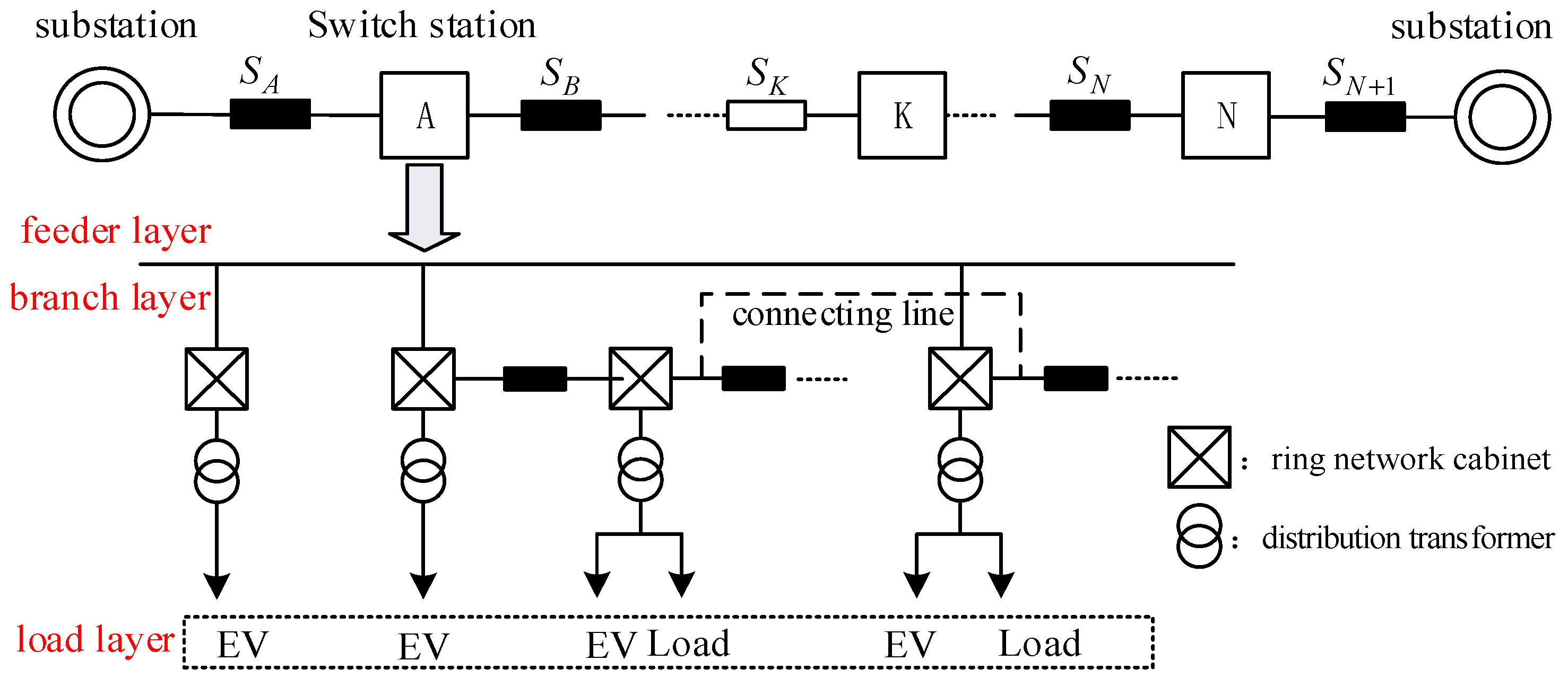
In Figure 1, A~N represent the switch station. The reconstruction between switch stations described in this paper means to change the state of disconnect switches and tie switches in the network to achieve regional load balance. The lower part of the arrow represents the location information of the specific load node under the switch station. The ring network cabinet adopts the interval power supply mode, and its branches can be directly connected to the distribution transformer, that is, directly supply power to the low voltage transformer area, and can also be connected to the ring network cabinet for external distribution.

The feeder voltage level in the structure diagram described in Figure 1 is 10 kV. Different numbers of EVs are installed under different distribution transformers. In view of the large number of electric vehicles in the future, this paper gives priority to optimizing the topological structure, and then sets up multiple aggregators under the switch station to guide the charging time of a specific electric vehicle.

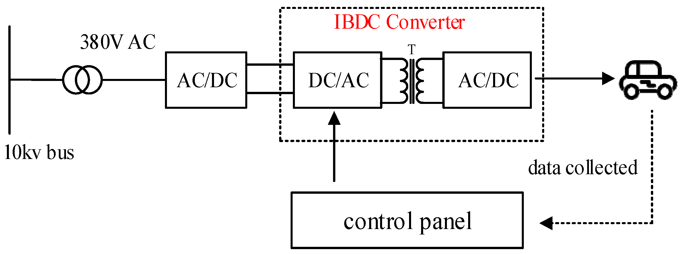
In this paper, the DC charging pile is used to charge the electric vehicle. The control panel in the charging pile is used to collect the battery capacity of the electric vehicle and upload the next day’s travel demand. The charging module uses IBDC converter to supply power to the high voltage distribution box in the vehicle. The structure of specific load layer is shown in Figure 2.

The driving circuit acts on the power switch to convert the DC voltage after rectifier filtering into AC voltage. Then, the AC voltage is isolated by the high frequency transformer, and the DC pulse is obtained by rectification filtering, thus charging the battery pack.

In this paper, the optimization between switching stations is defined as the feeder layer optimization, the optimization within the switching station is defined as the branch layer optimization, and the charging optimization for electric vehicles is defined as the load layer optimization.

2.1. Dynamic Reconstruction Model between Switch Station Groups

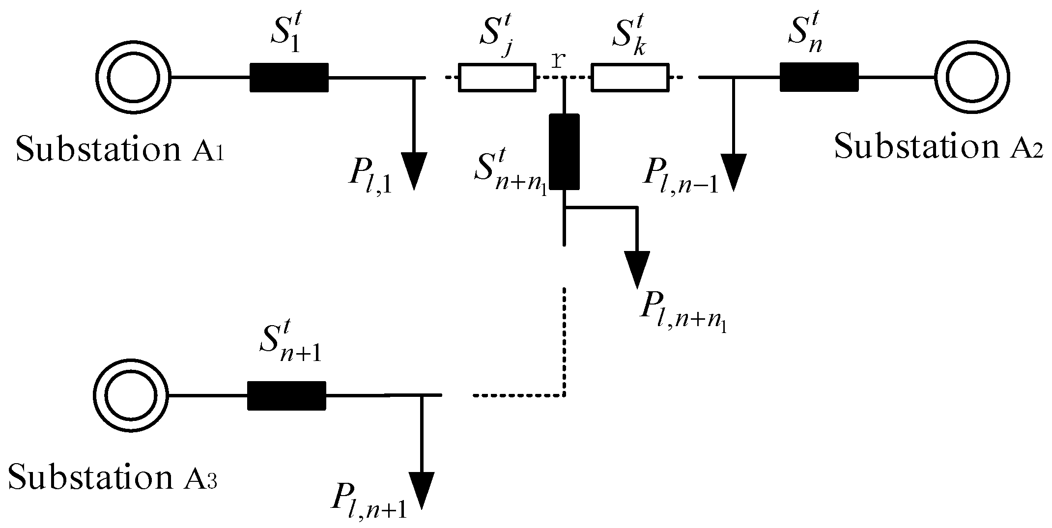
For the optimization of switch stations in feeder layer, it is necessary to analyze the connection mode of 10 kV distribution network, and derive different constraints for different connection modes. The actual typical connection types of 10 kV distribution network are single power supply, series supply, T-type series supply, etc. The feeder layer in Figure 1 is a series connection mode, this paper focuses on the analysis of T-type series supply wiring mode, which is more complicated. The specific connection mode is as follows.

Taking the switch topology of Figure 3 as an example, the power supply demand guarantee constraints are as follows:

$$\{\begin{array}{l}{P}_{\mathrm{G},{\mathrm{A}}_1}^t={\displaystyle \sum _{i=1}^{j-1}{S}_i^t{P}_{l,i}}\\ P_{\mathrm{G},{\mathrm{A}}_2}^t={\displaystyle \sum _{i=k+1}^n{S}_i^t{P}_{l,i-1}}\\ P_{\mathrm{G},{\mathrm{A}}_3}^t={\displaystyle \sum _{i=n+1}^{n+n_1}{S}_i^t{P}_{l,i}+{\displaystyle \sum _{i=j+1}^k{S}_i^t{P}_{l,i-1}}}\end{array}$$

(1)

where $P_{G,A_1}^t$ and $P_{G,A_2}^t$ represent all loads supplied by A₁ and A₂, respectively. P_l,i denotes the total load under the switching station after the i-th switch. $S_i^t$ represents the state of the i-th switch. t represents time.

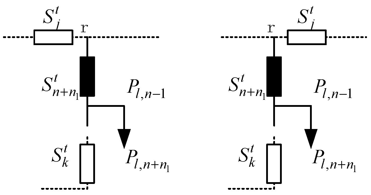
Three active power equality constraints ensure the power supply demand of each switch station. For the other two topologies, it is only equivalent to the change of power supply position. In the left graph of Figure 4, the original topology can be obtained by exchanging the position of A₂ point and A₃ point. In the right graph of Figure 4, the original topology can be obtained by exchanging the position of A₁ point and A₃ point.

For T-type serial supply structure, topology constraint is established:

$$\{\begin{array}{l}{\displaystyle \sum _{i=1}^{n+n_1}{S}_i^t=n+n_1-2}\\ n-2\le {\displaystyle \sum _{i=1}^n{S}_i^t\le n-1}\\ n_1-3+r\le {\displaystyle \sum _{i=1}^{r-1}{S}_i^t+{\displaystyle \sum _{i=n+1}^{n+n_1}{S}_i^t}\le n_1-2+r}\\ n_1+n-r-1\le {\displaystyle \sum _{i=r}^n{S}_i^t+{\displaystyle \sum _{i=n+1}^{n+n_1}{S}_i^t}\le n_1+n-r}\end{array}$$

(2)

Three inequality constraints ensure that there must be one or two disconnected switches between two power points, and equality constraints determine the number of disconnected switches in the T-type series supply structure. The three networks with different switch positions satisfy the constraint condition of Formula (2).

Therefore, according to the typical topology and connection mode of 10 kV main feeder, the total prediction load curve of each switch station is obtained. Taking the minimum load fluctuation level in the region as the goal, the reconstruction scheme between switching stations is established. The objective function is as follows:

$$f=\min {\displaystyle \sum _{t=1}^{24}\left[{\left(P_{G,A_1}^t-P_{G,A_2}^t\right)}^2+{\left(P_{G,A_1}^t-P_{G,A_3}^t\right)}^2+{\left(P_{G,A_3}^t-P_{G,A_2}^t\right)}^2\right]}$$

(3)

Considering the high cost of breaking the switch, this paper needs to calculate the load balancing index to determine whether to perform the switch action.

2.2. Internal Dynamic Reconfiguration Model of Switch Station

2.2.1. Branch Layer Reconstruction Model

After the feeder layer topology optimization is completed, it is necessary to analyze the load in each switch station to realize the branch layer autonomous optimization.

In this paper, the load curve of each ring network cabinet in the switching station is analyzed, and the minimum loss is achieved by changing the switch state between the ring network cabinets. At a single time level, the objective function of minimizing network loss is as follows:

$$f_{\mathrm{loss},i}={\displaystyle \sum _{\mathrm{Br}=1}^{N-1}{y}_{\mathrm{Br}}{r}_{\mathrm{Br}}}\frac{P_{\mathrm{Br}}^2+Q_{\mathrm{Br}}^2}{U_{\mathrm{Br}}^2}$$

(4)

where y_Br is the switch state of branch Br, 0 means open, 1 means close; U_Br is the voltage value at the beginning of branch; P_Br and Q_Br represent the injected active power and reactive power of the first node.

In addition, the power flow equation equality constraints, voltage amplitude constraints and line capacity constraints should be satisfied. The formula is as follows:

$$\{\begin{array}{l}{P}_{\mathrm{sum},i}=U_i{\displaystyle \sum _{j=2}^N{U}_j({\mathrm{G}}_{ij}\cos {\theta }_{ij}+{\mathrm{B}}_{ij}\sin {\theta }_{ij})}\\ Q_{\mathrm{sum},i}=U_i{\displaystyle \sum _{j=2}^N{U}_j({\mathrm{G}}_{ij}\cos {\theta }_{ij}+{\mathrm{B}}_{ij}\sin {\theta }_{ij})}\\ U_{i,\min }\le U_i\le U_{i,\max }\\ S_{\mathrm{Br}}^2\le S_{\mathrm{Br},\max }^2\end{array}$$

(5)

where S_Br,max is the maximum line capacity, U_i,max is the maximum node voltage.

In addition to the above constraints, the model also needs to meet the network topology operation constraints. In this paper, through network coding and simplification, a single-loop matrix is formed, which constitutes a radial constraint and a connected constraint, so as to determine the infeasible optimization solution.

The switches in each loop network are coded, and the single loop matrix is formed by searching the path from each node to the parent node. Each row in the single loop matrix represents a loop. The optimization variable in the reconstruction scheme is a switch in each row of the matrix. In order to make the solution satisfy the constraint of no-island and no-ring network, this paper uses SL correlation matrix and upper node search to determine the feasibility of each solution.

SL correlation matrix is defined as follows:

$$\mathrm{S}L=\left[\begin{array}{ccc}{a}_{11}& \cdots & a_{1n}\\ ⋮& \ddots & ⋮\\ a_{n1}& \cdots & a_{nn}\end{array}\right]$$

(6)

where a_ij represents the membership relationship between the j-th dimension solution and the i-th loop in the SL correlation matrix. If the solution belongs to this loop, it is 1, otherwise it is 0.

The principle of no-island judgment method is that if two rows are the same in the SL matrix, the solution of the j-dimension belongs to two loops at the same time. At this time, the system has a loop, and the infeasible solution must be eliminated.

The principle of upper node search is that the upper node of each node in turn is found, putting the result into a matrix, and finally it is judged whether there are 0 elements in the matrix except for the first column. If it exists, it means that there are islands in the network, and the infeasible solution must be eliminated.

Considering the high cost of the switch, this paper analyzes the difference between the network loss value before optimization and the optimized network loss value. Once the difference is less than a threshold, the switch optimization action is not performed.

2.2.2. Reconstruction Method Based on CNPSO Algorithm

Aiming at the branch layer dynamic reconstruction model, and in order to prevent particle swarm algorithm from falling into local optimum and accelerate the iterative speed, this paper improves the traditional particle swarm optimization algorithm by introducing logistic chaotic equation and niche elite retention algorithm. Refer to Appendix B for dynamic updates of inertia weights.

To solve the problem of local optimum, by adding a mixed disturbance near the group extremum, the solution space near the optimal solution is searched and the local search is strengthened. The specific steps are as follows:

Step 1: The global optimal solution of the n-th iteration output is mapped to the definition domain of the logistic equation to generate the chaotic variable z_nj. The formula is as follows:

$$z_j^n=\frac{x_j^n-x_{\min ,j}}{x_{\max ,j}-x_{\min ,j}},j=1,2,\dots \dots d$$

(7)

where x_j is the global optimal particle, that is, the disconnected switch combination of loops, n is the number of iterations; x_{max, j} and x_{min, j} represent the upper and lower bounds of the j-th dimensional variable, respectively.

Step 2: Using logistic mapping equation to generate d chaotic sequences, and then the chaotic variables are inversed to the original solution space to obtain new optimization variables. The formula is as follows:

$$z_j^{n+1}=\mu z_j^n(1-z_j^n),j=1,2,\dots \dots d$$

(8)

$$x_j^{n+1}=x_{\min ,j}+z_j^{n+1}\left(x_{\max ,j}-x_{\min ,j}\right),j=1,2,\dots \dots d$$

(9)

Step 3: The fitness function value of the new optimization variable is calculated and compared with the fitness value of the original solution x_j. If it is better than the original solution or reaches the maximum number of iterations, the position of the original particle is replaced by the position of the new particle. Otherwise, let n = n + 1, and turn to Step 2.

In addition to the local optimal problem, once the population is too large, it will affect the iteration speed. In this paper, the niche technology of sharing fitness mechanism is used to solve, that is, by calculating the sharing degree of individual particles in the group. The greater the degree of sharing, the higher the degree of closeness with other particles.

In this paper, the Euclidean distance between each particle is calculated, and the niche radius of the current population is calculated. The sharing degree of each individual is sorted, and the whole population is pruned. The individuals with higher sharing degree are deleted to ensure the uniform distribution of the solution. The number of all particles in the initial population is N_sh, and the shared fitness function is defined as follows:

$$F_i=\frac{1}{{\displaystyle \sum _{j=1}^{N_{\mathrm{sh}}}1-{\left(\frac{D_{ij}}{{\sigma }_{\mathrm{share}}}\right)}^{\alpha }}},\begin{array}{cc}& i,j\in {\mathsf{\Omega }}_{N_{\mathrm{sh}}}\end{array}$$

(10)

where ${\mathsf{\Omega }}_{N_{\mathrm{sh}}}$ represents the whole group space, ${\sigma }_{share}$ represents the niche radius, D_ij represents the Euclidean distance between individual x_i and x_j, and d represents dimension of decision variables.

$$D_{ij}=\Vert X_i-X_j\Vert =\sqrt{{\displaystyle \sum _{d=1}^m{\left(x_{id}-x_{jd}\right)}^2}}\begin{array}{cc}& i,j\in {\mathsf{\Omega }}_{N_{\mathrm{sh}}}\end{array}$$

(11)

$${\sigma }_{\mathrm{share}}=\frac{1}{N_{\mathrm{sh}}}{\displaystyle \sum _{i=1}^{N_{\mathrm{sh}}}\min \left(D_{ij}\right)}\begin{array}{cc}& i\ne j\end{array},i,j\in {\mathsf{\Omega }}_{N_{\mathrm{sh}}}$$

(12)

3. Isolated Bidirectional DC–DC Converter Optimal Efficiency Model

According to the topological structure of the medium voltage distribution network group, after determining the topological structure of the feeder layer and the branch layer, the orderly charging modeling of electric vehicles in each switch station is carried out. However, the charging efficiency of electric vehicles is affected by the transmission loss of the DC–DC converter, which further affects the accuracy of formulating the charging timing strategy for electric vehicles. It is assumed that the charging power is 12 kW and the battery capacity is 80 kWh. If the charging efficiency is increased by 5%, an additional 3 kW can be charged. In some scenarios, the next-day travel demand of EVs can be met in advance, and the charging load at that time at the branch layer can be reduced.

Therefore, aiming at the problem of peak current and return power when single-phase-shift (SPS) control IBDC converter, this paper adopts dual-phase-shift control (DPS) method to establish an optimal efficiency calculation model.

3.1. Principle of Dual-Phase-Shift Control

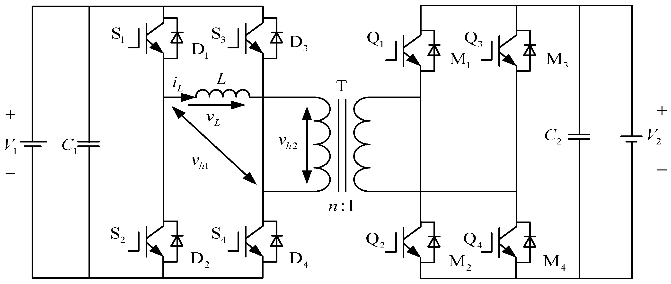
As shown in Figure 5, a typical IBDC converter circuit consists of two symmetrical H-bridges and high-frequency transformers. Compared with the traditional SPS control, DPS control is to introduce a new phase shift duty cycle between the two diagonal switch tubes of the full bridge on the primary side or on the secondary side. In this paper, the shift ratio D₁ of the primary side in a half period is defined as the internal shift ratio, and the shift ratio D₂ between the two sides in the half period is defined as the external shift ratio. When the internal shift ratio D₁ = 0, DPS control becomes traditional SPS control.

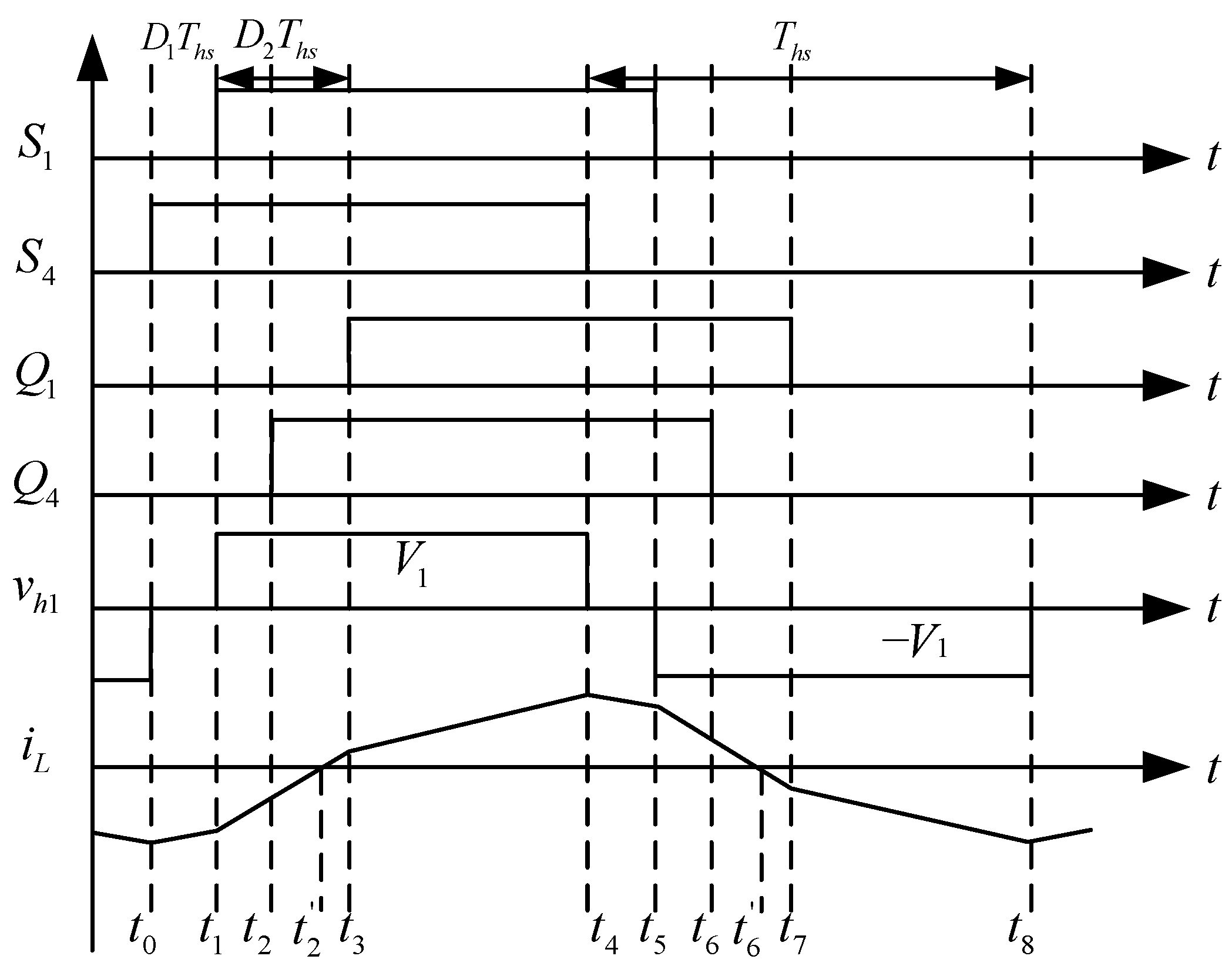
Figure 6 describes the working state of the converter in a switching cycle, such as the conduction time of the switch tube and diode, and the voltage change. Due to the symmetry of control, the system waveform of t₀–t₄ period is taken as the research object, and the working mode of converter can be divided into five states. According to the analysis of the working status of these five stages in turn, it can be found that the inductance current formula in the t₀–t₄ period is a piecewise linear formula.

When 0 ≤ D₁ ≤ D₂ ≤ 1, set t₀ = 0, and then other time point can be expressed as t₁ = D₁T_hs, t₂ = D₂T_hs, t₃ = (D₁ + D₂)T_hs, t₄ = T_hs, t₅ = (1 + D₁)T_hs, t₆ = (1 + D₂)T_hs, and t₇ = (1 + D₁ +D₂)T_hs. Voltage regulation ratio was set to k = V₁/(nV₂), and switching frequency was set to f_s = 1/(2T_hs). According to the symmetry, i_L(t₀) = −i_L(t₄) can be obtained, so the inductance current i_L(t) in each time period can be obtained, and then the following transmission power formula is derived by the inductance current formula:

$$P=\frac{1}{T_{hs}}{\displaystyle {\int }_0^{T_{hs}}{v}_{h_1}{i}_L\left(t\right)dt=\frac{n{V}_1{V}_2}{2f_{s}L}}\left[D_2\left(1-D_2\right)-\frac{1}{2}{D}_1^2\right]$$

(13)

3.2. Transmission Power Loss Model of IBDC Converter

The loss of an IBDC converter under DPS control mainly includes switching loss, conduction loss caused by switching devices, copper loss, and iron loss caused by magnetic components. The loss generated by the switching device is related to its on-state voltage drop and switching frequency. The loss generated by the magnetic element is related to the effective value of the inductance current and the winding resistance.

3.2.1. Switching Loss Model

When the switch tube works in soft switching mode, switching losses can be ignored. When the switch tube is in a hard switching state, due to the overlap of voltage waveform and current waveform in the transient process of opening and closing, the loss is generated [20]. The turn-off loss and turn-on loss are:

$$P_{off}=\frac{f_s{t}_{off}}{2}\left[\left(V_1+V_F\right){\displaystyle \sum _{t_s\in {\mathsf{\Omega }}_s}\left|i_L\left(t_s\right)\right|}+n\left(V_2+V_F\right){\displaystyle \sum _{t_Q\in {\mathsf{\Omega }}_Q}\left|i_L\left(t_Q\right)\right|}\right]$$

(14)

$$P_{on}=\frac{f_s{t}_{on}}{2}n\left(V_2+V_F\right)\left(\left|i_L\left(t_2\right)\right|+\left|i_L\left(t_6\right)\right|\right)$$

(15)

where t_off and t_on are switch turn-off time and turn-on time, respectively, and V_F is the forward voltage drop of diode. ${\mathsf{\Omega }}_s$ and ${\mathsf{\Omega }}_Q$ indicate the set of turn-off moments.

3.2.2. Conduction Loss Model

Since both the switch tube and the diode have a forward voltage drop when they are turned on, the on-state loss will be generated when the current flows, which is manifested in the form of heat.

Based on the odd symmetry of the converter working waveform and the conduction state of the switches and diodes in each stage, the conduction loss of IGBT and diode can be obtained [21]:

$$P_I=\frac{V_{sat}}{T_{hs}}\left({\displaystyle {\int }_{t_o}^t\left|i_L\left(t\right)\right|dt+2{\displaystyle {\int }_{t_{{}_2}^{\prime }}^t\left|i_L\left(t\right)\right|dt+}}{\displaystyle {\int }_{t_2}^{t3}n\left|i_L\left(t\right)\right|dt}\right)$$

(16)

$$P_d=\frac{V_F}{T_{hs}}[{\displaystyle {\int }_{t_o}^{t_1}\left|i_L\left(t\right)\right|dt+2{\displaystyle {\int }_{t_1}^{t_{{}_2}^{\prime }}\left|i_L\left(t\right)\right|}}dt+2{\displaystyle {\int }_{t_0}^{t_2}n\left|i_L\left(t\right)\right|}dt+{\displaystyle {\int }_{t2}^{t3}n\left|i_L\left(t\right)\right|}dt+2{\displaystyle {\int }_{t3}^{t4}n\left|i_L\left(t\right)\right|}dt]$$

(17)

where V_sat represents the on-state voltage drop of IGBT, which is a constant.

3.2.3. Magnetic Components Loss Model

Magnetic components mainly include transformers and auxiliary inductance, and the loss that produced during their work are mainly composed of copper loss and iron loss [22].

During the whole switching period, the current i_L flows through the transformer and the auxiliary inductance, and the copper loss is related to the root mean square of the current i_L:

$$P_{cop}=\left(R_{tr}+R_{au}\right)I_{rms}^2$$

(18)

where R_tr and R_au are winding resistance of the transformer and auxiliary inductor, respectively, which are constants. I_rms represents the root mean square of the current i_L.

Iron loss of magnetic components is mainly composed of hysteresis loss, eddy current loss, and residual loss. The calculation formula is as follows:

$$P_{iron}=\frac{2m{f}_s{\mu }_0^2{N}^2{V}_e}{g^2}{I}_{rms}^2$$

(19)

where m is the iron loss coefficient, ${\mu }_0^{}$ is the vacuum permeability, g is the air gap, N is the turns of the coil, and V_e is the effective volume. These parameters can be found from the parameter table [23].

3.3. Optimal Efficiency Calculation Model

According to Formulas (14)–(19), the switching loss P_SW, conduction loss P_CON, and transformer and auxiliary inductance loss P_TA of the IBDC converter can be obtained, so the total loss P_loss can be obtained. The detailed formula derivation is reflected in the Appendix A.

$$P_{loss}=P_{SW}+P_{CON}+P_{TA}$$

(20)

Therefore, the total loss P_loss under the control of DPS is related to the internal shift ratio D₁ and the external shift ratio D₂. This paper establishes an optimal efficiency model to select the optimal parameters D₁ and D₂ for a specific transmission power.

The efficiency of IBDC converter is defined as the percentage of the ratio of output power to input power:

$$\eta =\frac{P}{P+P_{loss}}$$

(21)

It can be seen from Formula (13) that the given transmission power P₀ can be obtained by various combinations of D₁ and D₂, but the total loss of the converter is different under each combination, so its efficiency is also different. In order to obtain the combination of D₁, D₂ corresponding to the minimum total loss of the converter, the Lagrange function can be established:

$$L\left(D_1,D_2,\lambda \right)=P_{loss}\left(D_1,D_2\right)+\lambda \left[P\left(D_1,D_2\right)-P_0\right]$$

(22)

Formula (22) is solved to find the optimal total loss value. The calculation formula is as follows:

$$\{\begin{array}{l}\frac{\partial L}{\partial D_1}=\frac{\partial P_{SW}}{\partial D_1}+\frac{\partial p_{CON}}{\partial D_1}+\frac{\partial p_{TA}}{\partial D_1}+\lambda \frac{\partial p}{\partial D_1}=0\\ \frac{\partial L}{\partial D_2}=\frac{\partial P_{SW}}{\partial D_2}+\frac{\partial P_{CON}}{\partial D_2}+\frac{\partial P_{TA}}{\partial D_2}+\lambda \frac{\partial P}{\partial D_2}=0\\ \frac{\partial L}{\partial \lambda }=P\left(D_1,D_2\right)-P_0=0\end{array}$$

(23)

By substituting Formulas (13) and (19) into Formula (23) and solving the root of the above equations, the optimal combination (D₁, D₂), and the efficiency of the IBDC converter reaches the maximum.

4. Orderly Charging Model of EV Considering IBDC Converter Optimal Efficiency

At the load layer, this paper takes the electric vehicles under the switch station as the research object. In this paper, a double-layer optimal scheduling model for EVs is established based on the distributed scheduling architecture.

4.1. Multi-Level Information Interaction Mechanism

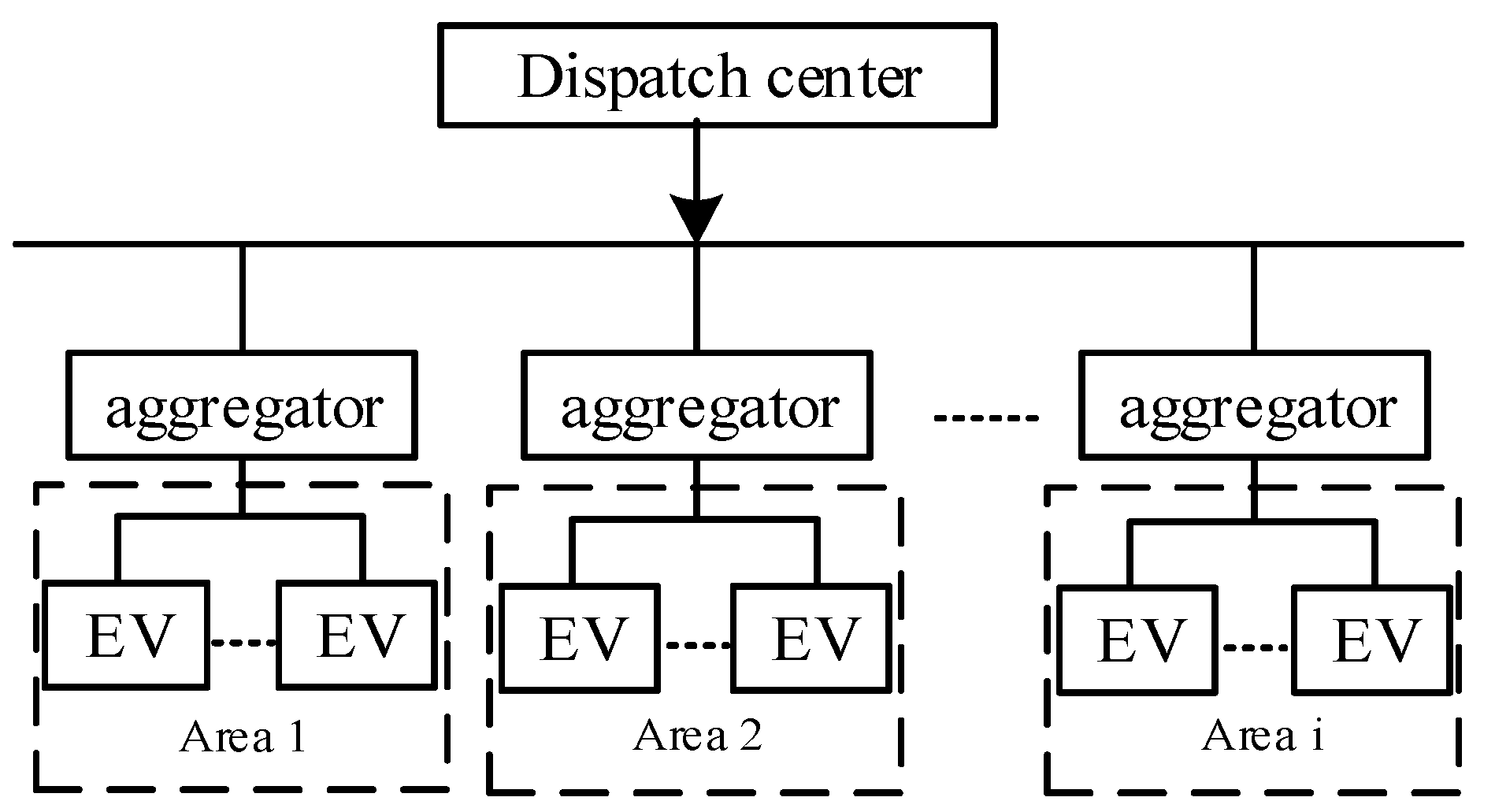
The principle of distributed scheduling is as follows: each switch station can further decompose all transformer area into several areas according to their geographic location, each area is dispatched by aggregators, and all aggregators accept the instructions of the dispatch center.

As shown in Figure 7, under the switch station, electric vehicle aggregators spanning multiple transformer areas are set up as an information bridge between a single electric vehicle and the dispatch center. It not only implements the instructions of the upper-level dispatch center, but also guides the lower-level specific electric vehicle charging time. The aggregators autonomy model facilitates centralized management of electric vehicles in the same area, avoiding the problems of low efficiency and huge data volume caused by the direct dispatch of each electric vehicle by the dispatch center.

The steps of the multi-level interaction mechanism are as follows:

Step 1: The user’s charging pile uploads the daily time when the electric vehicle is connected to the system, the state of charge at the time of connection, and the time when the user is expected to leave the system to the aggregator.

Step 2: Each aggregator obtains information about all electric vehicles in the area under its jurisdiction, and the dispatch center formulates demand targets according to the data integration of each aggregator so as to issue a dispatch plan for each time period to each aggregator.

Step 3: Based on the data uploaded by each electric vehicle, each aggregator’s scheduling goal not only requires the minimum variance of the load level under the switch station, but also requires the minimum sum of deviations between the actual scheduling results of each aggregator and the scheduling plan determined by the scheduling center.

Step 4: Under each aggregator, by controlling the charging time of all electric vehicles in the area, the deviation between the upper-level scheduling plan and the actual scheduling results of the lower-level electric vehicles is minimized, and step 4 is returned until the given convergence condition is reached.

4.2. Upper-Level Dispatch Model Considering Load Balance under the Switch Station

The upper-level dispatch model fully considers the overall load fluctuation level under the switch station, and realizes peak-shaving and valley-filling by formulating a reasonable dispatch plan. Therefore, for the topological structure of the branch layer, the upper-level objective function is established. The specific expression is as follows:

$$F_{\mathrm{up}}=\frac{1}{T}{\displaystyle \sum _{t=1}^T{\left(P_{\mathrm{L},t}+{\displaystyle \sum _{j=1}^N{x}_{j,t}}-\frac{1}{T}{\displaystyle \sum _{t=1}^T\left(P_{\mathrm{L},t}+{\displaystyle \sum _{j=1}^{N_0}{x}_{j,t}}\right)}\right)}^2}+\lambda {\displaystyle \sum _{j=1}^N\left({\displaystyle \sum _{t=1}^T{\left(P_{j,t}-x_{j,t}\right)}^2}\right)}$$

(24)

where P_L,t represents the original load level at time t in the network; x_j,t represents the scheduling plan of the j-th aggregator at the branch layer at time t; P_j,t represents the actual scheduling result of j-th aggregator; N represents the total number of aggregators in a certain switch station; and $\lambda$ represents the penalty coefficient, which is used to restrict the deviation between the actual scheduling result and the scheduling plan.

In addition to satisfying power flow equation constraints and voltage constraints, the other upper-level model constraints are as follows:

$$0\le x_{j,t}\le {\displaystyle \sum _{i=1}^n{P}_{j,i,\mathrm{ch}}{y}_{j,i,t}}\begin{array}{cc}& \forall t\in \left[1,\mathrm{T}\right]\end{array}$$

(25)

where P_j,i,ch represents the charging power of the i-th electric vehicle under the j-th aggregator; y_j,i,t represents the state of the i-th electric vehicle under the j-th aggregator connecting to the network at time t; the value is 1 when it is connected (may participate in the operation of the distribution network or not), and 0 when it is not connected.

4.3. Lower-Level Scheduling Model

In the lower-level dispatch model, this article considers the transmission power loss of the IBDC converter, and selects the optimal parameters D₁ and D₂ for a specific transmission power. In addition, the target of the lower model is taken as a part of the objective function of the upper-level. Each aggregator receives the dispatching instructions from the dispatch center, and the objective is to minimize the deviation between the actual dispatching results of all electric vehicles, which under the jurisdiction of each aggregator and the dispatching plan. For the j-th aggregator, the objective function is as follows:

$$F_{\mathrm{low}}={\displaystyle \sum _{t=1}^T{\left({\displaystyle \sum _{i=1}^n{P}_{j,i,\mathrm{ch}}{y}_{j,i,t}}-x_{j,t}\right)}^2}$$

(26)

where P_j,i,ch represents the rated charging power of the i-th electric vehicle under the j-th aggregator; y_j,i,t represents whether the i-th electric vehicle under the j-th aggregator participates in the dispatching of the distribution network at time t.

The constraints are as follows:

$$y_{j,i,t}=0\hspace{0.17em}\hspace{0.17em}\hspace{0.17em}t>t_{j,i,\mathrm{dep}}\parallel t<t_{j,i,\mathrm{arr}}$$

(27)

where t_j,i,dep and t_j,i,arr, respectively, represent the time when the i-th electric vehicle under the j-th aggregator is connected to the system on the same day (may participate in the distribution network operation or not), and the time when it is off the grid the next day is used to restrict off-grid electric vehicles from participating in distribution network dispatching.

$$S_{j,i,t_{\mathrm{dep}}}\ge 0.9S_{\mathrm{ev},\max }$$

(28)

$$0⩽S_{j,i,t}⩽S_{\mathrm{ev},\max }$$

(29)

where S_ev,max represents the maximum capacity of electric vehicles. Formula (28) is to meet the next day’s driving capacity demand, and Formula (29) is to prevent electric vehicles from overcharging.

$$S_{j,i,t+1}=S_{j,i,t}+{\eta }_{\mathrm{ch}}{P}_{j,i,\mathrm{ch}}\mathsf{\Delta }t$$

(30)

where S_j,i,t represents the SOC of the i-th electric vehicle at time t; $\mathsf{\Delta }t$ represents a period of time, the value is 1; ${\eta }_{\mathrm{ch}}$ represents the charging efficiency, and this parameter is determined by Formula (23) in Section 3. With a given transmission power, find the optimal D₁ and D₂ to minimize the power transmission loss of the IBDC converter and obtain the optimal efficiency ${\eta }_{\mathrm{ch}}$.

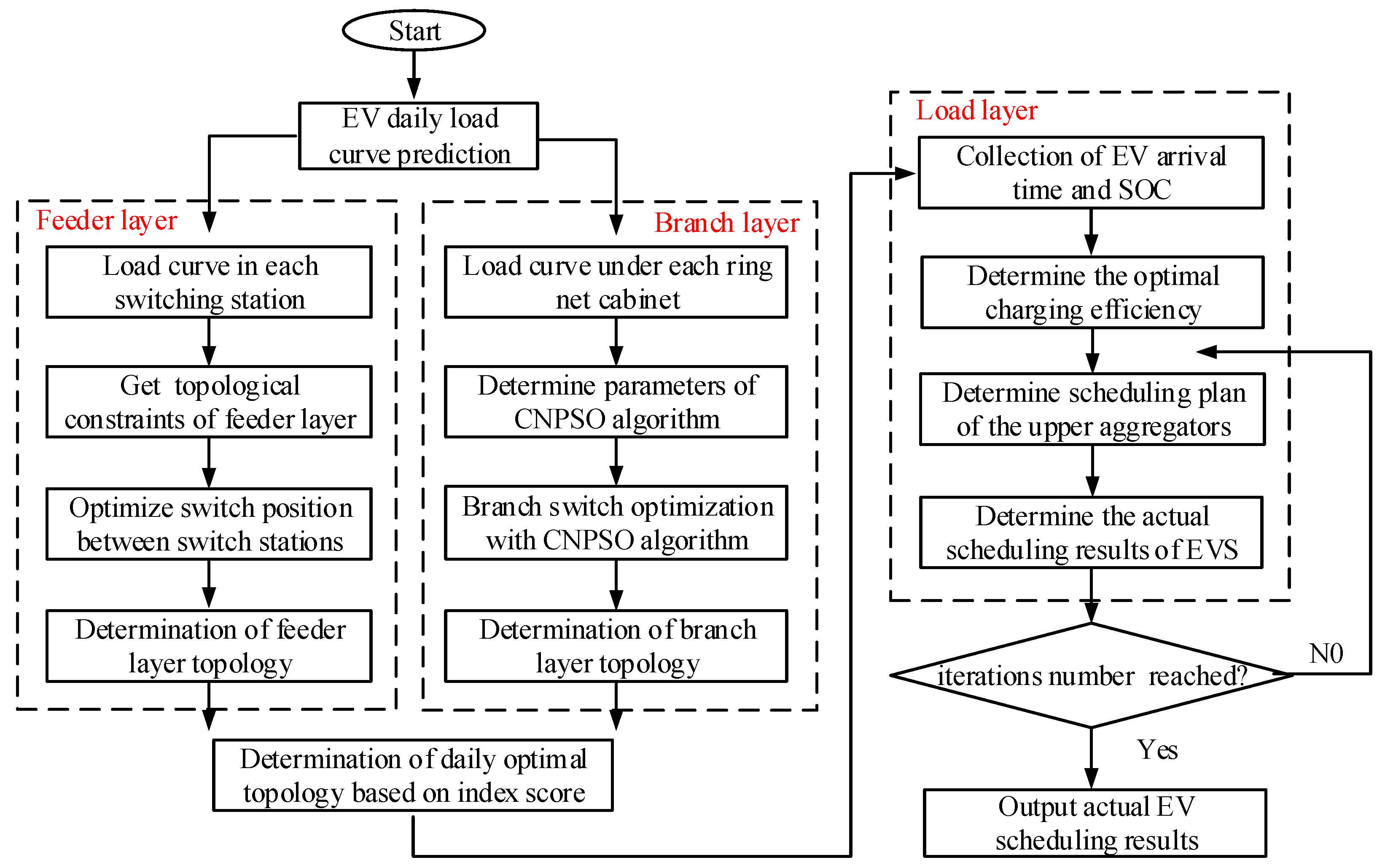
4.4. Overall Flow Chart of Hierarchical and Partitioned Optimization

This paper proposes an EV double-layer scheduling model based on the IBDC converter optimal efficiency model, and establishes the hierarchical and partitioned optimization model of the feeder–branch–load layer. The specific flow chart is shown in Figure 8:

5. Case Study

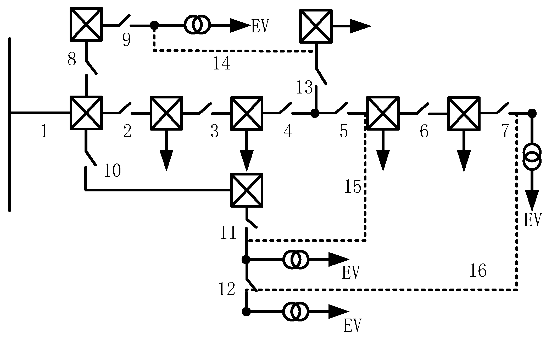
In order to verify the effectiveness of the proposed dynamic reconfiguration and electric vehicle scheduling model, this paper analyzes the cases in Figure 9 and Figure 10 on MATLAB R2014b. The system structure diagram is 10 kV medium voltage distribution network diagram. In Figure 9, the power point is 35 kV substation, and the shadow part is different switching stations. The network contains five switches on the main feeder. In the initial state, the black switch represents the closed state, and the white switch represents the breaking state. In Figure 10, the switch station contains 13 segmented switches and three tie switches, and three dispatching aggregators are configured. The dispatching aggregators manage 100 electric vehicles, respectively, and the tie switches 14, 15, and 16 are all disconnected before optimization.

The parameters of electric vehicle are as follows: the average charging power is 12 kW, the charging efficiency is 90%, the average battery capacity is 60 kWh, the upper limit of battery SOC is 95%, and the lower limit is 5%. For the calculation process and results of the orderly charging model of electric vehicles, this paper adopts the per unit (pu) value to facilitate calculation and explanation.

5.1. Optimization Results of Feeder Layer Reconstruction

The structure is powered by T-type series connection, and the Gurobi solver is called for optimization by analyzing the total load of each switch station in each period. In the actual simulation, the switch station near the substation is generally not used as the transfer object. The final switching operation number is 8, which can achieve load balancing of three substations. The results are shown in

Table 1. Comparison of feeder layer load balance.

Scenes	Time	Load Balance Degree	Switch State
Before optimization	10:00	26.285 MW	—
	20:00	28.466 MW	—
After optimization	10:00	24.922 MW	S2, S7 closed S3, S6 open
	20:00	16.235 MW	S3, S6 closed S2, S7 open

. Therefore, the load balancing level is improved by adjusting the switching state between switching stations, and the load difference of the three substations is minimized in one day.

5.2. Topology Reconstruction Results under Switch Station

Population sizepop = 100; iteration number N = 100; inertia weight is dynamic parameters. The threshold value is 0.1. It can be seen from

Table 2. Switch action before and after reconstruction.

Scenes	Time	Open Switch Number
Before reconfiguration	whole day	14, 15, 16
	5:00	14, 15, 12
After reconfiguration	12:00	5, 10, 15
	21:00	11, 15, 16

that after optimization, the switches 13, 14, and 15 are open during the period of 5:00 to 12:00, the switches 5, 10, and 15 are open during the period of 12:00 to 21:00, and the switches 11, 15, and 16 are open during the period of 21:00~24:00.

Assuming that the load connected to the lines numbered 4 and 5 in the original diagram are office buildings and other loads, the load is large during the day, so the network loss on lines 4 and 5 during the period after 12:00 is relatively large. At this time, it is necessary to open the line switch and the part of the load is transferred to the rest of the line for power supply.

Table 3. Switch action before and after reconstruction.

Scenes	Value of Network Loss	Improvement Rate
Before reconfiguration	202.5193 kWh	—
After reconfiguration	139.5191 kWh	31.11%

shows the changes in the network loss before and after optimization. The network loss is reduced by 17.42%, which shows that the network loss of the branch layer can also be reduced by adjusting the switch state.

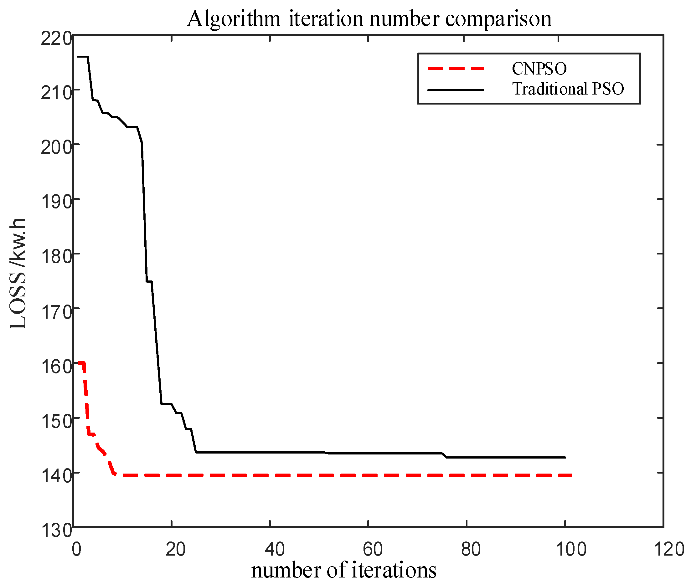
It can be seen from Figure 11 that the traditional particle swarm optimization algorithm may fall into local optimum and the iteration speed is slow. However, in the case of increasing the population size, the algorithm proposed in this paper makes iterative speed faster by deleting individuals with a higher degree of sharing. The average number of iterations can reach convergence at about 10 times. Moreover, while ensuring the speed, the global optimal solution is ensured by adding a mixed disturbance near the group extreme value. Therefore, the improved algorithm in this paper is more accurate and efficient.

5.3. Orderly Charging Results of Electric Vehicles

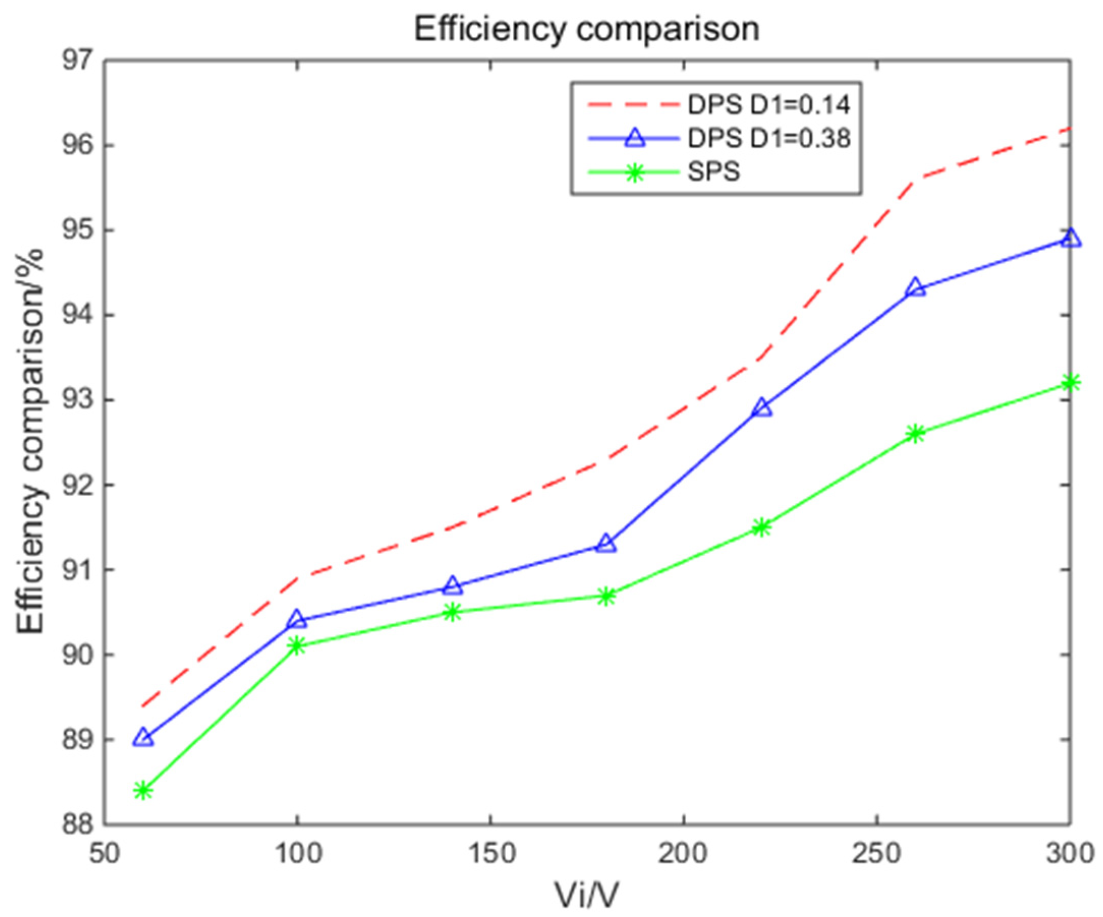
The simulation parameters of the converter in this article are as follows: load R = 100 Ω, DC capacitance C₁ = C₂ = 2200 $\mathsf{\mu }\mathrm{F}$, switching frequency f_s = 20 kHz, and transformer leakage inductance L = 7.7 $\mathsf{\mu }\mathrm{H}$. It can be seen from Figure 12 that when the power of 60 kW is given, D1 = 0.14, and the efficiency reaches the highest. The output voltage of electric vehicle is 300 V in this paper, so the optimal efficiency in the ordered charging model in this paper is 96.2%.

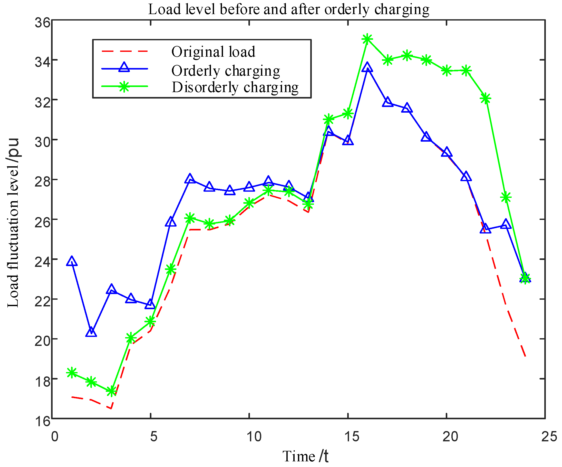
The switch station is mostly residential areas. It can be seen from the Figure 13 that electric vehicles were originally charged from 16:00 to 22:00, that is, the electric vehicles are charged immediately when residents arrive home. At this time, it is superimposed with other original loads, resulting in a large load under the switch station during this period of time. In addition, residents use less electricity at night, and electric vehicles are already fully charged, so the load is very small from 0:00 to 5:00, resulting in a large peak-to-valley difference in a day. After optimization, it can be seen from Figure 13 that the peak–valley difference is reduced from the original 16.5026 to 13.3174, which greatly improves the load stability of the branch layer and alleviates the phenomenon of adding peaks on the peak.

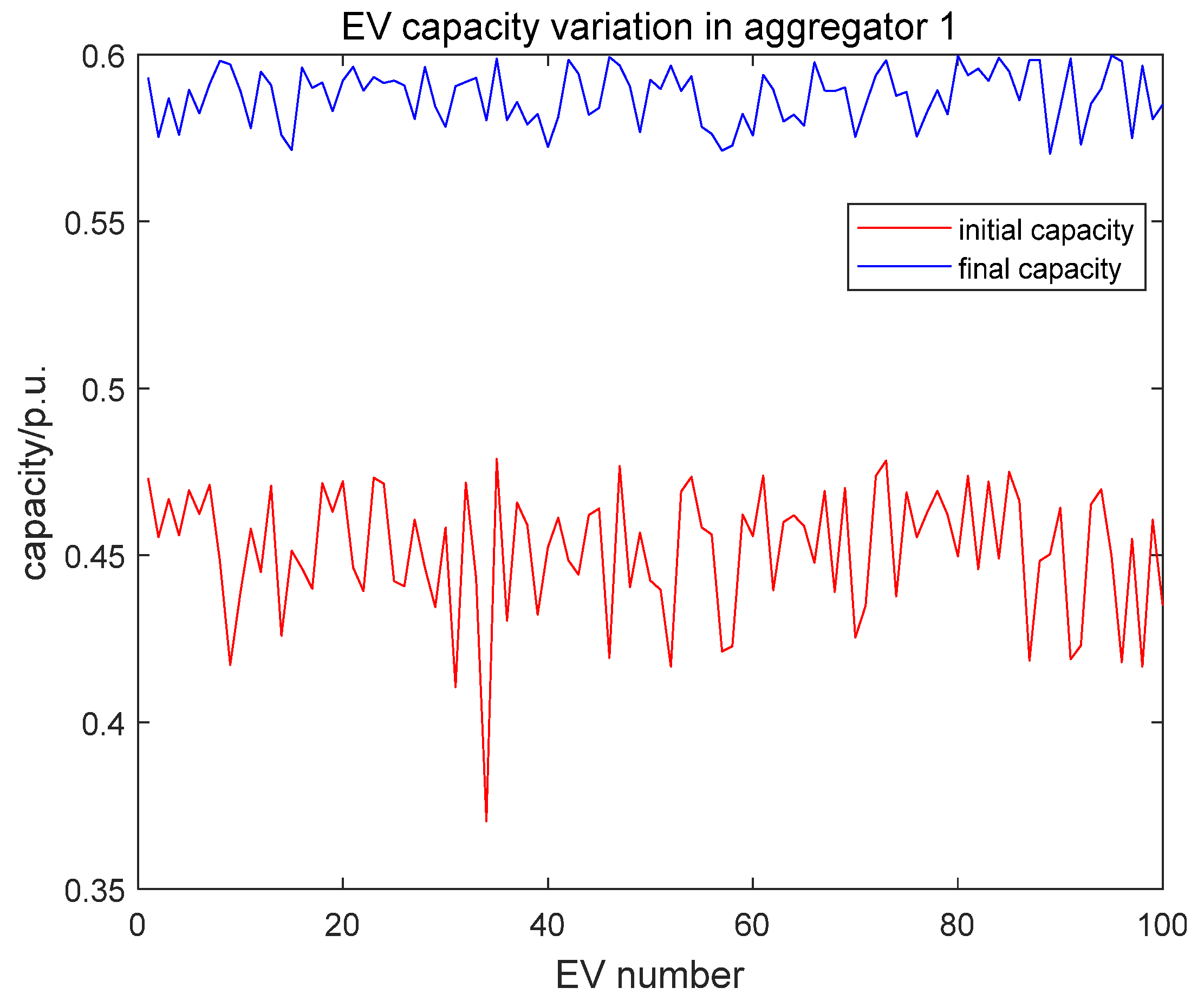
Figure 14 shows the initial capacity and the capacity after the final optimization of all electric vehicles in aggregator 1. In this paper, the travel scenarios of electric vehicles are divided into three types by analyzing the arrival time and expected travel time of electric vehicles. Figure 14 illustrates that no matter when the electric vehicle is connected, the optimization model in this article can guarantee the travel demand of the electric vehicle the next day.

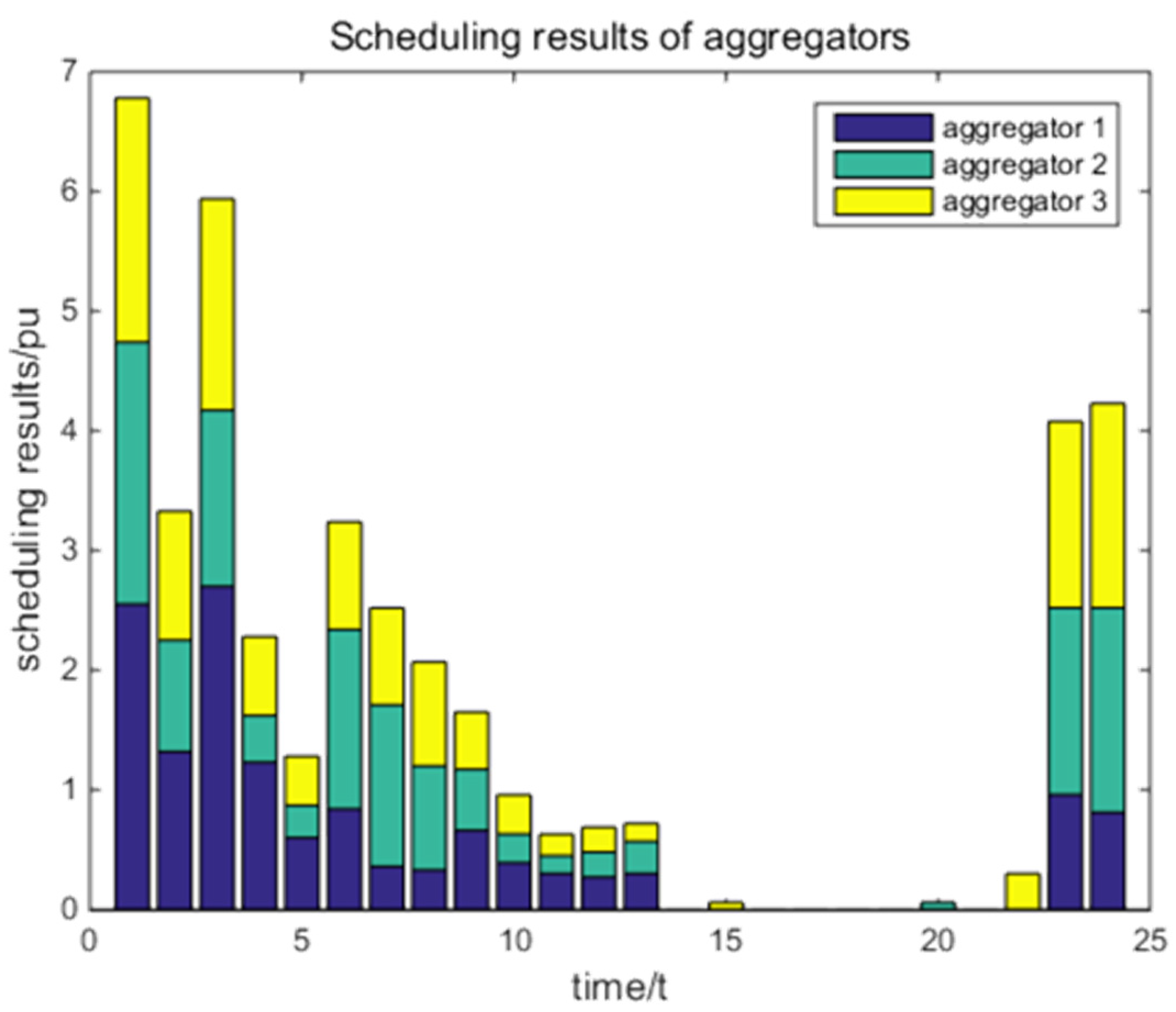
After the aggregator receives the dispatching instruction from the dispatch center, through double-layer optimization iteration, the actual dispatch results of the three aggregators is shown in Figure 15. The low cost of electricity at night and low load levels cause the charging behavior to be more frequent from 0:00 to 10:00 and after 22:00. By formulating a reasonable orderly charging strategy, the original disordered state of “plug and play” is changed. On the premise of meeting the demand of all EVs on the next day, the EVs connected during the peak power consumption period are arranged to be charged at night, which not only improves the load level at night, but also eases the power shortage during the peak power consumption period.

6. Conclusions

With the access of large-scale EVs in the future, it will inevitably increase the network loss of the medium-voltage distribution network and aggravate the imbalance of the distribution network load. In order to improve this situation, this paper proposes a three-layer optimization model from the perspectives of network structure and load itself. Each layer has its own findings with different priorities. The specific conclusions are as follows.

Firstly, at the feeder layer, this paper takes the connection relationship between switching stations as the research object, and establishes the dynamic reconstruction model between stations. By solving this model, it realizes the equalization of the load carried by the substation and avoids the occurrence of continuous heavy load in a certain substation. Secondly, at the branch layer, this paper takes the topology structure under a certain switch station as the research object, and a dynamic reconstruction plan is formulated for the topology structure. By solving this model, the branch layer network loss is effectively reduced, and the loss reduction rate reaches 31.11%. At the same time, this paper adopts the CNPSO algorithm to adapt to the larger branch topology scale in the future. This algorithm avoids the algorithm trapped in local optimum and improves the iterative speed by nearly 20%. Finally, at the load layer, this paper takes the electric vehicles under the switch station as the research object. The first step is to establish an IBDC converter optimal efficiency model, accurately calculating the charging power of electric vehicles in each period. The second step is to establish a double-layer distributed optimization scheduling model, which not only effectively reduces the difficulty of directly dispatching large-scale electric vehicles by dispatch center, but also formulates a reasonable charging strategy, achieving a 19.3% reduction in peak-to-valley difference. The findings of this paper are based on the consideration of all the major links in the medium-voltage distribution network, including branch layer network loss and optimal charging efficiency, which are rarely studied before. All of these should be present when solving the problems of medium-voltage distribution network loss and load fluctuation.