1. Introduction
The growing share of renewable energy generation based on fluctuating wind and solar energy sources poses an increasing challenge for the stability of the electrical power grid in Germany. This manifests in several indicators. For example, the amount of unused energy from renewable energy sources caused by necessary feed-in measures of the system operator has increased significantly, from 555 GWh in 2013 to 5404 GWh in 2018 [
1] (p. 158). This is the case even though the targets for the expansion of renewables have not yet been reached to achieve climate goals [
2,
3]. Furthermore, the number of hours with negative prices for electrical energy on the spot markets have risen over the last years [
4]. This shows that electricity consumers today are not able to react quickly enough to changes in electricity generation. To achieve a 100% renewable energy system, energy storage capacities and power grids must be expanded, and consumers must be enabled to adjust their demand in response to external signals or internal goals [
5]. The latter is referred to as demand-side management (DSM) and comprises all measures to influence energy demand, including measures to increase energy efficiency and energy flexibility [
6]. In principle, energy grids can be considered, such as the electric grid and the natural gas network. However, since the challenge in the case of electrical energy is to always balance supply and demand in the grid, this paper focuses on the electricity purchased by industrial consumers. Industry in Germany has a share of 45.7 % of the electricity demand and is thus the sector that promises the greatest leverage for increasing demand flexibility [
7].
In addition to classical electrical industrial processes, thermal applications supplied with electricity could provide further potential for energy flexibility in the future. Heating and cooling account for over 75% of final energy consumption in the industrial sector [
8]. Due to existing thermal storage capacities, thermal supply systems offer great potential for electrical DSM if the heating or cooling energy is generated with electrical energy converters [
9]. Electrification of thermal applications is also being pursued with a view to general decarbonization, since currently at least 72% of the process heat demand in industry is covered by fossil energy sources and is consequently associated with significant greenhouse gas emissions [
8]. To provide large amounts of heat at high temperature levels, steam is usually used as heat transfer medium, since it provides large amounts of latent energy at high condensing temperatures and heat transfer coefficients [
10] (p. 638). This applies especially to energy-intensive sectors such as the chemical industry, paper and metal production and food industries, which require high temperatures for their processes [
11] (p. 225). These industries use large proportions of their energy requirements in steam production. For example, the share in the US food industry is 57%, in pulp and paper production 81%, in the chemical industry 41% and in petroleum refining 23% [
12]. In addition to providing process heat, thermal energy is needed for hot water generation and space heating. Often, if central steam generation is available, low-temperature applications, such as space heating, are also supplied with steam [
13] (p. 106). This paper presents a method to quantify the energy-flexibility potential of industrial steam supply systems, without backpressure and extraction condensing steam turbines, that can be used for the electrical power grid using dynamic simulation. For this purpose, the relevant preliminary work in this subject area is summarized in the next section.
2. Conceptualization
To evaluate the electrical DSM potential of industrial steam supply systems using a simulation-based approach, a concept for the analysis of this specific energy-flexibility potential was developed. Therefore, in this chapter, the basic topology and derived flexibility measures are explained as a framework for the later-presented simulation models. Furthermore, basic mechanisms of electricity markets, which enable the marketing of energy-flexibility measures, are outlined.
In the context of this work, industrial steam supply systems are divided into three subsystems: steam generation, steam distribution, and steam consumption [
26] (p. 11). Steam generation can be based on different primary energy sources, such as gas or electricity via boilers. If not generated within the industrial site, steam can also be procured from energy suppliers, e.g., from waste incineration plants. Steam distribution within one industrial site can be conducted by several distribution networks of varying pressure levels so that different temperature requirements in each network are satisfied. The steam for the distribution network is usually supplied at the highest required pressure level and then reduced via valves for steam networks with lower pressure levels [
25] (p. 193). Modern steam supply systems with a constant mass flow rate and pressure drops greater than 8 bar may use backpressure turbines to reduce the steam pressure in an energy efficient way [
27]. Due to the system age, steam turbines are not used at the investigated production site (see
Section 4). The distributed steam is used to meet the heating demand for several production processes as well as industrial buildings. Typically, in larger industrial sites, these consumers can be regarded as independent entities.
2.1. Energy-Flexibility Measures in Industrial Steam Supply Systems
To derive energy-flexibility measures of a steam supply system for flexibilizing the primary energy demand, all three subsystems and their interactions can be considered. Here, direct and indirect measures can be differentiated. Direct measures describe changing the topology or operating strategy of steam generation and distribution. Indirect measures require changes in the production processes or buildings to adapt to steam consumption. Assuming low transparency and difficulty in intervening in production processes, this work does not consider indirect measures that flexibilize the production processes and thus steam consumers [
25] (p. 193).
Regarding steam generation and distribution, three energy-flexibility measures for flexibilizing primary energy demand can be investigated [
28] (p. 5): bivalent steam generation, inherent energy storage and adjusting process parameters (see
Figure 1). For the first measure, a bivalent steam generation with two different steam generators, e.g., gas- and electricity-based boilers, must be implemented. In this case, the steam generation can be switched between gas or electricity as the primary energy source. The second energy-flexibility measure aims at storing energy by using the inherent storage capacity of the distribution network as well as steam generation. In addition, it is assumed that only a single electrical boiler is available. In this case, inherent storage can be performed by changing network parameters such as pressure level or temperature for a short period of time, resulting in changing electrical power consumption and thus an energy-flexibility potential. This is a transient measure, so subsequent higher or lower, energy consumption must take place after the request. The third energy-flexibility measure—adjusting process parameters—is a stationary measure because the energy-flexibility potential results from power differences in steady-state steam generation at different pressure or temperature levels. In this case, no higher or lower, energy consumption after the flexibility request is necessary. For this measure it is also assumed that the steam is generated by a single electrical boiler. For the application of all measures, it must be ensured that network restrictions regarding permissible pressure and temperature are always complied with. Dependent on distribution network restrictions as well as standard parameters and operating strategy of the steam supply system, a positive and negative energy-flexibility potential must be differentiated. The energy-flexibility potential is calculated as the difference between the electrical load profile of the primary energy sources at the flexible and the reference state. A positive potential is defined by the ability to reduce power and a negative one by the ability to increase power relative to the reference state [
28] (p. 5).
2.2. Marketing Energy-Flexibility Potentials
The economic potential of electrical DSM by applying the described energy-flexibility measures is highly dependent on market mechanisms [
29,
30]. Three mechanisms can be differentiated in relation to the flexibility of the steam supply system: costs of energy consumption, costs related to the load curve (power) and financial rewards for system services [
31] (pp. 273–277). The costs of energy consumption can be profitable for energy-flexibility measures if the market offers dynamic pricing, which means that prices for electric energy varies over time for the consumer (industrial site) [
32,
33,
34]. In the German electricity market, mainly large companies can profit from dynamic pricing models. Furthermore, taxation lowers the effect of varying prices, and typical electricity markets charge peak loads due to the importance of grid stability. If energy-flexibility measures can reduce such peak loads of the industrial site, this may offer a significant lever for reducing electricity costs [
35] (p. 7). Besides the consumption of electric energy, electricity markets can offer financial rewards for system services. If there is the risk that electric power generation and consumption in the network are not in balance, system services are mandatory to maintain system stability. Therefore, dedicated flexibility from consumers or plants are rewarded. To take part in the system service market, a complex admission procedure is necessary. The specific German market design considered in this work’s use case is further explained in
Section 4.
3. Dynamic Modeling of Industrial Steam Supply Systems
In this section, this work presents a modular simulation model to analyze the electrical DSM potential of industrial steam supply systems. First, the modeling of subsystems (steam generation, distribution and consumption) is described. Second, the modeling of the control mechanisms depending on the energy-flexibility measures is clarified.
3.1. Modeling Environment
To simulate the steam supply system, the object-oriented modeling language Modelica is used. All utilized component models are part of the Modelica Standard Library [
36]. For system modeling with Modelica, the system is decomposed into different components. Since the modeling of the overall system requires the interaction of the component models, it is necessary to define uniform ports and variables that are exchanged through these ports. The physical behavior of a component and the effect on these variables is described using differential-algebraic equations.
Because steam supply systems are fluid systems, they are modelled with the Modelica Fluid package. This package is based on the Modelica Fluidports for one-dimensional flow modeling. This means that the flow variables are discretized exclusively along one direction. Since the flow is a single substance flow, the variables absolute pressure, mass flow rate and specific enthalpy are necessary to describe the problem. The absolute pressure is a state variable, requiring the pressure in connected ports to be equal. On the other hand, the mass flow rate is a flow variable, meaning the connection of two or more ports restricts the sum of all flow rates to zero [
36]. The specific enthalpy is transported with the mass flow to consider the energy balance. In this section, only the basic modeling of components is described. The structure of the aggregate model containing the connected component models is not discussed, since this depends on the specific use case.
3.2. Modeling the Steam Generation
The system boundary representing feedwater entering the steam generation system is modeled by an ideal mass flow source of constant temperature, which keeps the feed water level in the steam generator constant. To model the evaporator, the equilibrium drum boiler model from the Modelica Standard Library is used [
36]. With Equation (1), the supplied heat flow
is calculated as a function of the operating point
, the nominal power
and the efficiency
, depending on the operating point. The efficiency
η(OP) also allows the consideration of internal steam consumption, e.g., for degassing. The boiler is controlled by a proportional controller.
To consider the dynamics of the generator, the operating point is passed through a PT
1-element [
36]. This delivers the step response
for a step function
at time
, with an amplification factor equal to one and the time constant
.
The modeling of a PT
1-element corresponds to the integration of a first order low pass filter. According to Equation (4), it is shown that, for
, 99.33% of the step
is reached, so it is assumed that the final system state is reached. With the rise time
, the time constant
is calculated as per Equation (5).
The introduced modeling strategy for calculating the supplied heat flow and considering the dynamics is also applied to model a superheater for reaching temperatures above the saturation temperature. Therefore, instead of the equilibrium drum boiler model, a fluid volume is used.
The steam conditioning valves are modeled with the isenthalpic linear valves of the Modelica Standard Library, controlled by proportional controllers. The dynamic behavior is considered using PT
1-elements. The pressure drop
is calculated using the mass flow rate
, the operating point
and the nominal parameters
, according to Equation (6).
3.3. Modeling the Steam Distribution
Modeling the steam distribution networks based on physical parameters like pipe lengths, diameters or bends requires significant effort in determining these parameters. Instead, a data driven method is used to approximate pressure and heat losses in the distribution network. The pressure losses throughout the pipe network are calculated by a regression model, using the approach in Equation (7), which is derived from a generic pressure loss model [
37] (p. 291). Therefore, a new pressure loss factor
is introduced, based on the pressure loss factor
, the fluid density
and the pipe cross-sectional area
.
To consider heat losses along a pipe section to the environment, the following linear approach is applied [
38] (p. 104). Accordingly, the heat flow rate
depends on the thermal resistance
, the mean fluid temperature
and the ambient temperature
. Using the new coefficient
to account for heat loss, the inlet temperature
is used for the regression model instead of the mean fluid temperature
.
3.4. Modeling the Steam Consumption
The modeling approach is chosen to be as generic as possible so it can be applied to steam supply systems with many different types of consumers, e.g., building heating systems as well as different types of production processes. Moreover, the simulation of different energy-flexibility measures and extensive parameter studies on annual data lead to high simulation performance requirements. Accordingly, the number of nontrivial linear and nonlinear equations should be reduced to a minimum, which is why throttles and their controllers are not modeled. Therefore, the generic steam consumer is modeled as an ideal mass flow sink, which receives a mass flow
from the steam distribution system. To calculate the heat energy consumed
, both the sensible energy and the pressure-dependent evaporation enthalpy
are considered [
38] (pp. 82–84, 199). To calculate the sensible energy, the mass flow
is multiplied by the specific heat capacity
as well as the temperature difference of the inflowing steam
and the saturation temperature
.
With this generic consumer model, energy efficiency can be investigated only superficially because process-specific effects such as subcooling are not considered. Since the consumer model remains constant for all energy-flexibility measures, changes in the energy efficiency of the system because of different generation technologies and states in the steam distribution can still be assessed. To calculate the energy efficiency of the entire system
, the heat power used by all consumers
is divided by the total power demand
.
3.5. Modeling the Control Mechanisms
Different operating strategies for all three flexibility measures must be implemented and tested to determine the energy-flexibility potential. In the case of bivalence and storing energy inherently, additional controllers are required. The mechanisms of these controllers are described in the following section (see
Figure 2).
The operating strategy for bivalent operation will only be explained for the evaporator; however, the strategy is analogous for the superheater. Bivalence in this case is established by the availability of an electric- and a gas-powered steam generator. The activation of an energy-flexibility potential is simulated by a rectangular function. A function value of +1 results from activating negative potential, resulting in a load increase, and a function value of −1 from activating positive potential, resulting in the load decreasing. Accordingly, the rectangular function only defines the direction of the energy-flexibility potential. To calculate the changes in electrical power consumption, this value is multiplied by the marketed energy-flexibility potential. The potential is added to the reference power at the time of activation to calculate the power demand of the electrical steam generator while the energy-flexibility measure is implemented. By dividing this value by the nominal power of the electrical steam generator, the operating point is calculated and passed on to the model of the electrical steam generator. During the flexible state, the electrical steam generator is controlled separately, according to the required flexibility, and the pressure control only affects the gas-powered steam generator. During the reference state, both steam generators are controlled by the pressure controller. To divide the total power between both generators, factors to determine the load-splitting shares during the reference state from 0 to 1 can be used.
For storing energy using inherent storage, the energy-flexibility potential results from the steam supply system’s capacity and not stationary changes in power consumption due to changed process parameters. Consequently, another model is required to quantify the energy-flexibility potential. In this case, pressure and temperature are increased or reduced. This results in an increase or reduction of the supplied power until the target state is reached. By integrating the power from the initial time of change until the target state is reached, the additional energy to reach the target state can be calculated, and thus the inherent storage capacity used. Through dividing the inherent storage capacity by the duration of an energy-flexibility measure, the possible change in electrical power consumption is calculated depending on the holding period, without violating network restrictions.
To quantify the energy-flexibility potential by adjusting the process parameters, no additional controller is needed. In this case, the target variables of the controllers are adjusted towards the upper or lower network restrictions in order to achieve stationary differences in electrical power demand for different process parameters.
4. Implementation of an Exemplary Use Case
This section explains the topology of the investigated steam supply system of a representative chemical company. The model parameterization and the technical validation are subsequently discussed. In
Section 4.4 the different marketing options for energy-flexibility potentials and further economic assumptions for the calculation of the economic energy-flexibility potential are presented.
4.1. Industrial Steam Supply System Topology
The investigated industrial steam supply system is characterized by a system topology consisting of central steam generation, distribution and consumption. First, superheated steam is generated by an evaporator and superheater. The steam is generated at the highest pressure level required by a consumer, which is about 13 bar for the investigated production site. In fact, pressures between 11.5 and 13.5 bar and temperatures between 200 and 230 degrees are tolerated for steam generation. According to
Section 2, these are the restrictions of the steam supply system that must be considered when implementing energy-flexibility measures. The steam is then distributed to the consumers via three different steam networks with pressure levels of 13, 7 and 3 bar, which is why the pressure for two of the steam networks is reduced by steam conditioning valves. The heat supply of buildings is carried out mainly via the 3 bar system, while the supply of production processes often requires higher condensation temperatures, which is why their supply is carried out via the 7 and 13 bar systems. The consumers receive the needed amount of steam through their respective valves, which causes the used steam to condense. The resulting condensate is collected in open condensate containers and then pumped back to the steam generator.
Figure 3 provides a simplified illustration of the steam supply system structure.
The consumers can be divided mainly into production processes and building heating systems. The production processes cause a nearly constant base load of the steam demand because they are continuously in operation, while the building heating leads to seasonal fluctuations. This can be shown by analyzing the total steam demand, as it correlates significantly with the weather conditions.
Figure 4 shows the daily average steam mass flow rate in tons per hour for the year 2019.
4.2. Parameterization
The parameters of the gas-powered components and the steam conditioning valves are taken from the data sheets of the installed components at the investigated production site. For the electrical components, the parameters of an industrial electrode boiler are used [
39]. Typical energy efficiency values of the different technologies are taken from [
40,
41]. The internal steam demand for degassing amounts to approx. 5%, which is why the parameters were adjusted according to
Section 3.2.
Table 1 gives an overview of the parameterization of the steam generation and
Table 2 summarizes the parameters of the steam conditioning valves.
The regression coefficients of the pipes in the steam distribution network are calculated with weekly average data from the year 2019 to reduce the influence of single outliers. Because of the large number of pipe sections, their respective coefficients are not listed at this point.
4.3. Validation
For all investigations, real consumption data for the year 2019 from the company’s energy monitoring system is used for the consumers’ mass flow rates within the model. The data is sampled into a quarter-hourly dataset. To validate the regression coefficients used to model the pipes in the distribution network, the root-mean-squared relative error of all pipe sections is determined. For the pressure loss model, the error amounts to 1.9%, for the heat loss model, it is 4.6%. Thus, the model of the distribution system fits well to the real conditions. The parameters of the gas-powered steam generator could not be validated in the real system since no operating data was available; instead, data sheets of the steam boiler were used for the validation.
4.4. Marketing Energy-Flexibility Potentials in Germany
Energy flexibility and its measures can only be feasible if they are economically profitable, which is highly dependent on the energy market. This work focuses on the German electricity market, for which the main market mechanisms are described in the following sections. The analysis of the market design and its possibilities is based mainly on the information in [
42] (pp. 10–17). After a general market description in
Section 4.4.1 and
Section 4.4.2,
Section 4.4.3 introduces the examined marketing options and further economic assumptions made for the simulation studies.
4.4.1. Reducing Costs of Energy Consumption—Spot Market
The German electricity market (without system services) is designed as an energy-only market, which means that only the physical delivery, and not the readiness to deliver electrical energy, is paid for. The market itself is divided into the spot and the over-the-counter (OTC) market. While short-term contracts are traded on the spot market, the OTC market also allows long-term price hedging. Since energy flexibility means the ability to quickly adapt a production system to the changes in an energy market, marketing energy flexibility is mainly aimed at the short-term spot market, which will be explained below [
28] (p. 4).
The spot market can be divided into the day-ahead market for trading delivery contracts for the next day and the intraday market for trading delivery contracts for the same day. The stakeholders of the spot market—mainly the European power exchange (EPEX SPOT SE)—are producers, suppliers, energy-intensive consumers, aggregators, network operators and trading companies [
43]. Bids for various products are placed daily in the day-ahead auction. After all demand and supply quantities have been sorted in descending and ascending order, the market clearance price is published. This price is determined by the point of intersection of supply and demand. It applies to all participants whose price is less than or equal to this price. The intraday market is divided into the opening auction and continuous trading. During the opening auction, quarter-hourly contracts are traded for the following day. Afterwards, the trading of other products starts. The price formation during the opening auction is carried out in the same way as on the day-ahead market, according to the unit pricing procedure. During continuous trading, the pay-as-bid procedure is applied, whereby the offered price must be paid.
4.4.2. Financial Rewards for System Services—Balancing Power Markets
For the stabilization of frequency, voltage and power loads in the power grid, system services are used. A system service for the stabilization of the grid frequency is the provision of balancing power, which is of particular interest in the context of energy flexibility studies. This service allows the synchronization of energy demand and supply after closing the spot market. If demand is greater than supply, positive balancing power is required and vice versa. There are different types of balancing power, which are mainly characterized by their prequalification process and price formation procedure; these are explained below. Primary balancing power must be fully available within 30 s and maintained for at least 15 min. Like the day-ahead auction, one market clearance price for reserving the balancing power applies to all participants who bid a lower price. The offer includes positive as well as negative balancing power, so the energy-flexibility potential must be available in both directions. Therefore, actually requesting the balancing power is not paid for, since positive and negative balancing energy is compensated over time. If 30 s after the occurrence of a disturbance no stabilization can be achieved by the primary balancing power, secondary balancing power is requested. This must be fully available within 5 min for up to 4 h. Secondary balancing power bids contain both a power price for the provision of balancing power and an energy price for the actual request of balancing energy. The bids are surcharged based on the power price, where a pay-as-bid procedure is used. Contrary to the primary balancing power, positive and negative balancing power can be offered separately. If stabilization cannot be achieved within 5 min by using primary and secondary balancing power, the minutes’ balancing power is activated. This must be fully available within 15 min for up to 4 h. The market for minutes’ balancing power is designed like the secondary balancing power market.
4.4.3. Examined Marketing Options and Further Economic Assumptions
For the simulation studies, marketing energy-flexibility potentials on the day-ahead market as well as on balancing power markets is investigated. Marketing on the day-ahead market is examined for all energy-flexibility measures. In this context, no special requirements are set for the activation period, and it is assumed that there is sufficient time to set the target state. For marketing energy-flexibility potentials as balancing power, it is assumed that only the power price for reserving the energy-flexibility potential is paid, since the actual demand for balancing energy and the resulting energy prices can only be forecast inaccurately. However, it can be assumed that the additional costs for requesting the energy-flexibility potential, e.g., through operating at a higher pressure level, are covered by the energy prices [
44] (p. 275). Furthermore, the price transformation procedure has a significant impact on the profitability of an energy-flexibility measure. This especially applies to pay-as-bid markets, as the revenues depend on the bidding strategy. For such markets, both the revenues achievable in the optimum case and the revenues achievable through a realistic bidding strategy are examined. This strategy means the price, which is bid in an auction, results from the marginal price of a previous auction, multiplied by a safety factor of 0.9. To calculate the revenues, the energy-flexibility potential quantified in the simulation is multiplied by the financial rewards or the differential costs in energy consumption. In the optimal case, it is assumed that the marginal price, consequently the highest financial reward or most favorable electricity price, is achieved in each auction. In a realistic case, it is considered that the bidding of an energy-flexibility potential may not be successful or may be successful, but the bid is lower than the marginal price.
Due to the complexity of the tax and levy system, the results of individual companies can vary greatly because of different exemption options. For this reason, the marginal cases of no exemption and the maximum possible exemption are calculated for an industrial customer with an annual consumption of the investigated use case. If no exemption can be achieved, taxes and levies excluding value added tax (VAT) can reach 116.5 €/MWh. If all possible reductions are realized, this amount is reduced to 9 €/MWh [
1] (p. 286).
5. Results
In the following section, both the technical and the economic results for the examined energy-flexibility measures are presented.
Section 5.1 covers energy-flexibility potential through operating with bivalent energy,
Section 5.2 through storing energy inherently and 5.3 through adjusting process parameters. Finally, the effects on energy efficiency of using different generation technologies and operating under different pressure and temperature conditions are examined.
5.1. Energy-Flexibility Potential via Bivalence
In the case of bivalent steam supply, the technical energy-flexibility potential depends on the rise time and the dynamic behavior of the steam generators. This is explained in the following text for the demand of negative secondary balancing power, but it can also be observed with other types of balancing power. When the energy-flexibility potential is requested, the electrical generator is started within the required rise time. Since the deactivation time of the gas-powered generator is much longer than that of the electrical steam generator, it cannot be shut down fast enough, even though the required power is already provided by the electrical generator. This leads to increasing steam pressure and violation of the pressure restriction. Thus, this is a theoretical energy-flexibility potential that is not fully available. Consequently, the amount of the energy-flexibility potential requested at the time of the restriction violation must be reduced until the pressure is within the permitted limits. In the simulation, this is realized by automated parameter studies reducing the energy-flexibility potential if the restrictions are violated. As soon as the requirements are met at all points in time, the technically permissible energy-flexibility potential is identified.
Figure 5 shows the theoretical and technical energy-flexibility potential (
) as well as the steam pressure for negative secondary balancing power.
The presented method is used for all types of balancing power. The energy-flexibility potential of the evaporator is optimized to maintain the pressure restriction, while that of the superheater is optimized to maintain the temperature restriction.
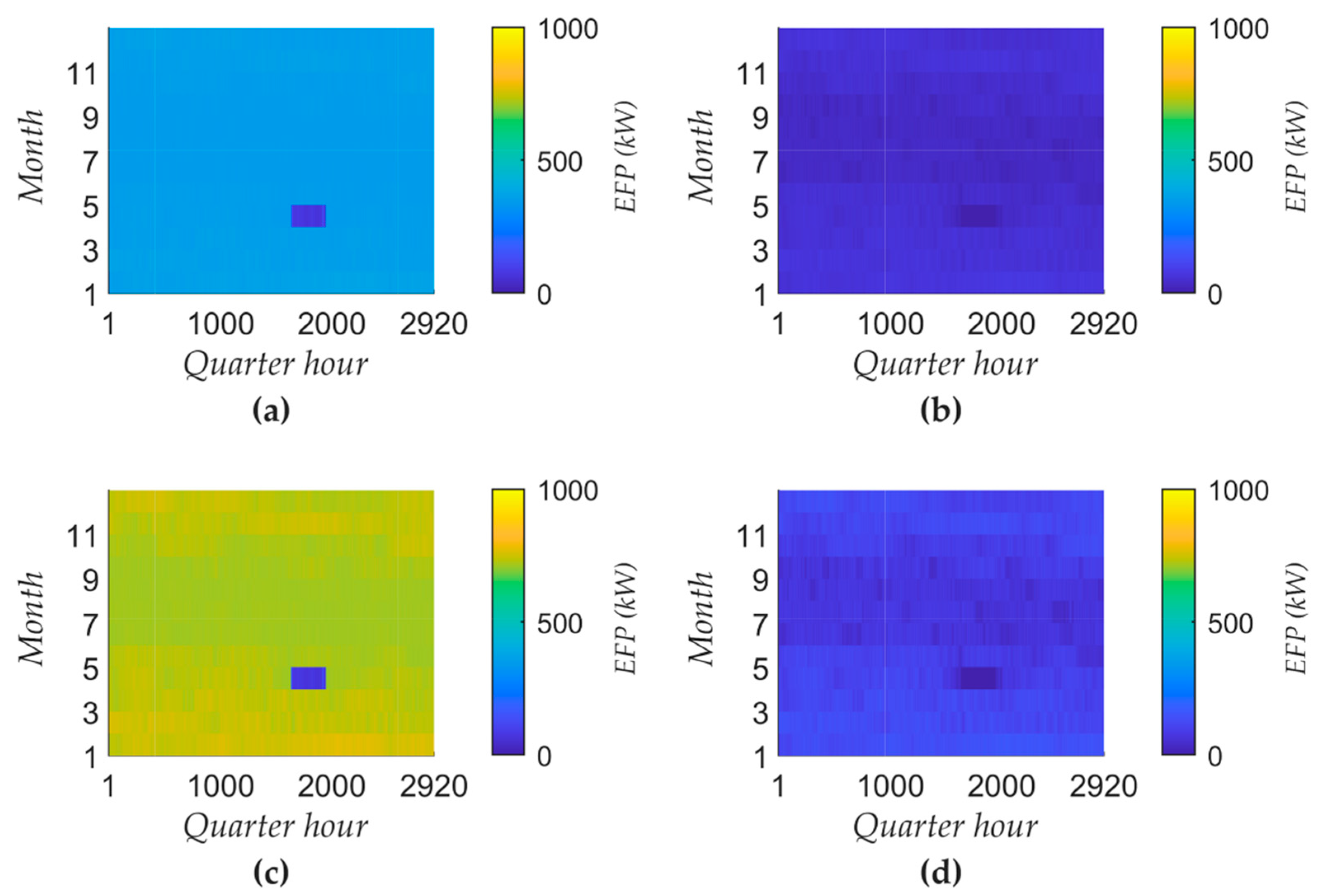
Figure 6 shows the technical energy-flexibility potential of the evaporator and the superheater for primary balancing power (PBP), negative secondary balancing power (SBP) and negative minutes’ balancing power (MBP). The annual average energy-flexibility potential of the total steam generation system is 3.1 MW for primary balancing power, 4.8 MW for negative secondary balancing power and 5.6 MW for negative minutes’ balancing power.
When positive balancing power is requested, meaning the electrical steam generator is switched off, no violation of the restrictions is observed, so the technical energy-flexibility potential corresponds to the theoretical one. The potential of positive secondary balancing power and minutes’ balancing power corresponds to the theoretical potential shown in
Figure 5 and amounts to an annual average of 6.1 MW. For marketing energy flexibility on the day-ahead market, it is assumed that there is sufficient time to control the devices in a way such that the technical potential corresponds to the theoretical one. Accordingly, the potential is equal to the theoretical negative secondary balancing power shown in
Figure 5.
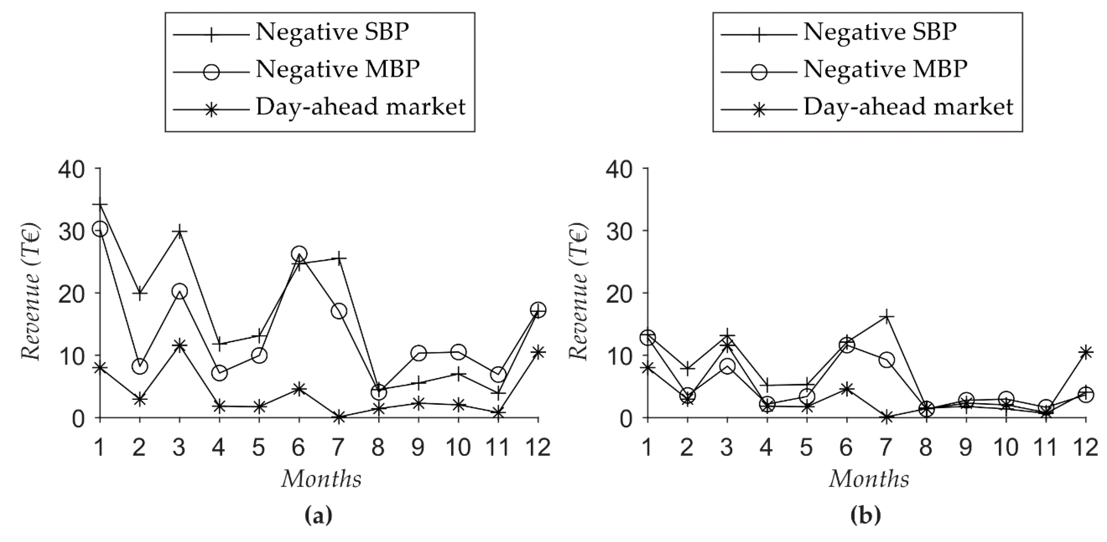
In addition to the technical potential, the economic potential is examined under the assumption of minimal taxes and levies. Despite this strict assumption, marketing positive balancing power does not lead to positive revenues because of the high electricity price required for reserving the potential. Therefore,
Figure 7 shows only the results for marketing negative balancing power as secondary and negative minutes’ balancing power and on the day-ahead market, which leads to positive revenues. To illustrate the relevance of the bidding strategy, the results for an optimal bidding strategy are shown on the left side and for a realistic bidding strategy on the right side. The variation of taxes only affects the day-ahead market since there are fewer points in time when the electricity price is lower than the gas price. Finally, there is no positive revenue for maximum taxes and charges.
5.2. Energy-Flexibility Potential via Inherent Energy Storage
In this section, the energy-flexibility potential enabled by the inherent storage capacity of the steam supply system is examined. Due to the quarter-hourly fluctuating total steam demand while operating with a single steam producer, it is not possible to meet the requirements for the holding period of secondary or minutes’ balancing power. Consequently, the energy-flexibility potential being marketed as primary balancing power and on the day-ahead market is investigated. As
Figure 8 shows, the energy-flexibility potential does not depend on the steam demand but only on the volume of the distribution network and the volume of the steam producer as well as the superheater. In April, no energy-flexibility potential is observed due to a production shutdown. The energy-flexibility potential for the day-ahead market amounts to 800 kW and is twice as high as it is for marketing primary balancing power because the potential does not have to be provided in both the positive and negative direction. Over 60% of the energy-flexibility potential results from the liquid water stored within the evaporator, since the evaporation temperature changes due to different evaporation pressures. Thus, the liquid water within the evaporator serves as an inherent sensible heat storage.
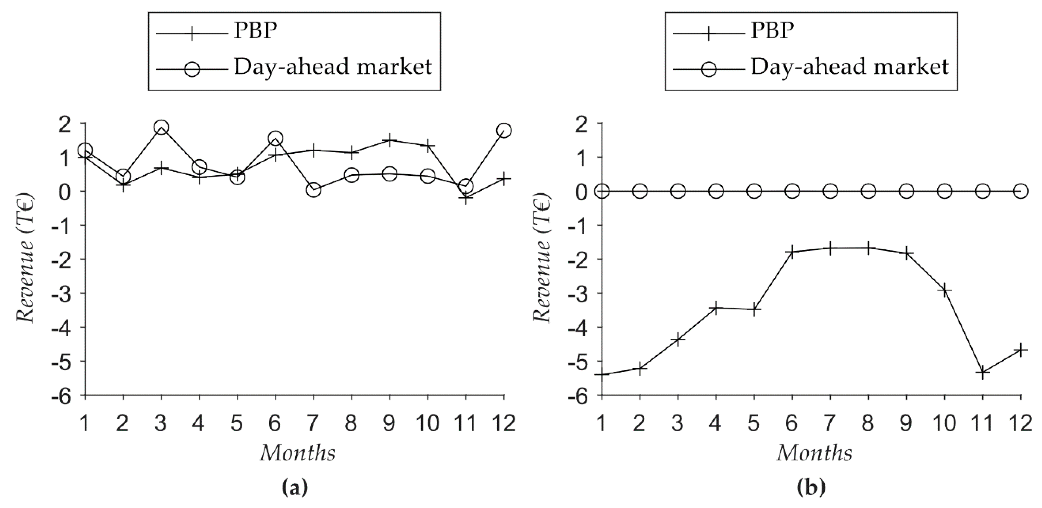
The economic potential is analyzed under the assumption of an optimal bidding strategy.
Figure 9 shows the revenues for minimum and maximum taxes. For maximum taxes there are no revenues at the day-ahead market because no points in time show a negative electricity price. Since marketing primary balancing power requires a higher pressure and temperature level, the higher electricity costs for reserving energy-flexibility potential in both directions cannot be covered.
5.3. Energy-Flexibility Potential via Process Parameter Adjustment
For this measure the network pressure and temperature are varied within the permitted limits, which influences the power consumption of the electric steam generator. As for storing energy inherently, this scenario assumes operating with a single steam generator, which is why
Figure 10 shows the energy-flexibility potential for only primary balancing power and the day-ahead market.
Due to almost pressure-independent evaporation enthalpy within the permissible pressure range,
Figure 10 shows a comparatively low energy-flexibility potential for the evaporator. The energy-flexibility potential of the superheater, which results from the changed temperature difference, is significantly higher. Due to the symmetrical flexibility offer, the marketable potential on the primary balancing power market is only half as large as it is on the day-ahead market. Since the energy-flexibility potential is significantly lower than for the other flexibility measures, no economic evaluation is carried out.
5.4. Interaction between Flexibilization and Energy Efficiency
The energy flexibilization of a system usually also influences its energy efficiency due to different generation technologies and operating parameters. As mentioned in
Section 3.4, evaluating the energy efficiency in detail requires a more accurate modeling approach of the steam consumers, so these results should be interpreted with particular respect to the influence of different energy-flexibility measures. Accordingly,
Figure 11 shows the changes in energy efficiency due to the different generation technologies as well as the variation of process parameters between the upper bound (UB) and lower bound (LB) for pressure and temperature. This shows that decreasing energy efficiency due to the increasing pressure and temperature, when requesting an energy-flexibility potential, is compensated by using an electrical steam generator, which has a higher energy efficiency than the gas-powered steam generator.
6. Discussion and Conclusions
This paper focuses on the evaluation of energy-flexibility measures for industrial steam supply systems by using dynamic simulation models. For this purpose, a practice-oriented method for the physical modeling of energy-relevant components and the simulation of energy-flexibility measures in steam supply systems is presented. Furthermore, measure-specific control strategies for the determination of the technical and economic energy-flexibility potential are derived. Finally, the method is applied to a representative steam supply system based on real data of the year 2019.
As with any simulation-based method, a compromise between model accuracy and parameterization effort must be made. For the presented approach, the aim is to develop a generalized and modular methodology to consider technical and economic aspects when evaluating energy-flexibility measures in industrial steam supply systems. For this purpose, physical simulation models of the energetically relevant components are developed, which allow the dynamic simulation of energy-flexibility measures. To be able to use the methodology in the early stages of design processes, great importance is given to the development of generic component models and their parameterization. Since the realization of energy-flexibility measures usually requires a strong data base of the regarded system, it is assumed that an energy management and monitoring system is already available. Thus, model parameterization can be performed using only standard data sheets and the data collected by the monitoring system. Due to the use of highly generic models, the methodology shown can be applied to steam supply systems of diverse system topologies.
The application of the presented methodology to the investigated steam supply system shows that industrial steam supply systems of this size show energy-flexibility potentials of up to 10 MW in the case of bivalent steam generation and up to 800 kW when using the system’s inherent storage capacity. In particular, in the case of bivalent steam generation, partial flexibilization could also be realized. Since industrial plants usually have redundancies in their energy supply, an electrical steam generator could be kept as a prospective redundancy, which could also be used for marketing flexibility. The economic evaluation shows that the profitability of energy-flexibility measures depends largely on the amount of tax and levies. In particular, the high share of fixed components in the electricity price often prevents marketing energy-flexibility potentials from being profitable. A change in pricing policy could lead to trading energy flexibility in the future. Finally, it should be noted that the profitability of energy-flexibility measures is highly dependent on the site location and the company, as large companies generally have very specific energy supply contracts.
The presented method offers various possibilities for further research projects. Within the research project SynErgie, further investigations will focus on the application of the method to water-based industrial supply systems. In addition, the method can be extended to include measures to make the heat consumption behavior more flexible. Regarding the economic evaluation, the consideration of energy prices for marketing secondary and minutes’ balancing power could be desirable in the future. Further research could also focus on detailing the simulation models, wherein a practical and user-friendly parameterization process should be considered. In particular, the steam generator model could be extended by a specific degasser model. Moreover, extending the methodology for application to steam supply systems with backpressure and extraction condensing steam turbines is desirable. This also requires detailing of the steam consumption model.
Finally, the automation of individual tasks, such as pre- and post-processing, as well as simulation studies within the framework of a planning tool could offer additional benefits for system planners of future steam supply systems.


