
iGREEN: An Integrated Emission Model for Mixed Bus Fleets

 ,
,  ,
,
Abstract
:1. Introduction
Rationale of the Paper
2. The Right Emission Model for the Right Bus Fleet
2.1. Emission Models: Features and Difficulties
The Problem of Obsolescence
3. A Methodology to Address the Obsolescence Issue
3.1. The iGREEN Development
- M1 ≤ 80,000 km;
- 80,000 km ≤ M2 ≤ 161,000 km;
- M3 > 161,000 km, thus coping with the COPERT’s limitation.
3.2. The Adopted Methodology
- in terms of stock configuration, iGREEN specifically deals with vehicles compliant with EURO standards, from II to VI. This facilitates operators when selecting this option; on the contrary, in the other models, the same task could be time-consuming, as operators have to identify the right stock configuration among large sets of vehicles with different technologies;
- even fewer input data than COPERT and much less than IVE to get a detailed calculation of emissions;
- iGREEN’s environmental variables are set to meet operators’ different requirements (assessment according to season, monthly or yearly basis) and operational situations (different types of slopes), whereas the other models rely just on average minimum and maximum temperature and humidity (COPERT), or altitude (IVE);
- Emissions are, therefore, calculated according to a larger set of operational features (being computed the temperatures, slopes and mileage), than in the other models.
- Design of an initial emission inventory database for EURO IV and EURO V engines based on the IVE one and its further integration with the COPERT’s one to include also inputs from buses with EURO VI engines. This resulted in the full iGREEN Emission Inventory Database (GEID);
- Development of bilinear regression functions to enable simplified calculations procedures (by a simple spreadsheet), from which the iGREEN algorithms for the maintenance software could be further implemented;
- Design of test features and selection of the case studies;
- Assessment of the case studies results for further refinement of the iGREEN procedures, if need be.
3.2.1. The Selection of the Case Studies
3.2.2. Specific Methodological Requirements
- average hourly speed;
- amount of engine ignitions;
- vehicle specific power—VSP;
- engine stress—ES;
- “bins”.
4. The Case Studies
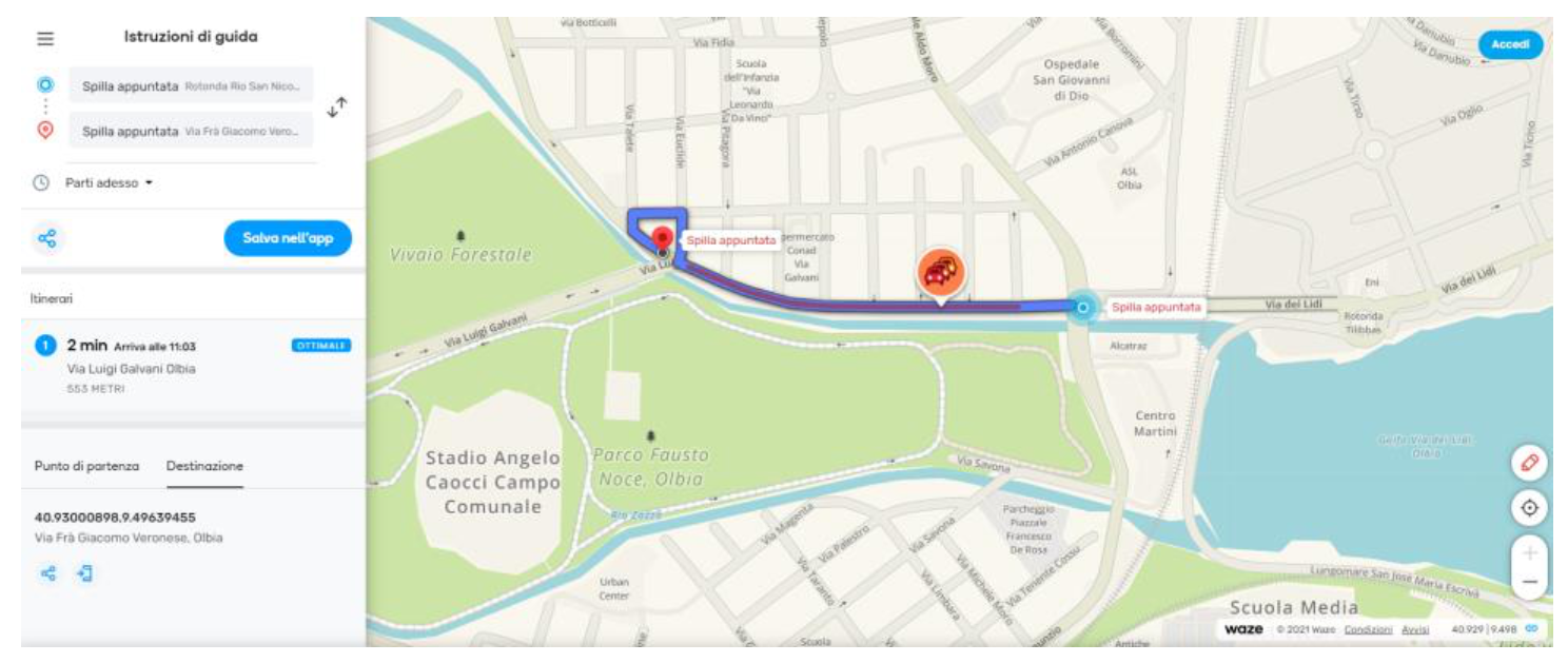
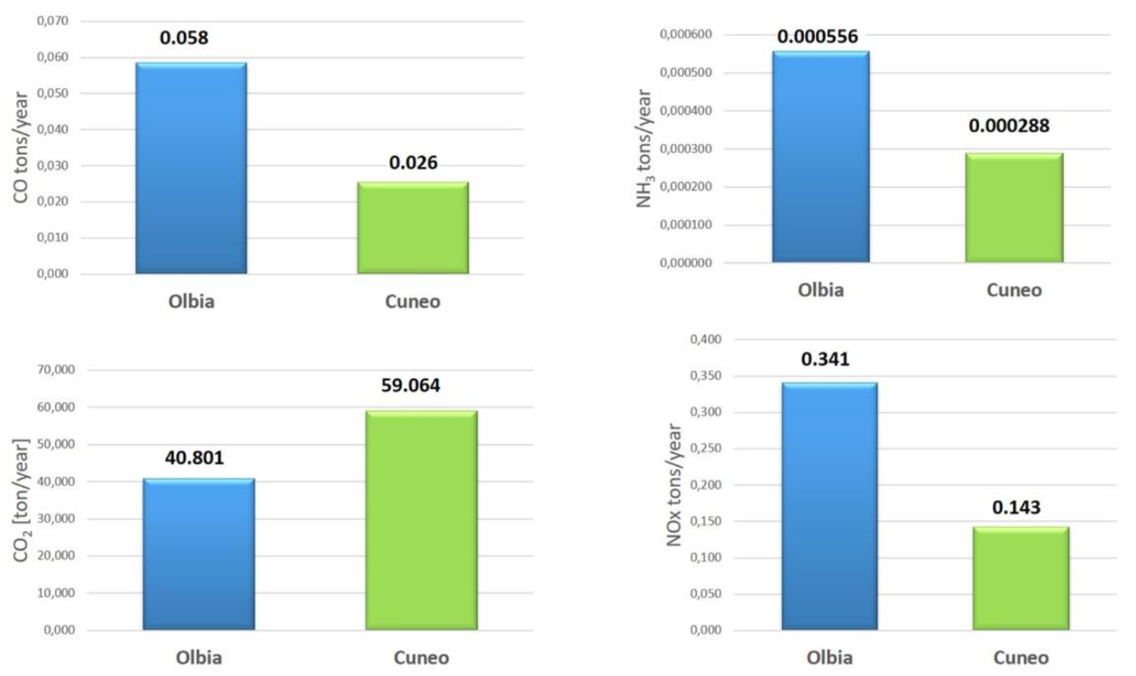
4.1. The Olbia Test
- driving cycles (short urban, long urban, and extra urban);
- speed ranges (12.5, 25, 30 km/h, respectively);
- hourly ignitions (2, 1, 0.5 events, respectively);
- weather conditions (air temperature: 20 °C, 25 °C, 30 °C);
- average road slope (grade: 0, 1, 2, 3%).
Creating the Software Interface for iGREEN
4.2. The Cuneo Test
5. The Results Achieved
5.1. Emissions Variation Trends
5.2. Cross-Case and Cross-Model Comparisons
5.3. Finalizing iGREEN
6. Discussion: Will the Environmental Concern Still Be a Priority?
7. Concluding Remarks
Author Contributions
Funding
Acknowledgments
Conflicts of Interest
References
- UITP. Global Bus Survey. May 2019. Available online: https://www.uitp.org/publications/global-bus-survey/ (accessed on 10 January 2020).
- Bloomberg NEF, Electric Vehicle Outlook 2020. Available online: https://about.bnef.com/electric-vehicle-outlook/ (accessed on 27 December 2020).
- Bousse, Y.; Corazza, M.V.; Arriaga, D.S.; Sessing, G. Electrification of public transport in Europe: Vision and practice from the ELIPTIC project. In Proceedings of the 2018 IEEE International Conference on Environment and Electrical Engineering and 2018 IEEE Industrial and Commercial Power Systems Europe (EEEIC/I&CPS Europe), Palermo, Italy, 12–15 June 2018; pp. 1–6. [Google Scholar] [CrossRef]
- Corazza, M.V.; Guida, U.; Musso, A.; Tozzi, M. From EBSF to EBSF_2: A compelling agenda for the bus of the future: A decade of research for more attractive and sustainable buses. In Proceedings of the 2016 IEEE 16th International Conference on Environment and Electrical Engineering (EEEIC), Florence, Italy, 7–10 June 2016; pp. 1–6. [Google Scholar] [CrossRef]
- ASSTRA. Investire nel TPL: Scenari e fabbisogni. February 2019. Available online: https://www.trasporti-italia.com/citta/convegno-nazionale-asstra-investire-nel-tpl-scenari-e-fabbisogni/37236 (accessed on 10 January 2020).
- Stempien, J.; Chan, S. Comparative study of fuel cell, battery and hybrid buses for renewable energy constrained areas. J. Power Sources 2017, 340, 347–355. [Google Scholar] [CrossRef]
- Meishner, F.; Sauer, D.U. Technical and economic comparison of different electric bus concepts based on actual demonstrations in European cities. IET Electr. Syst. Transp. 2020, 10, 144–153. [Google Scholar] [CrossRef]
- Santos, D.; Kokkinogenis, Z.; De Sousa, J.F.; Perrotta, D.; Rossetti, R.J.F. Towards the integration of electric buses in conventional bus fleets. In Proceedings of the 2016 IEEE 19th International Conference on Intelligent Transportation Systems (ITSC), Rio de Janeiro, Brazil, 1–4 November 2016; pp. 88–93. [Google Scholar] [CrossRef]
- Musso, A.; Corazza, M.V.; Information, R. Visioning the bus system of the future: Stakeholders’ perspective. Transp. Res. Rec. J. Transp. Res. Board 2015, 2533, 109–117. [Google Scholar] [CrossRef]
- Bektaş, T.; Laporte, G. The pollution-routing problem. Transp. Res. Part B Methodol. 2011, 45, 1232–1250. [Google Scholar] [CrossRef]
- Iris, Ç.; Lam JS, L. A review of energy efficiency in ports: Operational strategies, technologies and energy management systems. Renew. Sustain. Energy Rev. 2019, 112, 170–182. [Google Scholar] [CrossRef]
- Venturini, G.; Iris, Ç.; Kontovas, C.A.; Larsen, A. The multi-port berth allocation problem with speed optimization and emission considerations. Transp. Res. Part D Transp. Environ. 2017, 54, 142–159. [Google Scholar] [CrossRef] [Green Version]
- Zhang, X.; Lam JS, L.; Iris, Ç. Cold chain shipping mode choice with environmental and financial perspectives. Transp. Res. Part D Transp. Environ. 2020, 87, 102537. [Google Scholar] [CrossRef]
- Tsai, W.-H.; Lee, K.-C.; Liu, J.-Y.; Lin, H.-L.; Chou, Y.-W.; Lin, S.-J. A mixed activity-based costing decision model for green airline fleet planning under the constraints of the European Union Emissions Trading Scheme. Energy 2012, 39, 218–226. [Google Scholar] [CrossRef]
- Posada, F. CNG Bus Emissions Roadmap: From Euro III to Euro VI; International Council on Clean Transportation: Washington, DC, USA, 2009; p. 5. [Google Scholar]
- Nanaki, E.; Koroneos, C.; Roset, J.; Susca, T.; Christensen, T.; Hurtado, S.D.G.; Rybka, A.; Kopitovic, J.; Heidrich, O.; López-Jiménez, P.A. Environmental assessment of 9 European public bus transportation systems. Sustain. Cities Soc. 2017, 28, 42–52. [Google Scholar] [CrossRef]
- Li, F.; Zhuang, J.; Cheng, X.; Li, M.; Wang, J.; Yan, Z. Investigation and prediction of heavy-duty diesel passenger bus emissions in Hainan using a COPERT model. Atmosphere 2019, 10, 106. [Google Scholar] [CrossRef] [Green Version]
- Jimenez, F.B.P.; Román, A. Urban bus fleet-to-route assignment for pollutant emissions minimization. Transp. Res. Part E Logist. Transp. Rev. 2016, 85, 120–131. [Google Scholar] [CrossRef]
- Varella, R.A.; Giechaskiel, B.; Sousa, L.; Duarte, G. Comparison of portable emissions measurement systems (PEMS) with laboratory grade equipment. Appl. Sci. 2018, 8, 1633. [Google Scholar] [CrossRef] [Green Version]
- Giechaskiel, B.; Clairotte, M.; Valverde-Morales, V.; Bonnel, P.; Kregar, Z.; Franco, V.; Dilara, P. Framework for the assessment of PEMS (Portable Emissions Measurement Systems) uncertainty. Environ. Res. 2018, 166, 251–260. [Google Scholar] [CrossRef] [PubMed]
- Özener, O.; Özkan, M. Fuel consumption and emission evaluation of a rapid bus transport system at different operating conditions. Fuel 2020, 265, 117016. [Google Scholar] [CrossRef]
- Yu, H.; Liu, Y.; Li, J.; Liu, H.; Ma, K. Real-Road driving and fuel consumption characteristics of public buses in Southern China. Int. J. Automot. Technol. 2020, 21, 33–40. [Google Scholar] [CrossRef]
- Gómez, A.; Fernández-Yáñez, P.; Soriano, J.A.; Sánchez-Rodríguez, L.; Mata, C.; García-Contreras, R.; Armas, O.; Cárdenas, M.D. Comparison of real driving emissions from Euro VI buses with diesel and compressed natural gas fuels. Fuel 2021, 289, 119836. [Google Scholar] [CrossRef]
- Kozak, M.; Lijewski, P.; Fuc, P. Exhaust emissions from a city bus fuelled by oxygenated diesel fuel. SAE Tech. Pap. Ser. 2020. [Google Scholar] [CrossRef]
- Pan, Y.; Qiao, F.; Tang, K.; Chen, S.; Ukkusuri, S.V. Understanding and estimating the carbon dioxide emissions for urban buses at different road locations: A comparison between new-energy buses and conventional diesel buses. Sci. Total Environ. 2020, 703, 135533. [Google Scholar] [CrossRef] [PubMed]
- Rosero, F.; Fonseca, N.; López, J.-M.; Casanova, J. Real-world fuel efficiency and emissions from an urban diesel bus engine under transient operating conditions. Appl. Energy 2020, 261, 114442. [Google Scholar] [CrossRef]
- Franco, V.; Kousoulidou, M.; Muntean, M.; Ntziachristos, L. Road vehicle emission factors development: A review. Atmos. Environ. 2013, 70, 84–97. [Google Scholar] [CrossRef]
- Borge García, R.; Lumbreras Martin, J.; Perez Rodriguez, J.; Vedrenne, M.; Andres Almeida, J.M.; Rodriguez Hurtado, M.E. Development of road traffic emission inventories for urban air quality modeling in Madrid (Spain). In Proceedings of the 21st International Emission Inventory Conference Air Quality Challenges: Tackling the Changing Face of Emissions, San Diego, CA, USA, 13–16 April 2015; pp. 1–36. [Google Scholar]
- Linton, C.; Grant-Muller, S.; Gale, W.F. Approaches and techniques for modelling CO2 emissions from road transport. Transp. Rev. 2015, 35, 533–553. [Google Scholar] [CrossRef]
- Jaworski, A.; Mądziel, M.; Lejda, K. Creating an emission model based on portable emission measurement system for the purpose of a roundabout. Environ. Sci. Pollut. Res. 2019, 26, 21641–21654. [Google Scholar] [CrossRef] [Green Version]
- Alkafoury, A.; Bady, M.; Aly, M.H.F.; Negm, A.M. Emissions modeling for road transportation in urban areas: State-of-Art review. In Proceedings of the 23rd International Conference on “Environmental Protection is a Must”, Alexandria, Egypt, 11–13 May 2013; pp. 1–16. [Google Scholar]
- Boulter, P.G.; McCrae, I.S. ARTEMIS: Assessment and Reliability of Transport Emission Models and Inventory Systems—Final Report; TRL: London, UK, 2007. [Google Scholar]
- Boulter, P.G.; McCrae, I.S.; Barlow, T.J. A Review of Instantaneous Emission Models for Road Vehicles; TRL Limited: Wokingham, UK, 2007. [Google Scholar]
- Klein, J.; Geilenkirchen, G. Methods for calculating the emissions of transport in the Netherlands. Task Force on Transportation of the Dutch Pollutant Release and Transfer Register; TNO: Utrecht, The Netherlands, 2018. [Google Scholar]
- Guor, S.; Zhang, Y.; Cai, G.Q. Study on exhaust emission test of diesel vehicles based on PEMS. Procedia Comput. Sci. 2020, 166, 428–433. [Google Scholar] [CrossRef]
- Kliucininkas, L.; Matulevicius, J.; Martuzevicius, D. The life cycle assessment of alternative fuel chains for urban buses and trolleybuses. J. Environ. Manag. 2012, 99, 98–103. [Google Scholar] [CrossRef]
- Smit, R.; Kingston, P.; Tooker, R.; Neale, D.; Torr, S.; Harper, R.; O’Brien, E.; Harvest, D.; Wainwright, D. A Brisbane tunnel study to assess the accuracy of Australian motor vehicle emission models and examine the main factors affecting prediction errors. Air Qual. Clim. Chang. 2015, 49, 35–41. [Google Scholar]
- Emisia. COPERT 5 Manual; Microsoft Windows. Available online: https://copert.emisia.com/manual/ (accessed on 5 December 2019).
- Boulter, P.G. Emission Factors 2009: Report 6—Deterioration Factors and Other Modelling Assumption on Road Vehicles; TRL: London, UK, 2009. [Google Scholar]
- NAEI—National Atmospheric Emission Inventory. Method for Applying Emission Degradation Correction Factors for the COPERT 4 Nox for Light Duty Petrol Vehicles; Department for Business, Energy and Industrial Strategy: London, UK, 2012. [Google Scholar]
- Carbone, D.; Proia, E. (Eds.) EBSF Deliverable—Report on the Energy Efficiency of Bus System; ASSTRA: Rome, Italy, 2013; restricted document, unpublished. [Google Scholar]
- EUROSTAT, E.U. Transport in Figures—Statistical Pocketbook 2020; Publications Office of the European Union: Luxembourg, 2020. [Google Scholar]
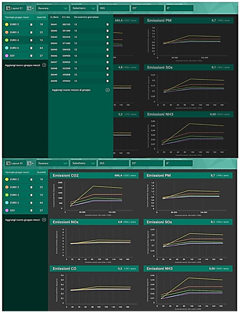
- Corazza, M.V.; Magnalardo, S.; Musso, A.; Petracci, E.; Tozzi, M.; Vasari, D.; De Verdalle, E. Testing an innovative predictive management system for bus fleets: Outcomes from the Ravenna case study. IET Intell. Transp. Syst. 2018, 12, 286–293. [Google Scholar] [CrossRef]
- Lents, J.; Davis, N. IVE Model User’s Guide, Model and Data Files. Technical Report; US Environmental Protection Agency: Washington, DC, USA, 2009; Available online: http://www.issrc.org (accessed on 16 December 2018).
- Guo, H.; Zhang, Q.-Y.; Shi, Y.; Wang, D.-H. Evaluation of the International Vehicle Emission (IVE) model with on-road remote sensing measurements. J. Environ. Sci. 2007, 19, 818–826. [Google Scholar] [CrossRef]
- Davis, N.; Lents, J.; Osses, M.; Nikkila, N.; Barth, M. Development and application of an international vehicle emissions model. Transp. Res. Rec. J. Transp. Res. Board 2005, 1939, 156–165. [Google Scholar] [CrossRef]
- Nagpure, A.S.; Gurjar, B. Development and evaluation of vehicular air pollution inventory model. Atmos. Environ. 2012, 59, 160–169. [Google Scholar] [CrossRef]
- Ghadiri, Z.; Rashidi, Y.; Broomandi, P. Evaluation Euro IV of effectiveness in transportation systems of Tehran on air quality: Application of IVE model. Pollution 2017, 3, 639–653. [Google Scholar]
- Hongzhao, D.O.; Yongbin, X.U.; Ning, C. A research on the vehicle emission factors of real world driving cycle in Hangzhou city based on IVE model. Automot. Eng. 2011, 33, 1034–1038. [Google Scholar]
- ISSRC. IVE Model Users Manual, Version 2; International Sustainable Systems Research Center—ISSRC: La Habra, CA, USA, 2008; Available online: http://issrc.org/ive/downloads/manuals/UsersManual.pdf (accessed on 5 March 2018).
- Musso, A.; Corazza, M.V.; Tozzi, M. Car sharing in Rome: A case study to support sustainable mobility. Procedia Soc. Behav. Sci. 2012, 48, 3482–3491. [Google Scholar] [CrossRef] [Green Version]
- Corazza, M.V.; Musso, A.; Finikopoulos, K.; Sgarra, V. An analysis on health care costs due to accidents involving powered two wheelers to increase road safety. Transp. Res. Procedia 2016, 14, 323–332. [Google Scholar] [CrossRef] [Green Version]
- Sgarra, V.; Di Mascio, P.; Corazza, M.V.; Musso, A. An application of ITS devices for powered two-wheelers safety analysis: The Rome case study. Adv. Transp. Stud. 2014, 33, 85–96. [Google Scholar]
- Fauser, P.; Thomsen, M.; Pistocchi, A.; Sanderson, H. Using multiple regression in estimating (semi) VOC emissions and con-centrations at the European scale. Atmos. Pollut. Res. 2010, 1, 132–140. [Google Scholar] [CrossRef] [Green Version]
- van de Kassteele, J.; Koelemeijer, R.B.A.; Dekkers, A.L.M.; Schaap, M.; Homan, C.D.; Stein, A. Statistical mapping of PM10 concentrations over Western Europe using secondary information from disper-sion modeling and MODIS satellite observations. Stoch. Environ. Res. Risk Assess. 2006, 21, 183–194. [Google Scholar] [CrossRef]
- Xu, H.; Bechle, M.J.; Wang, M.; Szpiro, A.A.; Vedal, S.; Bai, Y.; Marshall, J.D. National PM2.5 and NO2 exposure models for China based on land use regression, satellite measurements, and universal kriging. Sci. Total. Environ. 2019, 655, 423–433. [Google Scholar] [CrossRef] [Green Version]
- Jiménez-Palacios, J.L. Understanding and Quantifying Motor Vehicle Emissions with Vehicle Specific Power and TILDAS Remote Sensing. Ph.D. Thesis, Massachusetts Institute of Technology, Department of Mechanical Engineering, Cambridge, MA, USA, February 1999. [Google Scholar]
- Zhai, H.; Frey, C.; Nagui, M.A. Vehicle-Specific power approach to speed-and facility-specific emissions estimates for diesel transit buses. Environ. Sci. Technol. 2008, 42, 7985–7991. [Google Scholar] [CrossRef] [PubMed]
- Liao, R.; Chen, X.; Yu, L.; Sun, X. Analysis of emission effects related to drivers’ compliance rates for cooperative vehicle-infrastructure system at signalized intersections. Int. J. Environ. Res. Public Health 2018, 15, 122. [Google Scholar] [CrossRef] [PubMed] [Green Version]
- Onchang, R.; Noisopa, K.; Pawarmart, I. Changes of air pollution and climate forcing emissions due to fuel switching to gasohol in motorcycle fleet in an urban area of Thailand. Environ. Asia 2017, 10, 94–104. [Google Scholar] [CrossRef]
- Lai, J.; Yu, L.; Song, G.; Guo, P.; Chen, X. Development of city-specific driving cycles for transit buses based on VSP distributions: Case of Beijing. J. Transp. Eng. 2013, 139, 749–757. [Google Scholar] [CrossRef]
- Lozhkina, O.V.; Lozhkin, V.N. Estimation of nitrogen oxides emissions from petrol and diesel passenger cars by means of on-board monitoring: Effect of vehicle speed, vehicle technology, engine type on emission rates. Transp. Res. Part D Transp. Environ. 2016, 47, 251–264. [Google Scholar] [CrossRef]
- Seigneur, C. Emissions of Air Pollutants and Emission Control Technologies; Cambridge University Press: Cambridge, UK, 2019. [Google Scholar]
- Cooper, B. Sulphate emissions from automobile exhaust. Platin. Met. Rev. 1976, 20, 38–45. [Google Scholar]
- El-Baza, F.K.; Gadb, M.S.; Abdoc, S.M.; Abedd, K.A.; Mattere, I.A. Performance and exhaust emissions of a diesel engine burning algal biodiesel blends. Int. J. Mech. Mechatron. Eng. 2016, 16, 151–158. [Google Scholar]
- Muhammad, S.; Long, X.; Salman, M. COVID-19 pandemic and environmental pollution: A blessing in disguise? Sci. Total. Environ. 2020, 728, 138820. [Google Scholar] [CrossRef] [PubMed]
- Le Quéré, C.; Jackson, R.B.; Jones, M.W.; Smith, A.J.P.; Abernethy, S.; Andrew, R.M.; De Gol, A.J.; Willis, D.R.; Shan, Y.; Canadell, J.G.; et al. Temporary reduction in daily global CO2 emissions during the COVID-19 forced confinement. Nat. Clim. Chang. 2020, 3, 1–8. [Google Scholar] [CrossRef]
- Corazza, M.V.; Musso, A. Urban transport policies in the time of pandemic, and after: An arduous research agenda. Transp. Policy 2021, 103, 31–44. [Google Scholar] [CrossRef]
- Beyer, R.M.; Manica, A.; Mora, C. Shifts in global bat diversity suggest a possible role of climate change in the emergence of SARS-CoV-1 and SARS-CoV-2. Sci. Total Environ. 2021, 145413. [Google Scholar] [CrossRef]
- Sun, Z.; Wang, C.; Ye, Z.; Bi, H. Long short-term memory network-based emission models for conventional and new energy buses. Int. J. Sustain. Transp. 2021, 15, 229–238. [Google Scholar] [CrossRef]


| COPERT | IVE | |
|---|---|---|
| Input Variables | ||
| Environmental information | Annual average minimum and maximum temperature (C°), humidity (%) | Altitude (m) |
| Fuel specifications | Energy content (MJ/kg), H:C ratio, O:C ratio, Density, S, Pb, Cd, Cu, Cr, Ni, Se, Zn, Hg, As | Gasoline (fuel quality, S, Pb, Benzene, % Oxygenate), diesel (fuel quality, S) |
| Lubricant specifications | S, Pb, Cd, Cu, Cr, Ni, Se, Zn, Hg, As, H:C ratio, O:C ratio | No specifications |
| Stock configuration | 448 different vehicles with different technologies available | 1372 different vehicles with different technologies available |
| Stock data per vehicle per technology | Annual mean activity (km); lifetime cumulative activity (km); | Distance (km) and average speed (km/h) in the hour evaluated. Acceleration, deceleration and grade of slope, second-by-second |
| Circulation mode per vehicle, technology | Emission factors defined by % in rural, urban or highway and their average speed in each mode (km/h) | Emission factors using the VSP and engine stress calculated by the user and the table of BINs |
| Emission calculation method | Vehicle activity × emission factor | Vehicle activity disaggregated by specific mode × emission factor |
| Outputs | ||
| Types of emissions | Hot and cold emissions | Running and start-up |
| Estimated pollutant packages | 25 pollutants, including GHG (CO2, CH4, N2O) | 15 pollutants, including GHG (CO2, CH4, N2O) |
| Default output units | tons/year | kg/h; kg/day |
| Advantages and Disadvantages | ||
| Advantages | Few input data to get a detailed emission calculation Input information on kilometers travelled and average speed is relatively easy to obtain from traffic models or field measurements. Large list of exhaust and nonexhaust pollutants Large amount of data from the driving conditions not needed | It has a large library of vehicles and technologies Emission factors are differentiated for various traffic conditions and driving patterns (VSP and BIN, further elaborated) It can get a detailed behavior of the emission during a single run |
| Disadvantages | Mileage degradation is not available for all the vehicles and all technologies | It does not consider the effect of the lubricant Data may not be easy to get without GPS It does not include Euro VI standard |
| iGREEN | |
|---|---|
| Input Variables | |
| Environmental information | Three different average and significant temperatures (20, 25 and 30 °C), these could be adaptable to the users’ requirement, i.e., season average, monthly average, yearly average; different types of slope |
| Fuel specifications | Gasoline (fuel quality, S, Pb, Benzene, % Oxygenate), diesel (fuel quality, S) |
| Lubricant specifications | No specifications |
| Stock configuration | Vehicles compliant with EURO standards from II to VI |
| Stock data per vehicle per technology | Annual mean activity (km); mileage (km) |
| Circulation mode per vehicle, technology | Emission factors defined by operations in urban (long or short) or extra urban cycles, with a large set of variables describing speed (km/h) and amount of engine ignitions (events/h) |
| Emission calculation method | Vehicle activity × emission factor (given by temperature, road slope and mileage) |
| Outputs | |
| Types of emissions | Running and start-up |
| Estimated pollutant package | CO2, NOx, CO, PM, SOx, NH3 |
| Default output units | tons/year |
| Advantages and Disadvantages | |
| Advantages | Few and simple input data to get a detailed emission calculation Fit to be easily used by EURO standard bus fleets It considers the mileage information, or the age of the vehicles measured in km Outcomes clearly revealing pollution levels |
| Disadvantages | Limited to the EURO technology It does not consider temperature higher than 30 °C |
| Cycle | Temp | Slope | Mileage | Max. Emission | Until 80k km: Linear Model | Over 80k km: Max. Emissions | |||
|---|---|---|---|---|---|---|---|---|---|
| M1 | M2 | M3 | Equation (1) | Equation (2) | |||||
| Urban Short | 20 °C | 0° | 621.49 | 1716.27 | 1770.32 | 1770.32 | 14.360 | 621.490 | 1770.32 |
| 1° | 642.79 | 1765.25 | 1753.27 | 1765.25 | 14.031 | 642.790 | 1765.25 | ||
| 2° | 660.28 | 1814.02 | 1805.7 | 1814.02 | 14.422 | 660.280 | 1814.02 | ||
| 3° | 678.09 | 1862.75 | 1850.11 | 1862.75 | 14.808 | 678.090 | 1862.75 | ||
| 25 °C | 0° | 677.03 | 1885.87 | 1873.03 | 1885.87 | 15.111 | 677.030 | 1885.87 | |
| 1° | 702.28 | 1959.85 | 1943.56 | 1959.85 | 15.720 | 702.280 | 1959.85 | ||
| 2° | 720.81 | 2009.85 | 1996.21 | 2009.85 | 16.113 | 720.810 | 2009.85 | ||
| 3° | 739.64 | 2062.81 | 2048.8 | 2062.81 | 16.540 | 739.640 | 2062.81 | ||
| 30 °C | 0° | 722.04 | 2010.46 | 1998.48 | 2010.46 | 16.105 | 722.040 | 2010.46 | |
| 1° | 737.97 | 2063.45 | 2049.48 | 2063.45 | 16.569 | 737.970 | 2063.45 | ||
| 2° | 757.33 | 2116.46 | 2102.09 | 2116.46 | 16.989 | 757.330 | 2116.46 | ||
| 3° | 776.3 | 2169.4 | 2154.69 | 2169.4 | 17.414 | 776.300 | 2169.4 | ||
| Urban Long | 20 °C | 0° | 481.47 | 1321.41 | 1312.34 | 1321.41 | 10.499 | 481.470 | 1321.41 |
| 1° | 509.61 | 1396.47 | 1386.98 | 1396.47 | 11.086 | 509.610 | 1396.47 | ||
| 2° | 536.41 | 1471.58 | 1461.59 | 1471.58 | 11.690 | 536.410 | 1471.58 | ||
| 3° | 563.07 | 1546.64 | 1536.22 | 1546.64 | 12.295 | 563.070 | 1546.64 | ||
| 25 °C | 0° | 488.16 | 1348.86 | 1339.72 | 1348.86 | 10.759 | 488.160 | 1348.86 | |
| 1° | 514.54 | 1423.99 | 1414.32 | 1423.99 | 11.368 | 514.540 | 1423.99 | ||
| 2° | 541.63 | 1499.13 | 1496 | 1499.13 | 11.969 | 541.630 | 1499.13 | ||
| 3° | 569.11 | 1574.17 | 1563.51 | 1574.17 | 12.563 | 569.110 | 1574.17 | ||
| 30 °C | 0° | 512.29 | 1418.75 | 1409.13 | 1418.75 | 11.331 | 512.290 | 1418.75 | |
| 1° | 540.2 | 1493.89 | 1483.76 | 1493.89 | 11.921 | 540.200 | 1493.89 | ||
| 2° | 568.3 | 1569.02 | 1558.38 | 1569.02 | 12.509 | 568.300 | 1569.02 | ||
| 3° | 593.94 | 1640.09 | 1632.96 | 1640.09 | 13.077 | 593.940 | 1640.09 | ||
| Extra Urban | 20 °C | 0° | 553.49 | 1479.61 | 1478.59 | 1479.61 | 11.577 | 553.490 | 1479.61 |
| 1° | 591.38 | 1580.68 | 1569.96 | 1580.68 | 12.366 | 591.380 | 1580.68 | ||
| 2° | 629.25 | 1681.71 | 1670.34 | 1681.71 | 13.156 | 629.250 | 1681.71 | ||
| 3° | 667.17 | 1782.81 | 1770.62 | 1782.81 | 13.946 | 667.170 | 1782.81 | ||
| 25 °C | 0° | 551.69 | 1508.13 | 1517.92 | 1517.92 | 12.078 | 551.690 | 1517.92 | |
| 1° | 589.75 | 1609.21 | 1598.29 | 1609.21 | 12.743 | 589.750 | 1609.21 | ||
| 2° | 626.54 | 1710.27 | 1698.66 | 1710.27 | 13.547 | 626.540 | 1710.27 | ||
| 3° | 663.49 | 1811.25 | 1798.97 | 1811.25 | 14.347 | 663.490 | 1811.25 | ||
| 30 °C | 0° | 580.6 | 1584.57 | 1573.8 | 1584.57 | 12.550 | 580.600 | 1584.57 | |
| 1° | 618.42 | 1685.66 | 1664 | 1685.66 | 13.341 | 618.420 | 1685.66 | ||
| 2° | 654.59 | 1786.7 | 1774.57 | 1786.7 | 14.151 | 654.590 | 1786.7 | ||
| 3° | 693.45 | 1887.66 | 1874.84 | 1887.66 | 14.928 | 693.450 | 1887.66 | ||
| Main Validation Data | Value | Unit |
|---|---|---|
| Operational Input Parameters | ||
| Mean activity (as annual average) | 60,000 | km |
| Life cumulative activity (sum of annual averages) | 300,000 | km |
| Share—urban peak | 15 | % |
| Share—urban off peak | 85 | % |
| Speed—urban peak | 15 | km/h |
| Speed—urban off peak | 25 | km/h |
| Fuel Input Parameters | ||
| Energy content | 42.6950 | MJ/kg |
| H:C ratio | 1.86 | |
| O:C ratio | 0 | |
| Density | 840 | kg/m3 |
| EURO IV | EURO V | |||
|---|---|---|---|---|
| M1 (<80 K km) | ||||
| Pollutant Emitted (t/year) | IVE | COPERT | IVE | COPERT |
| CO2 | 21.850 | 59.094 | 21.850 | 53.394 |
| NOx | 0.3587 | 0.3777 | 0.2044 | 0.4224 |
| CO | 0.0128 | 0.0776 | 0.0128 | 0.1348 |
| NH3 | 0.0012 | 0.0002 | 0.00126 | 0.00066 |
| M2 (80–160 K km) | ||||
| Pollutant Emitted (t/year) | IVE | COPERT | IVE | COPERT |
| CO2 | 54.192 | 59.094 | 54.1926 | 53.3945 |
| NOx | 0.3636 | 0.3777 | 0.2072 | 0.4224 |
| CO | 0.0134 | 0.0776 | 0.01349 | 0.1348 |
| NH3 | 0.0012 | 0.0002 | 0.00126 | 0.00066 |
| M3 (>160 K km) | ||||
| Pollutant Emitted (t/year) | IVE | COPERT | IVE | COPERT |
| CO2 | 53.823 | 59.094 | 53.823 | 53.3945 |
| NOx | 0.3710 | 0.3777 | 0.2115 | 0.4224 |
| CO | 0.0144 | 0.0776 | 0.0144 | 0.1348 |
| NH3 | 0.0012 | 0.0002 | 0.00126 | 0.00066 |
| Veh ID | Max Grade (m) | Operation Time (hh:mm) | Ignitions (Event/Day) | Avg. Speed Peak Hour (km/h) | Avg. Speed Off-Peak (km/h) | Peak Time Duration (hh:mm) |
|---|---|---|---|---|---|---|
| 1051 | 10 | 17:20 | 38 | 25 | 30 | 3:15 |
| 1052 | 65 | 12:10 | 12 | 31 | 38 | 3:23 |
| 1053 | 50 | 11:15 | 15 | 20 | 26 | 2:31 |
Publisher’s Note: MDPI stays neutral with regard to jurisdictional claims in published maps and institutional affiliations. |
© 2021 by the authors. Licensee MDPI, Basel, Switzerland. This article is an open access article distributed under the terms and conditions of the Creative Commons Attribution (CC BY) license (http://creativecommons.org/licenses/by/4.0/).
Share and Cite
Corazza, M.V.; Lizana, P.C.; Pascucci, M.; Petracci, E.; Vasari, D. iGREEN: An Integrated Emission Model for Mixed Bus Fleets. Energies 2021, 14, 1521. https://doi.org/10.3390/en14061521
Corazza MV, Lizana PC, Pascucci M, Petracci E, Vasari D. iGREEN: An Integrated Emission Model for Mixed Bus Fleets. Energies. 2021; 14(6):1521. https://doi.org/10.3390/en14061521
Chicago/Turabian StyleCorazza, Maria Vittoria, Paulo Cantillano Lizana, Marco Pascucci, Enrico Petracci, and Daniela Vasari. 2021. "iGREEN: An Integrated Emission Model for Mixed Bus Fleets" Energies 14, no. 6: 1521. https://doi.org/10.3390/en14061521