Article

Optimization of Flow Rate and Pipe Rotation Speed Considering Effective Cuttings Transport Using Data-Driven Models

1
Department of Petroleum Engineering, The University of Tulsa, Tulsa, OK 74104, USA
2
Department of Computer Engineering, TOBB University of Economics and Technology, 06560 Ankara, Turkey
3
Department of Mechanical Engineering, The University of Texas at Austin, Austin, TX 78712, USA
*
Author to whom correspondence should be addressed.
Energies 2021, 14(5), 1484; https://doi.org/10.3390/en14051484
Submission received: 3 February 2021 / Revised: 1 March 2021 / Accepted: 3 March 2021 / Published: 9 March 2021
(This article belongs to the Special Issue Recent Advances in Petroleum Drilling Engineering)

Abstract

:
Effectively transporting drilled cuttings to the surface is a vital part of the well construction process. Usually, mechanistic models are used to estimate the cuttings concentration during drilling. Based on the results from these model, operational parameters are adjusted to mitigate any nonproductive time events such as pack-off or lost circulation. However, these models do not capture the underlying complex physics completely and frequently require updating the input parameters, which is usually performed manually. To address this, in this study, a data-driven modeling approach is taken and evaluated together with widely used mechanistic models. Artificial neural networks are selected after several trials. The experimental data collected at The University of Tulsa–Drilling Research Projects (in the last 40 years) are used to train and validate the model, which includes a wide range of wellbore and pipe sizes, inclinations, rate-of-penetration values, pipe rotation speeds, flow rates, and fluid and cuttings properties. It is observed that, in many cases, the data-driven model significantly outperforms the mechanistic models, which provides a very promising direction for real-time drilling optimization and automation. After the neural network is proven to work effectively, an optimization attempt to estimate flow rate and pipe rotation speed is introduced using a genetic algorithm. The decision is made considering minimizing the required total energy for this process. This approach may be used as a design tool to identify the required flow rate and pipe rotation speed to acquire effective hole cleaning while consuming minimal energy.

Graphical Abstract

1. Introduction

In recent years, the energy industry has showed significant interest in the digitization of well construction processes for improved safety and cost reduction. To achieve that, robust and accurate modeling of physical processes is essential, and especially modeling cuttings transport is important to safely and successfully drill wells.
Most commonly, mechanistic models are used to estimate the cuttings concentration in wellbores. These models are used during the design and execution phases of operations. Based on the simulation results from the mechanistic model, several decisions can be made to alleviate potential hole cleaning problems. For example, the pump’s flow rate and the drill string’s rotation speed can be adjusted to mitigate nonproductive time (NPT) events. An NPT event can be a pack-off leading to a stuck pipe due to elevated cuttings accumulation around the bottomhole assembly (BHA), or it can be induced lost circulation due to elevated equivalent circulating density (ECD) in the presence of high concentrations of cuttings. Lost circulation can easily transform into a catastrophic blowout event. Therefore, it is important to model and monitor the cuttings concentration in the wellbore.
Up until now, these mechanistic models were useful; however, there are some inherent shortcomings to these models. First, a mechanistic model can be inaccurate because it is unlikely to perfectly model the complex physical interactions associated with cuttings transport. These include the effects of pipe rotation, eccentricity, inclination, chemical interactions, fluid and cuttings properties, etc. Additionally, mechanistic models frequently require updating the input parameters. Some of these parameters, such as geometry, trajectory, and fluid properties, may be extracted from daily drilling reports. However, there are a lot of manual measurement steps required to collect these inputs and a human operator is needed to input and maintain the model parameters [1]. This manual process is a major challenge that prevents streamlining well construction operations.
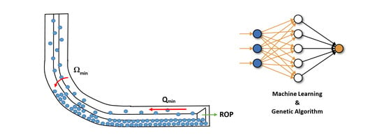
In this study, an alternative, data-driven modeling approach is taken with the aim to overcome the shortcomings of mechanistic models. After various trials, an artificial neural network model is used. The model is applied to the experimental datasets collected at The University of Tulsa—Drilling Research Projects (TUDRP). These datasets were collected through the experimental research projects conducted in the last 40 years, which include a wide spectrum of wellbore and pipe sizes, inclinations, rate-of-penetration (ROP) values, pipe rotation speeds, flow rates, and fluid and cuttings properties. The performance of the proposed model is compared with existing mechanistic models by comparing the results with the experimental datasets. The results show that, especially for this particular research area, the data-driven model performs significantly better. Finally, using this model, a genetic algorithm is applied to determine the optimal flow rate and pipe rotation speed. The decision is made considering the minimum required energy for this process.
Data-driven models are more practical to implement and show the potential to overcome the disadvantages of the mechanistic model by providing better accuracy and requiring fewer manual inputs. Therefore, data-driven models can be a better candidate in the act of digitizing the well construction process. In addition, to the best of the authors’ recollection, there is no optimization attempt reported in the literature regarding flow rate and rotation speed considering cuttings transport performance based on a quantitative function defined to be minimized using a machine learning technique.
The paper structure is organized as follows: After this brief introduction, existing relevant studies in the literature are presented in the Literature Review section along with machine learning and genetic algorithm-related topics. The results are analyzed and discussed in the Results and Discussions section. Finally, the conclusions are provided in the last section. In the Appendix, basic working structures of neural networks and genetic algorithms are introduced along with the particular network parameters used in the study.

2. Literature Review

Mechanistic and computational fluid dynamics (CFD) models for cuttings transport are very important because there is no direct measurement of cuttings deposition during drilling wells. The cuttings deposition is usually inferred by interpreting a multitude of sensory measurements (i.e., standpipe pressure, hook load, etc.), which are prone to human error. Therefore, the operations need to rely on simulations from these models. However, there is only a limited amount of literature, especially about data-driven models for cuttings transport. In this section, some literature about various modeling approaches for cuttings transport is presented.
Cayeux et al. [2] proposed a real-time, transient cuttings transport model that can calculate the distribution of cuttings along the wellbore. They applied this model to datasets that are from actual drilling operations and demonstrated the model’s usability cases with these two case studies. A good match between the surface measurements, observations, and model’s prediction was attained.
Erge and van Oort [3] introduced a new cuttings transport modeling approach including the effects of rotation and eccentricity. The proposed model was developed by constructing 3D velocity profiles and by comparing the local velocities to a local critical velocity definition to estimate the cuttings deposition along the trajectory of the wellbore. Then, they introduced time-dependency into the proposed model and demonstrated the model’s capabilities using an actual drilling dataset with a stuck pipe event that occurred due to cuttings pack-off. The results showed fair agreement between the model’s prediction and the data [4,5].
Ozbayoglu et al. [6] conducted a comparative analysis using physics-based and data-driven models for estimating the frictional pressure losses in an annulus. The results showed that the data-driven model more accurately captured the complex dynamics especially while the drill string was compressed and rotating.
Ozbayoglu et al. [7] developed a new cuttings-transport mechanistic model that includes the effects of drill-pipe rotation and eccentricity. The model can estimate the volumetric distribution phases in three-phase flow and the pressure losses in the horizontal sections. Additionally, they conducted experiments involving three-phase flow and compared the results from the mechanistic model to the experimental data. They noted a good agreement between them.
Ozbayoglu et al. [8] conducted cuttings transport experiments for a wide range of flow rates, cuttings injection rates, and inner pipe rotation speeds. Additionally, they recorded these experiments via a high-speed digital camera. They implemented an image processing algorithm to extract some characteristic information about cuttings transport during these experiments, such as the concentration of moving particles, their relative transport velocities, etc. These parameters were used as inputs to the mechanistic model and, in doing so, the performance of the mechanistic model improved significantly.
Tombul et al. [9] applied several data-driven models (linear and nonlinear regression, support vector regression (SVR), support vector machine (SVM), and artificial neural networks (ANN)) to predict the velocity and direction of the cuttings using experimental data collected via a particle image velocimeter. The experimental test matrix included a distinct rate of penetration values, inclinations, rotation speeds, and flow rates. They noted that SVM performed better when estimating the direction of the cuttings and that SVR better predicted velocity.
Zamora et al. [10] and, later, Friedheim and Contreras [11] presented a cuttings transport model that combines an analytical model, a fuzzy logic technique, and experimental data. The results of their model were presented under four categories ranging from “very good” to “poor” hole cleaning. They stated that this type of data-driven modeling is well suited for implementation and use during real-time operations, which is also verified in this present study.
Aggwu et al. [12] presented a comprehensive literature review of experimental, numerical, and artificial intelligence (AI) modeling studies on cuttings settling velocity research. They concluded that AI techniques provide a unique way to model the cuttings settling velocity and that a variety should be investigated to determine the most relevant technique for this field of research. In a more recent study, Aggwu et al. [13] applied ANN to estimate the cuttings settling velocity considering the cuttings shape, size, and density and the drilling fluid’s viscosity and density. They mentioned that, generally, physics-based models assume cuttings shape to be a perfect sphere. This assumption causes the model to be inaccurate in actual conditions. In contrast, they demonstrated that the ANN model can capture the effect of the cuttings shape and can provide more accurate estimations of cuttings settling velocity in comparison to physics-based, correlation-type models.
Al-Azani et al. [14] used SVM to estimate the cuttings concentration in the wellbore by correlating it with the drilling fluid properties and the drilling parameters such as the pump rate, rotation speed, etc. In a later study [15], they extended the initial work by incorporating ANN models. They trained the models using the data published by Yu et al. [16]. It is shown that SVM provided a higher accuracy in comparison to both the ANN model and Yu et al.’s empirical correlation. They also emphasized the benefits of using data-driven approaches as being a good fit for real-time applications and providing better accuracy.
Krishna et al. [17] investigated several modeling approaches for the detection and prediction of lost circulation events that can be caused due to various reasons including ineffective hole cleaning. They concluded that the AI-based predictive models show varying performance based on the scenarios and that no model simply outperforms all others. A hybrid of AI-based models was recommended to improve the adaptability to varying conditions and computational speed.
Kumar et al. [18] compared the pressure drop prediction performance of several machine learning methods for the flow of Herschel–Bulkley fluids in eccentric and concentric annuli. These methods include ANN, Bayesian neural network (BNN), random forest (RF), and SVM. They showed that RF and BNN provided a superior prediction performance in comparison to ANN and SVM for the dataset used in their study.
Erge and van Oort [19] proposed a new hybrid modeling approach that combines the physics-based and data-driven models to predict the standpipe pressure in well construction. Several data-driven models (ANN, deep learning, and Gaussian process (GP)) were evaluated with an actual drilling dataset. The hybrid model was developed using a rule-based stochastic hidden Markov model, which outperformed the results from purely physics-based or data-driven models.
Xiang [20] trained an Least Squares Support Vector Machine (LS-SVM) using two different datasets from the cuttings transport literature [21,22]. The results show good agreement with the datasets, with an ≈8.6 relative root mean square error (RMSE).
Yongwang et al. [23] applied an ant colony algorithm to solve a two-layer cuttings transport model with a nonlinear set of equations. Solving these equations with discrete Newton’s method and obtaining accurate results requires good estimation of the initial values. In contrast, the ant colony algorithm does not require the initial values and provides an easier and more stable solution of the equations. They showed that this approach offers fairly accurate results as well.
Shirangi et al. [24] developed a CFD model for flow in annuli including the effects of geometry changes, drilling parameters, fluid properties, cuttings bed height, and inner pipe rotation. They ran about 55,000 simulations covering a wide parameter space and used these data points to train several data-driven models such as linear models, decision tree, SVR, neural network, and ensemble methods. With this data-driven modeling approach, the computationally expensive CFD simulations were replaced, and fast and accurate predictions were achieved.
Muftuoglu [25] developed a fuzzy logic model for cuttings bed thickness estimation during the sediment transport in annuli. It was shown that the stationary bed thickness could be estimated with an error of about 6.81% using this approach.
Sorgun et al. [26] conducted cuttings transport experiments at a flow loop, using water as the drilling fluid with various flow rates, inclinations, rotation speeds, and rates of penetration. They trained a fuzzy logic model using the data points collected at the experiments that can estimate the cuttings bed thickness. The results from the model showed good agreement with the experiments.
Jondahl and Viumdal [27] used ultrasonic attenuation to characterize the drilling fluid properties, such as the density, plastic viscosity, and gel strength. An ANN was trained using these noninvasive acoustic measurements for 11 different fluids. The results from this study showed that ANN performed better when predicting the density and did not perform as well when predicting the viscosity or the gel strength, which is attributed to their nonlinear behavior. To overcome this challenge, the researchers outlined their next steps as extending the test matrix and analyzing different machine learning techniques such as SVM.
Kelin et al. [28] presented a detailed review of cuttings transport studies from universities, research institutes, and service and research companies. They summarized their analysis into a set of rule of thumbs to optimize cuttings transport effectiveness for drilling operations.
Rooki et al. [29] evaluated the use of ANN and multiple linear regression methods to predict the cuttings concentration in a wellbore during foam drilling applications. They compared these two data-driven methods to a mechanistic model and showed that ANN provided an overall better accuracy with predictions. In a later study, Rooki and Rakhshkhorshid [30] presented a radial basis function network (RBFN) method to predict the cuttings concentration during underbalanced drilling. They compared RBFN to a more conventional backpropagation neural network (BPNN). According to their study, RBFN outperformed RBNN in terms of accuracy, training speed, and simplicity. In a more recent study, Rooki et al. [31] developed an evolutionary fuzzy system (EFS) based on the genetic learning algorithm to estimate the cuttings concentration in a wellbore while drilling with foam. Sixty out of the 77 experimental data points were used in training, and the results showed that EFS outperformed the ANN, adaptive neuro-fuzzy inference system (ANFIS), and multiple linear regression methods in the remaining 17 data points that the algorithms were tested on.
Saini et al. [32] proposed a digital twinning and reinforcement learning application for the hole cleaning challenge. A digital twin was developed by programming a hydraulics and a cuttings transport model that allows for rapid simulations considering the state and drilling parameter variation in time. Given the current state, several scenarios were evaluated with the digital twin simulations and an optimized action was selected based on the maximum reward using a Markov reward process.
Han et al. [33] presented a state-of-the-art real-time 3D cuttings sensing system that allows a user to monitor the condition of the wellbore. They prototyped the system and showed that it could track the size, shape, and distribution of the cuttings. The system could also be used to detect the cavings, which is very important for early detection and mitigation any NPT event related to cuttings transport and wellbore instability.
Singh et al. [34] evaluated some machine learning regression techniques to predict the pressure losses in a narrow annulus. The models were trained with the experimental data collected at the University of Tulsa. Their results show that Lasso and Ridge regression outperformed the principal component analysis and partial least squares regression.
Another application of ANN for wellbore hydraulics was presented by Wang and Salehi [35]. They trained the ANN using the surface measurements and some meta-information from 3 different wells to predict the pump pressures during drilling. The results showed a good match between the measured and estimated pump pressures.
There are numerous studies published estimating cuttings concentration and frictional pressure losses during cuttings transport in wells using mechanistic models as well as empirical approaches. However, there is very limited published information available regarding the optimization of flow rate and pipe rotation speed considering hole cleaning. For example, Larsen et al. [36] presented an empirical model aimed at determining the minimum required flow rate for directional wells to prevent cuttings accumulation in a wellbore. However, the model ignores the effect of pipe rotation. Bassal [37] proposed empirical correlations that estimate the contribution of pipe rotation on cuttings transport.
Genetic algorithms and neural networks have been used together extensively in a variety of applications. In the majority of implementations, a genetic algorithm is utilized to find the optimal hyperparameters of the underlying neural network, as presented in [38]. This is a natural implementation of a genetic algorithm to find the optimal solution to a particular problem; in this case, the problem was neural network optimal hyperparameter tuning.
However, in a handful of studies in the literature, neural networks were embedded into the genetic algorithm as the fitness functions [39,40,41,42,43,44,45,46]. In one study [39], the authors used a neural network to find the suitability of the application of a beam through a certain angle to find the optimal set of angles for cancer patients during the application of intensity-modulated radiotherapy treatment. Using neural networks as the fitness function was also adopted in machining research, where the researchers of [41] used the neural network embedded genetic algorithm to find the optimal energy efficiency during the milling process. It was also investigated in the product form design process in the application of automatic industrial design [42], optimization of the determination of the amount of dye in ultrasound assisted-dispersive liquid–liquid micro-extraction coupled with derivative spectrophotometry [43], optimization of the pulverized coal combustion performance [44], enhancement of the overall performance of constructed wetlands in urban areas [45], and engine optimization of efficiency and NOx emission [46]. In a slightly different research, the authors used neural networks to find the best fitness function for the genetic algorithm for the machine programming problem in automatic software generation [40].
The researchers in these vastly different study areas preferred neural networks to perform as the fitness function for the genetic algorithm due to a lack of appropriate representation of the optimization problem with a satisfactory empirical or mechanistic model. Our motivation in this study also aligns with this approach: to find the optimal drilling operational values for flow rate and rotation speed (rpm) for different working conditions. To the best of our knowledge, we have not encountered any study in the drilling research literature that focused on finding the optimal flow rate and rpm (or any other control parameters, for that matter) using neural network-driven genetic algorithms (or any other evolutionary algorithm). Thus, this paper attempts to provide a methodology to optimize the flow rate and pipe rotation speed, using a genetic algorithm as a decision tool, but uses artificial neural networks as the basis to estimate frictional losses and cuttings concentration while considering cuttings transport phenomena inside the wellbore.
In this paper, after providing a theoretical background regarding the machine learning techniques used in this study, followed by cuttings concentration and frictional loss estimations using mechanistic models and ANN, a methodology using a genetic algorithm to optimize the flow rate and pipe rotation speed is presented.

2.1. Theoretical Background

In this section, theoretical information about the models used in this study is presented briefly, including artificial neural networks, the genetic algorithm, and mechanistic models.
The data that were used for training and optimization were collected in TUDRP from various cuttings transport-related projects. Hence, temporal factors such as varying operating conditions, equipment state, sensor quality, and measurement noise were all implicitly factored into the data. This phenomena provides a safety net for the overall input and data quality, since some of the collected data might have experienced operational or systemic issues during data collection, which alone would not have a significant effect on the rest of the data.
The selected data inputs are among the most commonly preferred features used throughout the literature. Our aim was not only to precisely estimate the output parameters, namely cuttings concentration ( C C ) and pressure drop (ΔPL), but also to assist the predictor model in obtaining a general understanding of the dynamics of the process and in making satisfactory and acceptable predictions under all circumstances within the operating range.

2.1.1. Artificial Neural Networks

In this study, 2 separate multilayer perceptron neural networks were developed with 11 inputs and 1 output. Each network had 1 hidden layer with 10 neurons. “tanh” was preferred as the activation function for ANN models. Both networks used the following inputs: pipe outer diameter, eccentricity, fluid density, θ600, θ300, cuttings size, cuttings density, flow rate, wellbore inclination, rate of penetration, and pipe rotation. Since wellbore diameter was constant for all data points considered in this study, it was not taken into consideration for ANN models. The general structure of ANN is provided in Appendix A.1.
Network 1 was developed to predict the cuttings concentration value; therefore, the output neuron was associated with that value. In contrast, Network 2 was developed to predict the frictional pressure loss value.
After both networks were trained using a backpropagation learning algorithm, the predictions of cuttings concentration and frictional pressure loss from any given set of inputs were acquired and the system was able to perform a fairly robust and accurate forecasting. Since there was limited data to generate the prediction model, creating an unnecessarily complex model that would have better chances of overfitting was not desirable. Thus, a relatively simple and universal model was preferred. We decided to keep only one hidden layer. Moreover, 10, 15, and 20 neurons were used, and using 10 neurons resulted in the best performance. Therefore, we decided to use 1 hidden layer with 10 neurons. However, each topology was run several times and stored the one with the best cross validation performance to make sure a generalized, not overfit model was acquired. Early stop of the training was applied as soon as the cross validation (CV) error started to increase; hence, we ensured that the proposed prediction model would behave the same for new data. The final weights and other network topology parameters are provided in Appendix B.1.
We used two neural networks, one for estimating the cuttings concentration and the other for pressure drop estimation. Each neural network had 11 inputs, 10 hidden neurons, and 1 output neuron. We chose the default training parameters that Matlab preconfigured for the fitting tool. We used Levenberg–Marquard learning for error backpropagation, which is a relatively fast gradient descent algorithm. Since we used cross validation for overfitting prevention, the training sessions were short. The number of epocs had a span of 5–20 in all attempts. We trained the model 10–15 times until we were satisfied with the training, cross validation, and testing error values. Hence, our time complexity was proportional with the number of neurons used, i.e., O ( k   ×   c × n ) , where k represents the number of epocs for training, c represents the number of training sessions, and n represents the number of neurons in the neural network. After the training process, for the testing stage, the process was much faster, only a single forward pass through the network for each prediction. Hence, the time complexity was much smaller; O ( n ) , where n represents the number of neurons in the neural network.

2.1.2. Genetic Algorithm

In the second phase of the system, a genetic algorithm-based optimization tool was developed that takes cuttings concentration and frictional pressure loss values acquired from an ANN model and tunes them to find the optimal flow rate and rpm settings for any given drilling process. In Appendix A.2. the general structure of genetic algorithms are presented.
The reason cuttings concentration and frictional pressure loss values for fine tuning and optimizing the flow rate and rpm are used is due to the fact that cuttings concentration and frictional pressure loss values are dependent variables of the system. Their values can be altered by adjusting the flow rate and rpm along with other controllable parameters; however, the relation between the controllable parameters of the process (neural network inputs) and the dependent variables (cuttings concentration and frictional pressure loss) is not easily represented through a simple function. However, the neural network comes to the rescue at this point. Hence, the cuttings concentration and frictional pressure loss values are able to be identified fairly accurately at any given point.
Meanwhile, since we attempted to find the optimal flow rate and rpm values, the cuttings concentration and frictional pressure loss values have to be associated with the flow rate and rpm values. For that purpose, the genetic algorithm is used with the following fitness function:
y = a 1 C c + a 2 Δ P Δ L
where a 1 and a 2 are constants and defined based on the experimental data. The genetic algorithm tries to minimize the y value, hence aiming to find the best cuttings concentration and frictional pressure loss ( C C and ΔPL) pairs that force y to be minimal. However, there are 2 major issues here: (i) both C C and ΔPL cannot be lowered at the same time. When C C is lowered below a certain threshold, either ΔPL may increase or the overall process may become unsustainable. Similarly, if ΔPL is decreased, there are sustainability issues. Hence, some trade-off is needed. (ii) C C and ΔPL are not control parameters. Their values cannot be set arbitrarily. They are dependent on network inputs including flow rate and pipe rotation speed along with other process parameters. In this particular study, only optimization of flow rate and pipe rotation speed is of interest. In future work, the other control parameters (i.e., fluid properties, eccentricity, etc.) can also be optimized. As a result, C C and ΔPL can be obtained through the neural network forecaster by giving different flow rate and pipe rotation speed values. C C and ΔPL are well associated with flow rate and pipe rotation speed; hence, minimizing y makes sense from a process perspective.
a 1 and a 2 are coefficients that need to be tuned for the particular process requirements. They can also be optimized; however, in this preliminary study, we set a 1 = 5000 and a 2 = 1 . Hence, the flow rate (Q) and rpm can be optimized based on these fixed coefficient values.
The chromosome structure used in this study consists of 2 genes (one storing the Q value and the other one storing the rpm value). Since there are only 2 genes, there is only one cutoff point that can be implemented in the crossover operation (between Q and rpm genes). In addition, mutation can change the value of Q or rpm randomly depending on the mutation rate. During implementation, the following hyperparameter settings for the genetic algorithm were used:
  • Chromosome size: 2 genes;
  • Population size: 500;
  • Maximum number of generations: 100;
  • Crossover rate: 0.7;
  • Mutation rate: 0.001;
  • Elitism rate: 0.1;
  • Fitness function: as given in Equation (1).
A schematic of the genetic algorithm process is presented in Figure 1.
It is crucial to obtain a general model for C C and ΔPL predictions, since these are the two parameters (genes) that are used by the genetic algorithm for flow rate and rpm optimization. If C C and ΔPL predictions are adequately generalizable, i.e., the neural network is not overfit or underfit, and the optimization process will also be successful.
For the genetic algorithm, the chromosome consists of the flow rate and rpm values and the fitness function is the linear combination of two neural network predictors (one for cuttings concentration and one for pressure drop). The population size was chosen as 500 or 1000. The maximum number of generations was chosen as 100. Hence, the total time complexity of the genetic algorithm is O ( a × n ) , where a = 1000 × 100 × 2 and n represents the number of neurons in each neural network.
For most practical purposes, the genetic algorithm found the optimal flow rate and rpm values fairly quickly, since the overall time complexity was linear. Hence, it is possible to use such a system in real-time. The genetic algorithm Matlab code that is developed for this study is presented in Appendix B.2.

2.1.3. Mechanistic Models

The mechanistic models used to compare the performance between the neural network models include Zhang’s model [47] and Ozbayoglu’s model [48]. Both models were based on the conservation of mass and momentum, and the solution was provided by using certain constitutive equations related to hydrodynamics. In addition, the models consider all wellbore inclinations from vertical to horizontal and the effect of pipe rotation on hole cleaning. The major differences between these models include the methodology to determine the flow patterns and the friction coefficients used. For the sake of not inflating the size of this paper, detailed information regarding these models are not presented here, but they can be found in the literature.

3. Results and Discussions

For this study, experimental data collected in the last 40 years at The University of Tulsa—Drilling Research Projects were used. The selected database consists of 365 points, including both cuttings concentration and frictional pressure loss data. A summary of the data used in this study is presented in Table 1.
In this study, we used one of the best known and widely used machine learning classifiers (multilayer perceptron (MLP)) in order to show the generalization capabilities of the machine learning model and universal applicability of our proposed solution. Furthermore, in a recent study [48], we compared various machine learning classifiers and MLP achieved the best performance among others. This was another reason that we chose MLP as our machine learning classifier in our study. We used 70% of the 365 data points in our study for training; therefore, 255 points were used for training. We spared 15% of the data as cross validation (55 points) and the remaining 15% as the test data (also 55 points). Partitioning of the data was random, so the statistical distribution of each section was similar. We used cross validation to prevent overfitting. We applied an early stop to the training as soon as the cross validation error started to increase; hence, we made sure that our prediction model behaved the same on new data. We made several attempts to achieve the best all-around prediction performance on all fronts (training, CV), and test). We compared our training errors against the cross validation and test errors. They were all in alignment and showed similar performances.
Using this data, initially, the mechanistic models were used to acquire physical model estimations. This was required to compare the results of the mechanistic models with the neural network estimations. Such an analysis is expected to provide insight into whether the neural network method indeed is a decent approach to be used within the optimization process.

3.1. Cuttings Concentration and Frictional Pressure Loss Determination

In this section, both mechanistic models and neural network models are compared with the experimental results and their performances are compared.

3.1.1. Mechanistic Model Estimations

As mentioned, Ozbayoglu’s [48] and Zhang’s [47] models were used. Figure 2 and Figure 3 show the model estimates of total cuttings concentration and frictional pressure loss gradients versus measured values, respectively.
When Figure 2a and Figure 3a are compared, it can be seen that both models can estimate the total cuttings concentration at an acceptable level. Zhang’s model seems to perform better while estimating total cuttings concentration when compared with Ozbayoglu’s model. The average percent differences between the measured and calculated values for Ozbayoglu’s model and Zhang’s model are 53% and 36%, while the average relative differences are 8% and 5%, respectively. Ozbayoglu’s model has a tendency to overestimate the cuttings concentration, especially at lower concentrations. This may be due to the flow pattern boundary definitions, which has room for improvement.
However, the frictional loss estimation performances are quite different, as seen in Figure 2b and Figure 3b. The average percent differences between the measured and calculated values for Ozbayoglu’s model and Zhang’s model are 35% and 110%, while the average relative differences are 370 Pa/m and 1070 Pa/m, respectively. Ozbayoglu’s model seems to estimate the frictional losses to be slightly less than the measured values. However, more significant discrepancies are observed in Zhang’s estimations. Considering the fact that, in Zhang’s model, the constitutive equation coefficients (such as friction factors) are calibrated for conventional annular geometries, i.e., Inner Diameter/Outer Diameter (ID/OD) is around 0.5, the model performance may be lower at a narrow annulus.
Both models have significant room for improvement. Friction factors and flow pattern boundaries can be calibrated further and modified in order to improve the performances. However, as a result, both models provide invaluable information that is critical, especially during the design stages.

3.1.2. Machine Learning Model Estimations

A similar analysis discussed in Section 3.1.1 was conducted using the neural network models, and the results are presented in Figure 4.
Figure 4a indicates a very accurate estimation of the total cuttings concentration using the neural network model (Network 1) when compared with the measured values. The average percent difference between the estimated and measured values of total cuttings concentration is 14%, and relative difference is less than 2%. These numbers indicate a superior performance of the neural network model over the mechanistic model performances. For the cases when the cuttings concentrations in the annulus is very low, the neural network estimates negative values for a couple of points, which are physically meaningless. For these points, the cuttings concentrations are assumed to be very small positive numbers for the sake of physical relevance.
The performance of the estimation of frictional pressure losses of the neural network model (Network 2) is also impressive, as presented in Figure 4b. The average percent difference between the estimated and measured values of total cuttings concentration is 10%, and relative difference is less than 92 Pa/m. A summary of the comparison of squared error analysis between the mechanistic model and ANN performances is presented in Table 2.
As seen from Table 2, ANN performance is superior when compared with the mechanistic models for both cuttings concentration as well as frictional pressure loss estimations.
Although the estimations acquired by neural network models are significantly better than the mechanistic models, there is still room for improvement. This can be obtained by tweaking the network structure and by further training. However, the current performance of the neural network is sufficiently successful based on the results presented in Figure 4. Thus, the performances of the neural network models provide sufficient confidence that they can be used in the optimization process as a tool.

3.2. Flow Rate and Pipe Rotation Speed Optimization

A flow rate and pipe rotation speed optimization attempt was introduced using the genetic algorithm, considering effective hole cleaning while satisfying a fitness function, as provided in Equation (1). The genetic algorithm provides the “best” flow rate for a given rotation speed for effective hole cleaning using a fitness function and aims to minimize cuttings concentration and frictional pressure loss (Equation (1)). Once these results were collected, an optimization process was performed to determine the “best” flow rate and pipe rotation speed combination while considering a cutoff cuttings concentration as a constraint by coupling an objective function depending on flow rate and pipe rotation speed (Equations (8) and (9)). Detailed information about this process is defined in Section 3.2.1.
For verification purposes, 6 different cases were defined based on the experimental data. The cases selected for this study are summarized in Table 3.
A wide range of flow rate and pipe rotation combinations were simulated using the mechanistic models as well as neural network models for each case such that flow rate varied from 0.00315 m3/s to 0.0536 m3/s and rotation speed varied from 0 1/s to 20.944 1/s. Among these flow rates and pipe rotation speeds, optimal combinations of the flow rate and pipe rotation speed were made. The methodology of how such decisions were made is discussed in Section 3.2.1 and Section 3.2.2.
After analyzing the experimental data, the optimal values for flow rate and pipe rotation speeds were found based on visual investigation of the results for each case. At a constant pipe rotation speed, a potential optimum flow rate is determined when the followings are observed: (i) a sudden drop in the cuttings concentration, (ii) a sudden jump observed in the frictional pressure loss, (iii) either the cuttings concentration or frictional loss reach a plateau such that further increase in flow rate does not change the results significantly, and (iv) the change rate of either the cuttings concentration or the frictional pressure loss starts to drop. Once the potential flow rates were determined for different pipe rotation speeds, flow rate versus pipe rotation speed was plotted, and visually, the optimal pipe rotation speed was found by selecting the minimum pipe rotation speed that satisfies the condition in which the flow rate response with respect to pipe rotation increase was not significant.
The optimal flow rates and pipe rotation speeds acquired by following the methodology described above for each case as well as the resulting cuttings concentration and frictional pressure loss are presented in Table 4.

3.2.1. Optimization Function

As discussed in the previous section, determining the optimal flow rate and pipe rotation speed considering cuttings transport efficiency and frictional pressure loss is a challenging process. In order to make this process automated and independent from subjectivity, a genetic algorithm methodology was introduced using a fitness function, as given in Equation (1). The genetic algorithm is capable of determining the flow rate that satisfies the minimum value of the fitness function for a preset rotation speed using the fitness function ((Equation (1)) as the objective. The neural network models discussed in Section 3.1.2 are the backbone of the process, since the cuttings concentration and frictional pressure loss estimations are determined by using neural network models for a particular flow rate and rotation speed. Thus, once all the runs are completed, a set of optimal flow rate values are acquired using the genetic algorithm for various pipe rotation speeds. However, which rotation speed and corresponding flow rate make up the true optimal combination is not clarified at this point. In order to make this decision, a methodology is proposed that enables us to determine the optimal flow rate and pipe rotation speeds based on quantitative analysis rather than qualitative judgmental calls or decisions. The main idea behind this quantification method is the total energy required for this process. Since the variables to be optimized are flow rate and pipe rotation speed, a combination of the energy consumption due to flow and rotation is quantified.
Hydraulic horsepower, by definition, is presented as in Equation (2) [49]:
H P = ξ Q P
where HP is the hydraulic horsepower, Q is the flow rate, P is the pressure, and ξ is the conversion factor. Since the frictional pressure loss is one of the main focuses regarding the optimization process, which is also a result of the cuttings transport efficiency, hydraulic horsepower lost due to frictional pressure losses must be determined. Frictional pressure loss can be expressed empirically as a function of flow rate [49]:
Δ P f = c Q m
where c and m are constants. Field experience shows that m takes values around 1.5–2.0. Assuming that m = 2 and replacing P with frictional pressure loss, Equation (2) becomes
H P Δ P f = ξ Q 3
Considering pipe rotation, a linear relation between the rotation speed and consumed horsepower is presented [49], such that
H P r o t = ζ N T
where N is the pipe rotation speed, T is the torque, and ζ is the conversion factor. In general, the main contributor of the total torque is the bit, since resistance due to the cutting action of the bit requires significant resistance to be overcome. If the portion of the torque in consideration is isolated only due to friction between the transported cuttings and the drill string while rotating the pipe, the horsepower required can be assumed to be directly proportional to the pipe rotation speed, since torque required for this process will not vary significantly and can be assumed constant. Thus, the total horsepower focused on cuttings transport process is the combination of these two horsepower contributors: due to flow rate and due to pipe rotation speed.
Adding up these horsepower definitions directly is not possible due to the difference in magnitude of the two terms. Thus, a normalization process is conducted. Both flow rate and pipe rotation speeds are divided by the maximum possible values of these variables during operation. The maximum values can be determined by considering the operational limits of the equipment used. For example, considering the dataset used for this study, the test facilities where the data are collected have a maximum flow rate capacity of 0.0473 m3/s and a pipe rotation capacity of 20.944 1/s. Thus, the energy consumed due to the circulation is calculated by
E Q ( Q Q m a x ) 3
and the energy consumed due to the pipe rotation is estimated by
E r o t N N m a x
Thus, total energy consumed can be expressed as
E T 1 = E Q + E r o t
where ET is the total energy, EQ is the energy consumed due to circulation, and Erot is the energy due to pipe rotation. Instead of adding up the consumed energies to determine the total energy, taking the square root after adding the squared terms is also possible.
E T 2 = E Q 2 + E r o t 2
After calculating the total energy consumed for different flow rate and pipe rotation speed combinations, whichever combination provides the minimum value of total energy consumed is considered the optimal values while considering the cutoff cuttings concentration as a constraint. Cutoff cuttings concentration is simply the minimum cuttings concentration considered allowable in the annulus such that any flow rate and pipe rotation speed combination that ends up with a cuttings concentration less than this cutoff concentration is assumed to be “unnecessarily too high”. In this study, 2 different cutoff concentrations are considered: 8% and 12%. Applying this methodology, the optimal flow rate and pipe rotation speeds acquired from the genetic algorithm combined with neural network models are presented in Table 5, Table 6, Table 7 and Table 8. Table 5 and Table 6 present the results when different cuttings concentration cutoff values are used, and Table 7 and Table 8 show the results when different values are used as the coefficient of the cuttings concentration in the fitness function (Equation (1)). As seen in these tables, the results for both linear combinations as well as the square root of the sum of the squares of the energy components to acquire total energy consumed are presented.
In Table 5, where the cutoff cuttings concentration is 8%, the optimal values for the flow rate and pipe rotation speed are tabulated for total energy consumed considering that presented in Equations (8) and (9). A similar presentation is performed in Table 6 while considering a cutoff concentration of 12%. From these tables, it can be seen that the effect of flow rate on the process is slightly more emphasized when Equation (8) is used and that pipe rotation effects are enhanced more when Equation (9) is used as the decision maker. However, the differences between the determined optimal flow rates and pipe rotation speeds are still in agreement, and the proposed method provides a decent “ballpark values”, no matter which decision maker is preferred. Depending on the cases and considering cutoff cuttings concentrations, it is observed that slight differences are observed for the determined optimal flow rate and pipe rotation speed values when the cutoff cuttings concentration is changed, when Equation (9) is used as the decision maker. As expected, slightly higher rotation speeds and/or flow rates are required if the cutoff cuttings concentration is set to a lower value.
Table 7 and Table 8 were developed in order to analyze the effect of a1, which is the coefficient of the cuttings concentration in the fitness function (Equation (1)) used in the genetic algorithm. The reason this value is important is that it is required to define the importance level of cuttings concentration during training of the genetic algorithm while making decisions. When these 2 tables are compared, minor differences are observed, which concludes that a1 does not affect the overall optimization process.
When Table 4 and Table 5 or Table 6 are compared to investigate the performance of the proposed optimization methodology, it can be seen that the observed optimal points based on experiments and the genetic algorithm-based optimization methodology supported by neural network models with energy consumption quantification model results are in agreement. Naturally, there are some discrepancies present, such as in Case 5. However, it should be noted that the experimental data do not cover a data matrix as wide as the machine learning model does, since the models conduct runs for almost all available flow rate and pipe rotation combinations whereas the experimental test matrix has limited combinations of flow rates and pipe rotation speeds. Thus, the optimal points determined from the experimental data are limited to the availability of the data, and the true optimal points may be overlooked due to the absence of some flow rates and pipe rotation speed combinations, which are the actual optimal points. Frictional pressure loss and cuttings concentration estimations at the optimal flow rate and pipe rotation conditions are also in good agreement when compared with the experimental data.
In general, the proposed optimization approach acquires very promising results, and it can be a very useful tool for automation of the drilling process along with the well design stages.

3.2.2. Optimization Attempt using Mechanistic Models

A wide range of runs were conducted using the mechanistic models instead of machine learning methods, and the optimal flow rates and pipe rotation speeds were determined. Since these runs and the analysis are quite time consuming and tedious, only 2 samples are presented in this paper: Zhang’s model [47] for Case 1 and Ozbayoglu’s model [48] for Case 4. However, both models were used to determine the optimal flow rates and pipe rotation speeds for all 6 cases. These sample runs are presented in Figure 5 and Figure 6, respectively.
In Figure 5, the pipe rotation speed is 0 1/s. A local minimum cuttings concentration point exists at 0.016 m3/s flow rate, which happens to be the minimum frictional pressure loss as well. Thus, for 0 1/s pipe rotation speed, the optimal flow rate is selected to be 0.016 m3/s. If a similar analysis is conducted for the data provided in Figure 6, where the pipe rotation speed is 6.283 1/s, the optimal flow rate determination is not as straightforward as shown in Figure 5. For this particular case, the cuttings concentration is analyzed and the optimal point is the point where the rate of change of cuttings concentration with respect to flow rate starts to decrease, which happens to be 0.028 m3/s. Thus, for 6.283 1/s pipe rotation speed, the optimum flow rate is selected to be 0.028 m3/s.
An analysis using both models reveals that, for a particular case, the optimal flow rates do not vary significantly while the pipe rotation speed changes. In other words, for a particular pipe rotation speed, the optimal flow rate is determined (either visually or by applying the energy consumption methodology considering the set cutoff cuttings concentration). If this process is repeated for different pipe rotation speeds, similar optimal flow rates are acquired. However, the cuttings concentrations and frictional pressure losses vary as the pipe rotation changes for a constant flow rate. Thus, for a constant flow rate, one can plot cuttings concentration versus rotation speed and frictional pressure loss versus pipe rotation speed and can conduct an analysis to determine the optimal rotation speed. Figure 7, Figure 8, Figure 9, Figure 10, Figure 11 and Figure 12 show this analysis using Ozbayoglu’s model (figures (a)) and Zhang’s model (figures (b)). The dashed red lines indicate how the decision criteria is applied, such that the flow rate at which cuttings concentration alignment shows a shift; that particular flow rate is the optimum flow rate. The red solid arrows indicate which points are selected as the optimum point. In some cases, such as Figure 7b, the cuttings concentration is already showing a low enough value at 0 1/s pipe rotation speed, which is selected as the optimal point.
The optimal points determined when conducting this analysis are compiled and tabulated in Table 9. When the models are compared, their optimal flow rate estimations are in agreement. However, the optimal pipe rotation speed suggestions are quite different. The cuttings concentration estimations at optimum points are also in agreement. However, in some cases, Zhang’s model significantly overestimates the frictional pressure losses.
When the mechanistic model’s optimal flow rate and pipe rotation speed estimations are compared with the experimental results as well as proposed machine learning methodology estimations, in general, the optimal flow rate estimations seem to be acceptable, but both models have a tendency to overestimate the optimal pipe rotation speeds. However, with further modifications and improvements, mechanistic model estimations may approach the measured values.

3.2.3. Comparison of Optimization Results

For the comparison of the optimal flow rates and pipe rotation speeds acquired using the proposed machine learning methodologies with energy consumption check and the constraint of cutoff cuttings concentration, the experimental results and mechanistic model estimations are presented in Figure 13. The flow rates and pipe rotation speeds were normalized by dividing with the maximum possible values in order to make it possible to compare on the same plot. The genetic algorithm with neural networks model estimates combined with the minimum energy consumption concept and cutoff cuttings concentration constraint show reasonably good matches when compared with the experimental data for the majority of cases. The mechanistic models also show promising results, but their estimations are not as accurate when using the proposed machine learning approach.
One major advantage of the proposed model is that it eliminates user judgement calls and quantifies and completely automates the process without requiring any user aided decisions. In certain cases, the mechanistic model estimates during the optimization process require judgement calls by the user to make reasonable decisions.
From Figure 13, it can be seen that the proposed model estimates are in good agreement for both optimal flow rate and optimal pipe rotation speeds for Cases 1 to 4, and Case 6. In Case 4, the experimental data for pipe rotation speed is only limited to a no-rotation case and a 10.72 1/s case. Thus, the discrepancy regarding the estimated and measured pipe rotation speeds is normal, since there are experimental data available between 0 1/s and 10.72 1/s. For Case 5, the flow rate estimate is slightly lower than the measured one. It can also be seen that the machine learning approach provides more accurate estimations when compared with mechanistic models, especially in Cases 1, 2, and 6.
In summary, the proposed model provides a promising methodology to select optimal flow rates and pipe rotation speeds in a fast, reliable, fully quantified, and automated way from the standpoint of cuttings transport process. The algorithm can be improved by adding more data, such as including data points with not only water-based drilling fluids but also oil-based and synthetic-based drilling fluids, including data with large hole sizes, improving the energy consumption methodology by including more components into it, and making it more comprehensive. This method can be implemented with other optimization and automation tool kits, and as an ultimate goal, a fully automated drilling operation can be conducted.
It should be noted that the extrapolation capability of machine learning techniques are limited and that the confidence range of such models are usually bounded by the data range used for training. Although the dataset used for this study covers a wide range of major drilling parameters, the proposed approach should be used with caution for conditions out of the range of the training data, such as wellbore sizes besides 0.2032 m.

4. Conclusions

In this study, an optimization attempt to estimate flow rate and pipe rotation speed was introduced using a machine learning approach. Experimental data accumulated over many years at The University of Tulsa—Drilling Research Projects were used for this purpose. Neural network models were developed and were capable of estimating cuttings concentration and frictional pressure losses. A genetic algorithm was developed and aimed to minimize cuttings concentration and frictional pressure loss, a procedure was introduced to determine optimized flow rate and pipe rotation speed considering cutoff cuttings concentration as a constraint, and the overall decision was conducted using an introduced minimum energy consumption concept. The proposed method was compared with existing mechanistic models. The following were concluded:
  • The proposed machine learning approach provides very promising results. The estimations of the proposed models are more accurate than the mechanistic model estimates.
  • The proposed model quantifies and automates the optimization process, while an analysis using the mechanistic models require user judgement calls and case-by-case analysis with subjective decisions.
  • Neural network estimates of cuttings concentration and frictional pressure losses are significantly more accurate than mechanistic model estimates.
  • The proposed methodology can be used as a tool for drilling automation as well as during design stages.

Author Contributions

Conceptualization, E.O., M.O. and O.E.; methodology, E.O. and M.O.; software, M.O., B.G.O. and E.O.; validation, E.O., M.O. and B.G.O.; investigation, E.O., M.O., O.E. and B.G.O.; resources, E.O.; data analysis, E.O., M.O. and B.G.O.; writing—original draft preparation, E.O., O.E. and M.O.; writing—review and editing, E.O., O.E. and M.O.; visualization, E.O.; supervision, E.O. and M.O. All authors have read and agreed to the published version of the manuscript.

Funding

This research received no external funding.

Institutional Review Board Statement

Not applicable.

Informed Consent Statement

Not applicable.

Data Availability Statement

The data presented in this study are available upon request from the corresponding author. The data are not publicly available since the data belong to The University of Tulsa—Drilling Research Projects consortium.

Conflicts of Interest

The authors declare no conflict of interest.

Appendix A

Appendix A.1. Artificial Neural Networks

Artificial neural networks (ANNs) are machine learning models inspired by the connections of animal nervous systems. ANNs consist of layers, and those layers consist of units. In the case of fully connected ANNs, each unit of a given layer is connected to all units of its previous layer and its output is calculated using the output of the previous layer units. This is similar to the synapses in neurons in the sense that neurons can signal to other neurons to which they are connected. Input features are fed into this networks in the input layer, and after processing this input through all the layers, an output is produced. This output is compared to the label value, and the parameters of the ANN are updated based on the label value and the output of the network. The general structure of an ANN is illustrated in Figure A1.
Figure A1. General structure of an artificial neural network.
Energies 14 01484 g0a1
Artificial neural networks have been used in many different applications in drilling research [50]. Artificial neural networks are successful at creating complex input–output relationships for certain applications where an underlying functional representation of data is not available or is very difficult to construct. Meanwhile, the hierarchical nature of multilayer neural networks provides implicit feature transformations between different dimensions occurring in each layer. This implicit transformation is optimized by a well-established learning algorithm called backpropagation based on gradient descent. Interested users can find more detailed information on the subject from the relevant reference [51]. Although there are various artificial neural networks, the multilayer perceptron (MLP) is by far the most preferred artificial neural network by researchers due to its well-established learning algorithm, ease of implementation, and successful generalization capabilities.

Appendix A.2. Genetic Algorithm

Genetic algorithm is the oldest and most commonly adapted evolutionary computation technique, generally used for metaheuristic search and optimization [52]. It is based on the “survival of the fittest” principle of natural selection or evolution. The basic aim is to find the best solution over the solution space by searching through the “chromosomes”, by iteratively converging onto “better” ones, and by eventually finding the best “chromosome” that represents the most desirable solution for the problem. Each chromosome consists of genes. These genes are mostly associated with the features of the model. The overall genetic search procedure resembles Darwinian evolution such that the “good” genes that are successful are passed from one generation to the other, creating “stronger” chromosomes in the population that are fit for the particular problem. Eventually, the final population only consists of the “best” chromosomes and represents the optimal solution(s) for the problem.
There are two important components of the genetic algorithm that are crucial for success of the whole search process. The first one is the chromosome itself. Each chromosome should have sufficient and necessary ingredients (features) for the problem to be solved. The optimization is achieved when the best representative chromosome is selected as a result of the metaheuristic search. Hence, each chromosome is an interpretation of the solution; some are bad representations, indicating not successful solutions, but some are good, indicating desirable solutions. Our aim is to find the best solution in the whole chromosome space (solution space). This is achieved by a search and compare process. Each chromosome within the population is compared with each other using a fitness function, which represents the suitability of the particular chromosome for the problem. The higher the chromosome scores through the fitness function, the better. Therefore, it is vital to construct an appropriate fitness function for the problem. The fitness function is the second crucial component of the genetic algorithm. Since the fitness function decides which chromosomes are better and which are unfit, the optimization process relies not only on the correct chromosome definition but also on correct formulation of the fitness function. When these two components are configured properly, the genetic algorithm can find the optimal solution in a very short time. It is also important to define a fitness function that can be calculated instantly in O ( 1 ) since every chromosome needs to go through the fitness function. A typical population size can range from 100 to several thousands. In addition, hundreds of generations might be needed for the genetic algorithm to converge to a desirable solution. Hence, passing through the fitness function must be instantaneous; otherwise, the search process will take longer.

Appendix A.2.1. Genetic Algorithm Operators

Crossover

In order to obtain better chromosomes in future generations, the genetic algorithm uses the crossover operation. Crossover divides a given chromosome into two or more parts. Then, it performs the same cutting operation on another chromosome. Then, the two chromosomes are mixed up (crossed-over) so that the contents of both chromosomes change after the crossover but the length of each chromosome stays exactly the same as before performing the crossover operation. The points at which cut(s) are made are randomly selected; however, the same cut points need to be chosen for both chromosomes. The most common implementation of the crossover operation is using only one cut-point, indicating that each chromosome is divided into 2 sections. Then, the first section of Chromosome 1 is concatenated with the second section of Chromosome 2. In a similar fashion, the second section of Chromosome 1 is concatenated with the first section of Chromosome 2. As a result, we now have two different chromosomes evolved from their “parents”. In order to converge into the optimal solution, better chromosomes need to be created in the populations in future generations. Figure A2 illustrates the crossover operation.

Mutation

Sometimes, some of the genes are changed arbitrarily while being passed to the next generations. This causes the chromosome to change its content, sometimes good but often making things worse. However, this random alteration of genes is a crucial component of natural evolution. This is called mutation. In the genetic algorithm, the mutation operation is performed while changing one or more genes of some chromosomes randomly. However, the mutation rate needs to be kept fairly small to prevent overall convergence of the system into an optimal solution. Mutations are generally used to introduce some random variation into the system. It often helps the system avoid getting stuck in a local minimum. Figure A2 illustrates the mutation operation.
Figure A2. Crossover and mutation operation of genetic algorithm.
Energies 14 01484 g0a2
Crossover and mutation are fundamental operations in the genetic algorithm. However, in most implementations, elitism is also used. Elitism is the process of maintaining a certain percent of the best solutions obtained so far in the algorithm without performing crossover on them. With that, we have a guarantee that at least some of the good chromosomes will be preserved; 10% elitism is typically used in implementations. A schematic for this process is presented in Figure A3.
Figure A3. Schematic of a genetic algorithm.
Energies 14 01484 g0a3

Appendix A.2.2. Genetic Algorithm Steps

The genetic algorithm process is explained as follows:
(1)
Define the chromosome structure.
(2)
Define the fitness function.
(3)
Initialize the algorithm parameters (population size, number of generations, crossover rate, mutation rate, and elitism rate).
(4)
Create the initial population of chromosomes.
(5)
Calculate the strength (suitability) of each chromosome against the fitness function, and store the fitness score of each chromosome.
(6)
Based on the crossover rate and fitness scores of each chromosome, implement crossover operation between chromosomes. Chromosomes with higher fitness scores have higher chances of being selected for crossover.
(7)
Based on the mutation rate, alter some of the genes of some crossed-over chromosomes.
(8)
Repopulate the population with the new chromosomes (after crossover and mutation).
(9)
Go to step 5 until either of the following is observed:
  • The threshold for the acceptable number of generations has been passed.
  • The population converged to a solution (most of the chromosomes are the same)

Appendix B

Appendix B.1. Neural Network Code, Weight, and Parameter Settings for Cuttings Concentration and Pressure Drop Estimation Models

We used 10 hidden neurons for both neural networks ( C C and ΔPL). We chose the default training parameters that Matlab preconfigured for fitting tool. These represent the whole parameter settings and topology configuration information adapted in the study.
In order to run the neural network, the user can issue the nnstart command to start the neural network tool and then select the Fitting app (nftool). It will open up the Neural Network fitting app. Then, the user can define the input data (as a matrix of data size × number of features) through Inputs selection and the output data (as a matrix of data size × 1) through Targets selection. The output can be C C and ΔPL depending on which one is predicted. In the next three screens, training, validation, and test data are divided. We chose the 70–15–15% random partition, which is the default selection. In the next screen, the number of hidden neurons is selected. We chose 10. Then, in the next screen, we chose the Levenberg–Marquardt backpropagation training algorithm, which is the default selection, and pressed Train. The Matlab neural network fitting app trained the data and stopped after the cross validation error was no longer reduced. The user can evaluate the model performances through the Neural Network Training Screen (nntraintool). If the user is satisfied with the results, he/she can save the network as a “mat” file. The name for the network is “net”. In that network, the resulting weight results, bias settings, and other network topology parameters are presented.
In addition, if the user wants to change the network weights to the ones that we used in our study, we provide the weights in Table A1, Table A2, Table A3, Table A4, Table A5 and Table A6. The user can change the weights within Matlab accordingly.

Cuttings Concentration Mlp Network Settings (Configured in Matlab)

net_CC =
Neural Network
name: ‘Function Fitting Neural Network’
userdata: (your custom info)
dimensions:
numInputs: 1
numLayers: 2
numOutputs: 1
numInputDelays: 0
numLayerDelays: 0
numFeedbackDelays: 0
numWeightElements: 131
sampleTime: 1
connections:
biasConnect: [1; 1]
inputConnect: [1; 0]
layerConnect: [0 0; 1 0]
outputConnect: [0 1]
subobjects:
input: Equivalent to inputs{1}
output: Equivalent to outputs{2}
inputs: {1 × 1 cell array of 1 input}
layers: {2 × 1 cell array of 2 layers}
outputs: {1 × 2 cell array of 1 output}
biases: {2 × 1 cell array of 2 biases}
inputWeights: {2 × 1 cell array of 1 weight}
layerWeights: {2 × 2 cell array of 1 weight}
functions:
adaptFcn: ‘adaptwb’
adaptParam: (none)
derivFcn: ‘defaultderiv’
divideFcn: ‘dividerand’
divideParam: .trainRatio, .valRatio, .testRatio
divideMode: ‘sample’
initFcn: ‘initlay’
performFcn: ‘mse’
performParam: .regularization, .normalization
plotFcns: {‘plotperform’, ‘plottrainstate’, ‘ploterrhist’,
‘plotregression’, ‘plotfit’}
plotParams: {1 × 5 cell array of 5 params}
trainFcn: ‘trainlm’
trainParam: .showWindow, .showCommandLine, .show, .epochs,
.time, .goal, .min_grad, .max_fail, .mu, .mu_dec,
.mu_inc, .mu_max
weight and bias values:
IW: {2 × 1 cell} containing 1 input weight matrix
LW: {2 × 2 cell} containing 1 layer weight matrix
b: {2 × 1 cell} containing 2 bias vectors
methods:
adapt: Learn while in continuous use
configure: Configure inputs & outputs
gensim: Generate Simulink model
init: Initialize weights & biases
perform: Calculate performance
sim: Evaluate network outputs given inputs
train: Train network with examples
view: View diagram
unconfigure: Unconfigure inputs & outputs
evaluate: outputs = net_CC(inputs)
Table A1. Hidden layer weights (11 input × 10 hidden neurons).
−0.130.29−1.05−1.090.560.04−0.44−0.471.07−0.450.39
−0.440.910.22−0.86−0.651.340.33−0.110.46−0.350.18
1.021.631.240.061.03−0.520.551.36−0.440.10−0.01
−0.73−0.330.231.340.19−0.09−0.24−1.610.60−0.320.87
−0.21−1.220.22−0.260.300.49−0.400.630.100.08−1.49
−1.031.84−0.800.030.690.630.24−1.15−0.150.55−0.97
1.441.020.050.38−0.23−1.73−0.530.550.070.111.10
−0.370.51−1.18−0.04−0.411.040.980.650.84−0.930.85
−1.35−0.38−0.390.390.170.150.45−0.96−0.010.10−0.15
0.73−0.750.52−0.620.43−0.410.420.631.53−0.180.20
Table A2. Output layer weights (10 hidden neurons × 1 output (CC)).
−0.570.99−0.680.140.570.601.38−0.381.441.04
Table A3. Hidden neurons bias values (10 hidden neurons).
−2.36−1.47−0.110.69−0.61−1.030.50−1.67−1.381.94
OUTPUT NEURON BIAS VALUE
−0.1515
B.1.2 PRESSURE DROP MLP NETWORK SETTINGS (CONFIGURED IN MATLAB)
net_dPdL =
Neural Network is the same as the MLP CC network
evaluate: outputs = net_dPdL(inputs)
Table A4. Hidden layer weights (11 input × 10 hidden neurons).
−1.74−0.38−0.101.04−1.25−0.700.17−1.743.060.72−0.05
−2.00−0.54−1.370.010.582.52−1.00−1.572.190.160.01
−1.750.771.10−0.77−0.230.093.970.16−0.900.191.89
−0.480.371.84−0.480.540.090.99−2.02−0.640.03−2.48
−0.801.740.501.761.521.07−0.73−5.16−0.48−0.982.48
1.13−0.41−0.16−0.710.670.170.170.06−0.11−0.090.20
0.08−0.300.220.58−0.14−0.750.211.890.72−0.15−0.41
1.41−1.150.451.582.25−1.09−0.57−1.830.310.091.19
0.44−0.40−1.960.530.870.310.770.384.700.25−1.54
−1.920.840.350.090.232.180.380.490.030.03−0.29
Table A5. Output layer weights (10 hidden neurons × 1 output (CC)).
−0.29−0.180.44−0.11−0.04−2.780.470.35−0.27−1.93
Table A6. Hidden neurons bias values (10 hidden neurons).
−0.86−2.800.800.771.210.00−0.291.900.80−2.37
OUTPUT NEURON BIAS VALUE
−0.7999

Appendix B.2. Genetic Algorithm Code Blocks used for Optimization Purposes

As far as the genetic algorithm is concerned, we used the Genetic Algorithm (GA) function for optimization. We have the following code blocks:
function y = simple_fitness_for_Q_only(x)
% A1 is the weight coefficient for CC
% General CC range is between 0 and 0.5
A1 = 10000;
% A2 is the weight coefficient for dP/dL
% General dPdL range is between 200 and 3300
A2 = 1;
% load (‘net.mat’);
load (‘net_CC.mat’);
load (‘net_dPdL.mat’);
% rpm value is defined by the user
% the algorithm determines the optimum flow rate for this particular rpm
rpm = 0;
% Case 1 input for all Dataset6 (365 data) 26-12-2020
% nn_input = [0.2032; 0.1651; 0.9; 999.283; 0.034989; 0.017488; 0.001499; 2644.925; x; 1.570796; 0.002963; rpm];
% Case 2 input for all Dataset6 (365 data) 26-12-2020
% nn_input = [0.2032; 0.1143; 0.62; 994.4902; 0.035013; 0.01749962; 0.003048; 2595.02; x; 1.514946; 0.00243; rpm];
% Case 3 input for all Dataset6 (365 data) 26-12-2020
nn_input = [0.2032; 0.1143; 0.62; 994.4902; 0.815594; 0.523242; 0.003048; 2595.02; x; 1.5132; 0.002523; rpm];
% Case 4 input for all Dataset6 (365 data) 27-12-2020
% nn_input = [0.2032; 0.1143; 0; 999.283; 0.874867; 0.542139; 0.003048; 2595.02; x; 0.698132; 0.003387; rpm];
% Case 5 input for all Dataset6 (365 data) 27-12-2020
% nn_input = [0.2032; 0.1651; 1; 1004.076; 0.633742; 0.438503; 0.0016; 2595.02; x; 0.959931; 0.004064; rpm];
% Case 6 input for all Dataset6 (365 data) 27-12-2020
% nn_input = [0.2032; 0.1143; 0.9; 1004.472; 0.532325; 0.366519; 0.002794; 2644.925; x; 0.872665; 0.004233; rpm];
% abc = net(nn_input);
cc = net_CC(nn_input);
dPdL = net_dPdL(nn_input);
% You can adjust the values of A1 and A2 for aligning the
% optimization criteria in the following function. The following
% function will be minimized for optimization.
% y = A1*abs(abc(1)) + A2*abs(abc(2));
% y = A1*abc(1) + A2*abc(2);
if (cc < 0.12)
A1 = A1*(1/cc)*(1/0.12);
end
if (cc > 0.23)
A1 = A1*(1/0.23)*cc;
end
% if (dPdL < 20)
% A2 = A2*10000;
% end
y = abs(A1*cc) + abs(A2*dPdL);
% y = A1*cc + A2*dPdL;
end
Here is the code script for our genetic algorithm run. The last sentence implements GA using the objective function defined by “simple_fitness_for_Q_only”
ObjectiveFunction = @simple_fitness_for_Q_only;
nvars = 1; % Number of variables
LB = [0]; % Lower bound
UB = [0.3]; % Upper bound
opts = optimoptions(@ga,’PlotFcn’,{@gaplotbestf,@gaplotstopping});
opts.PopulationSize = 500;
% [x,fval] = ga(ObjectiveFunction,nvars,[],[],[],[],LB,[])
[x,fval] = ga(ObjectiveFunction,nvars,[],[],[],[],LB,UB, ...
[],opts)

References

  1. Cayeux, E.; Dvergsnes, E.W.; Iversen, F.P. Real-Time Optimization of the Drilling Process—Challenges in Industrialization. In Proceedings of the SPE/IADC Drilling Conference and Exhibition, Amsterdam, The Netherlands, 17–19 March 2009. [Google Scholar]
  2. Cayeux, E.; Mesagan, T.; Tanripada, S.; Zidan, M.; Fjelde, K.K. Real-Time Evaluation of Hole-Cleaning Conditions with a Transient Cuttings-Transport Model. SPE Drill. Compl. 2014, 29, 1. [Google Scholar] [CrossRef]
  3. Erge, O.; van Oort, E. Modeling the Effects of Drillstring Eccentricity, Pipe Rotation and Annular Blockage on Cuttings Transport in Deviated Wells. J. Nat. Gas Sci. Eng. 2020, 79, 103221. [Google Scholar] [CrossRef]
  4. Erge, O.; van Oort, E. Time-dependent Cuttings Transport Modeling Considering the Effects of Eccentricity, Rotation and Partial Blockage in Wellbore Annuli. J. Nat. Gas Sci. Eng. 2020, 82, 103488. [Google Scholar] [CrossRef]
  5. Erge, O.; van Oort, E. Modeling Cuttings Transport and Annular Pack-Off Using Local Fluid Velocities with the Effects of Drillstring Rotation and Eccentricity. In Proceedings of the IADC/SPE International Drilling Conference and Exhibition, Galveston, TX, USA, 3–5 March 2020. [Google Scholar] [CrossRef]
  6. Ozbayoglu, E.; Erge, O.; Ozbayoglu, M. Predicting the Pressure Losses While the Drillstring is Buckled and Rotating Using Artificial Intelligence Methods. J. Nat. Gas Sci. Eng. 2018, 56, 72–80. [Google Scholar] [CrossRef]
  7. Ozbayoglu, E.; Osgouei, R.E.; Ozbayoglu, M.; Ertan, Y. Hole Cleaning Performance of Gasified Drilling Fluids in Horizontal Well Sections. SPE J. 2012, 17, 912–923. [Google Scholar] [CrossRef]
  8. Ozbayoglu, E.; Osgouei, R.E.; Ozbayoglu, M.; Ertan, Y. Estimation of Very-difficult-to-identify Data for Hole Cleaning, Cuttings Transport and Pressure Drop Estimation in Directional and Horizontal Drilling. In Proceedings of the IADC/SPE Asia Pacific Drilling Technology Conference and Exhibition, Ho Chi Minh City, Vietnam, 1–3 November 2010. [Google Scholar] [CrossRef]
  9. Tombul, H.; Ozbayoglu, A.M.; Ozbayoglu, M.E. Computational Intelligence Models for PIV based Particle (Cuttings) Direction and Velocity Estimation in Multi-Phase Flows. J. Petrol. Sci. Eng. 2019, 172, 547–558. [Google Scholar] [CrossRef]
  10. Zamora, M.; Roy, S.; Caicedo, H.Y.; Froitland, T.S.; Ting, S.T. Major Advancements in True Real-Time Hydraulics. In Proceedings of the SPE Annual Technical Conference and Exhibition, Dallas, TX, USA, 1–4 October 2000. [Google Scholar] [CrossRef]
  11. Friedheim, J.; Contreras, J. Unique Real-Time Hydraulics Modeling Technology Expands Operator View of Drilling Hydraulics and Reduces Non-Productive Time. In Proceedings of the AADE Fluids Technical Conference and Exhibition, Houston, TX, USA, 12–13 April 2016. [Google Scholar]
  12. Agwu, O.E.; Akpabio, J.U.; Alabi, S.B.; Dosunmu, A. Settling Velocity of Drill Cuttings in Drilling Fluids: A Review of Experimental, Numerical Simulations and Artificial Intelligence Studies. Powder Technol. 2018, 339, 728–746. [Google Scholar] [CrossRef]
  13. Agwu, O.E.; Akpabio, J.U.; Dosunmu, A. Artificial Neural Network Model for Predicting Drill Cuttings Settling Velocity. Petroleum 2019. [Google Scholar] [CrossRef]
  14. Al-Azani, K.; Elkatatny, S.; Abdulraheem, A.; Mahmoud, M.; Ali, A. Prediction of Cutting Concentration in Horizontal and Deviated Wells Using Support Vector Machine. In Proceedings of the SPE Kingdom of Saudi Arabia Annual Technical Symposium and Exhibition, Dammam, Saudi Arabia, 23–26 April 2018. [Google Scholar] [CrossRef]
  15. Al-Azani, K.; Elkatatny, S.; Ali, A.; Ramadan, E.; Abdulraheem, A. Cutting Concentration Prediction in Horizontal and Deviated Wells using Artificial Intelligence Techniques. J. Petrol. Explor. Prod. Technol. 2019, 9, 2769–2779. [Google Scholar] [CrossRef] [Green Version]
  16. Yu, M.; Takach, N.E.; Nakamura, D.R.; Shariff, M.M. An Experimental Study of Hole Cleaning Under Simulated Downhole Conditions. In Proceedings of the SPE Annual Technical Conference and Exhibition, Anaheim, CA, USA, 11–14 November 2007. [Google Scholar] [CrossRef]
  17. Krishna, S.; Ridha, S.; Vasant, P.; Ilyas, S.U.; Sophian, A. Conventional and Intelligent Models for Detection and Prediction of Fluid Loss Events During Drilling Operations: A Comprehensive Review. J. Petrol. Sci. Eng. 2020, 107818. [Google Scholar] [CrossRef]
  18. Kumar, A.; Ridha, S.; Ganet, T.; Vasant, P.; Ilyas, S.U. Machine Learning Methods for Herschel–Bulkley Fluids in Annulus: Pressure Drop Predictions and Algorithm Performance Evaluation. Appl. Sci. 2020, 10, 2588. [Google Scholar] [CrossRef] [Green Version]
  19. Erge, O.; van Oort, E. Combining Physics-Based and Data-Driven Modeling for Pressure Prediction in Well Construction. In Proceedings of the SciPy, Scientific Computing with Python, Austin, TX, USA, 6–12 July 2020. [Google Scholar] [CrossRef]
  20. Xiang, H. LS-SVM Approach to Predict Cuttings Bed Height for Horizontal Well Bores. Int. J. Simul. Syst. Sci.Technol. 2016, 17. [Google Scholar] [CrossRef]
  21. Duan, M.; Miska, S.Z.; Yu, M.; Takach, N.E.; Ahmed, R.M.; Zettner, C.M. Transport of Small Cuttings in Extended Reach Drilling. SPE Drill. Compl. 2008, 23, 258–265. [Google Scholar] [CrossRef]
  22. Martins, A.L.; Santana, M.L.; Campos, W.; Gaspari, E.F. Evaluating the Transport of Solids Generated by Shale Instabilities in ERW Drilling. SPE Drill. Compl. 1999, 14, 254–259. [Google Scholar] [CrossRef]
  23. Yongwang, L.; Yu-ming, L.; Heng-bin, Q.; Yan-feng, B. A New Mathematical Method for Solving Cuttings Transport Problem of Horizontal Wells: Ant Colony Algorithm. Math. Probl. Eng. 2017, 2017, 7898647. [Google Scholar] [CrossRef] [Green Version]
  24. Shirangi, M.G.; Ettehadi, R.; Aragall, R.; Furlong, E.; May, R.; Dahl, T.; Samnejad, M.; Thompson, C. Digital Twins for Drilling Fluids: Advances and Opportunities. In Proceedings of the IADC/SPE International Drilling Conference and Exhibition, Galveston, TX, USA, 3–5 March 2020. [Google Scholar] [CrossRef]
  25. Muftuoglu, T.D. Fuzzy Logic Modelling of Sediment Transport in Annulus. Master’s Thesis, Izmir Katip Celebi University, Izmir, Turkey, 2016. [Google Scholar]
  26. Sorgun, M.; Muftuoglu, T.D.; Ulker, E. Fuzzy Logic Modelling of Liquid-Solid Two-Phase Flow in Horizontal and Inclined Wellbores. Int. J. Oil Gas Coal Technol. 2018, 19, 438–448. [Google Scholar] [CrossRef]
  27. Jondahl, M.H.; Viumdal, H. Estimating Rheological Properties of Non-Newtonian Drilling Fluids using Ultrasonic-Through-Transmission combined with Machine Learning Methods. In Proceedings of the IEEE International Ultrasonics Symposium (IUS), Kobe, Japan, 22–25 October 2018; pp. 1–4. [Google Scholar] [CrossRef]
  28. Kelin, W.; Tie, Y.; Xiaofeng, S.; Shuai, S.; Shizhu, L. Review and Analysis of Cuttings Transport in Complex Structural Wells. Open Fuels Energy Sci. J. 2013, 6. [Google Scholar] [CrossRef] [Green Version]
  29. Rooki, R.; Ardejani, F.D.; Moradzadeh, A. Hole Cleaning Prediction in Foam Drilling Using Artificial Neural Network and Multiple Linear Regression. Geomaterials 2014, 4, 47–53. [Google Scholar] [CrossRef] [Green Version]
  30. Rooki, R.; Rakhshkhorshid, M. Cuttings Transport Modeling in Underbalanced Oil Drilling Operation using Radial Basis Neural Network. Egypt. J. Petrol. 2017, 26, 541–546. [Google Scholar] [CrossRef] [Green Version]
  31. Rooki, R.; Kazemi, S.M.R.; Hadavandi, E.; Kazemi, S.M. Cuttings Transport Modeling in Wellbore Annulus in Oil Drilling Operation using Evolutionary Fuzzy System. J. Chem. Petrol. Eng. 2020, 54, 273–283. [Google Scholar] [CrossRef]
  32. Saini, G.S.; Ashok, P.; van Oort, E. Predictive Action Planning for Hole Cleaning Optimization and Stuck Pipe Prevention Using Digital Twinning and Reinforcement Learning. In Proceedings of the IADC/SPE International Drilling Conference and Exhibition, Galveston, TX, USA, 3–5 March 2020. [Google Scholar] [CrossRef]
  33. Han, R.; Ashok, P.; Pryor, M.; van Oort, E.; Scott, P.; Reese, I.; Hampton, K. Real-Time Borehole Condition Monitoring using Novel 3D Cuttings Sensing Technology. In Proceedings of the SPE/IADC Drilling Conference and Exhibition, The Hague, The Netherlands, 14–16 March 2017. [Google Scholar] [CrossRef]
  34. Singh, K.; Miska, S.; Ozbayoglu, E.; Alp Aydin, B. Using Supervised Machine Learning Algorithms to Predict Pressure Drop in Narrow Annulus. In Proceedings of the SPE/AAPG Eastern Regional Meeting, Pittsburgh, PA, USA, 7–11 October 2018. [Google Scholar] [CrossRef]
  35. Wang, Y.; Salehi, S. Application of Real-Time Field Data to Optimize Drilling Hydraulics Using Neural Network Approach. ASME. J. Energy Resour. Technol. 2015, 137, 062903. [Google Scholar] [CrossRef]
  36. Larsen, T.I.; Pilehvari, A.A.; Azar, J.J. Development of a New Cuttings-Transport Model for High-Angle Wellbores Including Horizontal Wells. SPE Drill. Compl. 1997, 12, 129–136. [Google Scholar] [CrossRef]
  37. Bassal, A.A. The Effect of Drillpipe Rotation on Cuttings Transport in Inclined Wellbores. Master’s Thesis, The University of Tulsa, Tulsa, OK, USA, 1996. [Google Scholar]
  38. Zhi, R.; Zhou, C.; Li, T.; Liu, S.; Jin, Y. Action Unit Analysis Enhanced Facial Expression Recognition by Deep Neural Network Evolution. Neurocomputing 2020. [Google Scholar] [CrossRef]
  39. Dias, J.; Rocha, H.; Ferreira, B.; do Carmo Lopes, M. A Genetic Algorithm with Neural Network Fitness Function Evaluation for IMRT Beam Angle Optimization. Cent. Eur. J. Oper. Res. 2014, 22, 431–455. [Google Scholar] [CrossRef] [Green Version]
  40. Mandal, S.; Anderson, T.; Turek, J.; Gottschilich, J.; Zhou, S.; Muzahid, A. Learning Fitness Functions for Machine Programming. arXiv 2021, arXiv:1908.08783v5. [Google Scholar]
  41. Serin, G.; Ozbayoglu, M.; Unver, H.O. Integrated Energy-Efficient Machining of Rotary Impellers and Multi-Objective Optimization. Mater. Manuf. Process. 2020, 35, 478–490. [Google Scholar] [CrossRef]
  42. Hsiao, S.-W.; Tsai, H.-C. Applying a hybrid approach based on fuzzy neural network and genetic algorithm to product form design. Int. J. Ind. Ergon. 2005, 35, 411–428. [Google Scholar] [CrossRef]
  43. Dil, E.A.; Ghaedi, M.; Asfaram, A. Optimization and Modeling of Preconcentration and Determination of Dyes Based on Ultrasound Assisted-Dispersive Liquid–Liquid Microextraction Coupled with Derivative Spectrophotometry. Ultrason. Sonochem. 2017, 34, 27–36. [Google Scholar] [CrossRef]
  44. Hao, Z.; Qian, X.; Cen, K.; Jianren, F. Pulverized Coal Combustion Performance Based on ANN and GA. Fuel Process.Technol. 2004, 85, 113–124. [Google Scholar] [CrossRef]
  45. Liao, R.; Jin, Z.; Chen, M.; Li, S. An Integrated Approach for Enhancing the Overall Performance of Constructed Wetlands in Urban Areas. Fuel Process. Technol. 2004, 85, 113–124. [Google Scholar] [CrossRef] [PubMed]
  46. Kesgin, U. Genetic Algorithm and Artificial Neural Network for Engine Optimisation of Efficiency and NOx Emission. Fuel 2004, 83, 885–895. [Google Scholar] [CrossRef]
  47. Zhang, F.; Miska, Z.S.; Yu, M.; Ozbayoglu, E. A Unified Transient Solid-Liquid Two-Phase Flow Model for Cuttings Transport-Modelling Part. J. Petrol. Sci. Eng. 2018, 166, 146–156. [Google Scholar] [CrossRef]
  48. Ozbayoglu, M.; Ozbayoglu, E.; Ozdilli, B.G.; Erge, O. Estimation of Cuttings Concentration and Frictional Pressure Losses during Drilling using Data-Driven Models. In Proceedings of the OMAE2021-62653, ASME OMAE 2021 40th International Conference on Ocean, Offshore and Arctic Engineering, Virtual Conference, 21–30 June 2021. [Google Scholar]
  49. Mitchell, R.F.; Miska, S.Z. Fundamentals of Drilling Engineering; SPE Textbook Series; Society of Power Engineers: Richardson, TX, USA, 2011; ISBN 978-1555632076. [Google Scholar]
  50. Ozbayoglu, A.M.; Yuksel, H.E. Analysis of Gas–Liquid Behavior in Eccentric Horizontal Annuli with Image Processing and Artificial Intelligence Techniques. J. Petrol. Sci. Eng. 2012, 81, 31–40. [Google Scholar] [CrossRef]
  51. Haykin, S. Neural Networks, A Comprehensive Foundation, 2nd ed.; Prentice Hall: Upper Saddle River, NJ, USA, 2002. [Google Scholar]
  52. Goldberg, D. Genetic Algorithms in Search, Optimization and Machine Learning; Addison-Wesley Professional: Boston, MA, USA, 1989; ISBN 978-0201157673. [Google Scholar]
Figure 1. Schematic representation of the genetic algorithm method used in this study.
Energies 14 01484 g001
Figure 2. Comparison of calculated versus measured values using Ozbayoglu’s model [48]: (a) total cuttings concentration and (b) frictional pressure loss.
Energies 14 01484 g002
Figure 3. Comparison of calculated versus measured values using Zhang’s model [47]: (a) total cuttings concentration and (b) frictional pressure loss.
Energies 14 01484 g003
Figure 4. Comparison of calculated versus measured values using the neural network model: (a) total cuttings concentration and (b) frictional pressure loss.
Energies 14 01484 g004
Figure 5. A sample analysis conducted to determine the optimal flow rate using Zhang’s model when the pipe rotation speed is 0 1/s.
Energies 14 01484 g005
Figure 6. A sample analysis conducted to determine the optimum flow rate using Ozbayoglu’s model when the pipe rotation speed is 6.283 1/s.
Energies 14 01484 g006
Figure 7. Determination of the optimal pipe rotation speed after the optimal flow rate is determined for Case 1: (a) Ozbayoglu’s model and (b) Zhang’s model.
Energies 14 01484 g007
Figure 8. Determination of the optimal pipe rotation speed after the optimal flow rate is determined for Case 2: (a) Ozbayoglu’s model and (b) Zhang’s model.
Energies 14 01484 g008
Figure 9. Determination of the optimal pipe rotation speed after the optimal flow rate is determined for Case 3: (a) Ozbayoglu’s model and (b) Zhang’s model.
Energies 14 01484 g009
Figure 10. Determination of the optimal pipe rotation speed after the optimal flow rate is determined for Case 4: (a) Ozbayoglu’s model and (b) Zhang’s model.
Energies 14 01484 g010
Figure 11. Determination of the optimal pipe rotation speed after the optimal flow rate is determined for Case 5: (a) Ozbayoglu’s model and (b) Zhang’s model.
Energies 14 01484 g011
Figure 12. Determination of the optimal pipe rotation speed after the optimal flow rate is determined for Case 6: (a) Ozbayoglu’s model and (b) Zhang’s model
Energies 14 01484 g012
Figure 13. Summary of the comparison of optimal flow rates and pipe rotation speeds using the proposed machine learning approach, mechanistic models, and experimental data: (a) Case 1, (b) Case 2, (c) Case 3, (d) Case 4, (e) Case 5, and (f) Case 6.
Energies 14 01484 g013
Table 1. A summary of the data used in this study.
ParametersRange
Wellbore Diameter 1, m (in)0.2032 (8.0)
Pipe Outer Diameter, m (in)0.0762–0.165 (3–6.5)
Pipe Eccentricity0–1
Fluid Density, kg/m3 (ppg)998–1318 (8.3–11)
Rotational Viscometer, θ600 Reading, rad (deg)0.035–0.875 (2–50)
Rotational Viscometer, θ300 Reading, rad (deg)0.017–0.556 (1–32)
Cuttings Diameter, m (in)0.0015–0.003 (0.059–0.118)
Cuttings Density, kg/m3 (sp.gr.)2595–2645 (2.5–2.7)
Flow Rate, m3/s (gpm)0.0063–0.0347 (100–550)
Average Fluid Velocity 2, m/s (ft/s)0.229–2.6 (0.75–8.5)
Well Inclination, rad (deg)0–1.571 (0–90)
Rate of Penetration, m/s (ft/hr)0.0021–0.01 (25–125)
Pipe Rotation Speed, 1/s (rpm)0–1.571 (0–150)
Output 1: Cuttings Concentration, %2.5–47.96
Output 2: Frictional Pressure Loss, Pa/m (psi/ft)200.4–3381.2 (0.0088–0.1495)
1 Since wellbore diameter is constant for the dataset considered for this study, this term is not included for artificial neural network (ANN) model training. 2 Not an input for the ANN model. It is listed in Table 1 for informative purposes.
Table 2. A summary of the comparison of the squared error analysis between the mechanistic models and ANN.
Statistical ParametersCuttings ConcentrationFrictional Pressure Loss
Mechanistic ModelsANNMechanistic ModelsANN
OzbayogluZhangOzbayogluZhang
Minimum8.80 × 10−73.23 × 10−76.85 × 10−91.10 × 10−23.26 × 10−12.26 × 10⁻¹
Maximum8.37 × 10−27.25 × 10−28.48 × 10−33.18 × 1066.09 × 1084.22 × 105
Average9.75 × 10−34.03 × 10−37.41 × 10−42.47 × 1055.24 × 1061.75 × 104
Std. Deviation1.30 × 10−26.45 × 10−31.32 × 10−33.97 × 1053.46 × 1074.06 × 104
Table 3. Cases considered for the analysis in this study.
CasesWell ID (m)Pipe OD (m)EccentricityMud Density (kg/m3)θ600 (rad)θ300 (rad)Cuttings Size (m)Cuttings Density (kg/m3)Inclination (rad)ROP (m/s)
Case 10.20320.16511998.10.0350.0170.00162595.01.5710.0025
Case 20.20320.11430.62998.10.0350.0170.00282644.91.5710.0025
Case 30.20320.11430.621001.10.7380.4800.00302595.01.5710.0025
Case 40.20320.114301001.10.8750.5420.00302595.01.1340.0034
Case 50.20320.165111004.11.2970.9600.00162595.00.9600.0041
Case 60.20320.11430.91006.50.5320.3670.00282644.90.8730.0042
Table 4. Optimal flow rates and pipe rotation speeds, and the corresponding cuttings concentration and frictional pressure losses observed when the experimental data were analyzed for each case.
CasesQ (m3/s)Rot. (1/s)CcΔPL (Pa/m)
Case 10.022700.121402.3
Case 20.015774.1890.103357.3
Case 30.017354.1890.1441
Case 4 *0.031510.720.14474.9
Case 50.022100.133098
Case 60.027200.11565.4
* Pipe rotation speed variation was very limited.
Table 5. Optimal flow rate and pipe rotation speeds when the cutoff cuttings concentration is selected as 8%.
Cases E T 1 = E Q + E r o t E T 2 = E Q 2 + E r o t 2
Q (m3/s)Rot. (1/s)CcΔPL (Pa/m)Q (m3/s)Rot. (1/s)CcΔPL (Pa/m)
Case 10.021200.1421272.80.021200.1421272.8
Case 20.024420.080330.30.022230.080308.5
Case 30.021930.080509.20.021930.080509.2
Case 40.032100.080833.10.028630.081917.8
Case 50.009800.2302376.00.009800.2302376.0
Case 60.035200.104438.90.035200.104438.9
Table 6. Optimal flow rate and pipe rotation speeds when the cut-off cuttings concentration is selected as 12%.
Cases E T 1 = E Q + E r o t E T 2 = E Q 2 + E r o t 2
Q (m3/s)Rot. (1/s)CcΔPL (Pa/m)Q (m3/s)Rot. (1/s)CcΔPL (Pa/m)
Case 10.021300.1411277.60.021300.1411277.6
Case 20.024600.121338.20.019820.120300.2
Case 30.022710.116315.70.0220.119300.4
Case 40.032100.080833.10.028630.081917.8
Case 50.009800.2302376.00.009800.2302376.0
Case 60.035200.104438.90.035200.104438.9
Table 7. Optimal flow rate and pipe rotation speeds when a1 = 5000 (Cc = 12%).
Cases E T 1 = E Q + E r o t E T 2 = E Q 2 + E r o t 2
Q (m3/s)Rot. (1/s)CcΔPL (Pa/m)Q (m3/s)Rot. (1/s)CcΔPL (Pa/m)
Case 10.021300.14131277.60.021300.14131277.6
Case 20.024600.1208338.20.019820.1204300.2
Case 30.022710.1159315.70.0220.1188300.4
Table 8. Optimal flow rate and pipe rotation speeds when a1 = 10,000 (Cc = 12%).
Cases E T 1 = E Q + E r o t E T 2 = E Q 2 + E r o t 2
Q (m3/s)Rot. (1/s)CcΔPL (Pa/m)Q (m3/s)Rot. (1/s)CcΔPL (Pa/m)
Case 10.02300.12131390.40.021610.12021240.5
Case 20.024600.1201339.10.019820.1206300.2
Case 30.0220.121536.10.0220.121536.1
Table 9. Summary of the optimal flow rate and pipe rotation speeds obtained from Figure 7, Figure 8, Figure 9, Figure 10, Figure 11 and Figure 12.
CasesOzbayoglu (2020)Zhang (2015)
Q (m3/s)Rot. (1/s)CcΔPL (Pa/m)Q (m3/s)Rot (1/s)CcdP/dL (Pa/m)
Case 10.015782.0940.1051001.30.0157800.105456.1
Case 20.02844.1890.134349.20.029972.0940.149398.9
Case 30.02214.1890.158456.20.01896.2830.152725.8
Case 40.02846.2830.1791071.20.037900.1211440.2
Case 50.0112.0940.1372601.10.01422.0940.13613941.2
Case 60.03478.3780.1691266.40.02056.2830.1341331.4
Publisher’s Note: MDPI stays neutral with regard to jurisdictional claims in published maps and institutional affiliations.

