Article

Dual Two-Level Voltage Source Inverter Virtual Inertia Emulation: A Comparative Study

1
Department of Electrical Engineering, Amirkabir University of Technology (Tehran Polytechnic), Tehran 15875-4413, Iran
2
Competence Center of Digital Energy & Electric Power, Institute of Electrical Engineering (IET), Lucerne University of Applied Sciences and Arts, 6048 Horw, Lucerne, Switzerland
3
Department of Electrical Engineering and Automation (EEA), Aalto University, 02150 Espoo, Finland
*
Author to whom correspondence should be addressed.
Energies 2021, 14(4), 1160; https://doi.org/10.3390/en14041160
Submission received: 18 January 2021 / Revised: 14 February 2021 / Accepted: 17 February 2021 / Published: 22 February 2021
(This article belongs to the Special Issue The Artificial Intelligence Technologies for Electric Power Systems)

Abstract

:
In this paper, the virtual synchronous generator (VSG) concept is utilized in the controller of the grid-connected dual two-level voltage source inverter (DTL VSI). First, the topology of the VSG and the DTL VSI are presented. Then, the state-space equations of the DTL VSI and the grid-connected two-level voltage source inverter (TL VSI), regarding the presence of the phase-locked loop (PLL) and the VSG, are given. Next, the small-signal modeling of the DTL VSI and the TL VSI is realized. Eventually, the stability enhancement in the DTL VSI compared with the TL VSI is demonstrated. In the TL VSI, large values of virtual inertia could result in oscillations in the power system. However, the ability of the DTL VSI in damping oscillations is deduced. Furthermore, in the presence of nonlinear loads, the potentiality of the DTL VSI in reducing grid current Total Harmonic Distortion (THD) is evaluated. Finally, by using a proper reference current command signal, the abilities of the DTL VSI and the TL VSI in supplying nonlinear loads and providing virtual inertia are assessed simultaneously. The simulation results prove the advantages of the DTL VSI compared with the TL VSI in virtual inertia emulation and oscillation damping, which are realized by small-signal analysis.

1. Introduction

In order to prevent the growing disadvantages of fossil fuels, the idea of using clean energies has become more critical in recent years. Photovoltaic (PV) systems and the wind turbines are employed much more than other clean energies to generate the requested electric power. In conventional centralized power supplies, lots of enormous synchronous generators (SGs) are responsible for providing electric energy for the loads. When a change happens in the demanded load, the power system frequency could immediately deviate from its nominal value. During the load transitions and disturbances, SGs could assist in frequency recovery due to the tremendous kinetic energy, which is reserved in the rotating mass of the SGs. Therefore, the inertia of the SG’s rotating mass is the most important factor in damping frequency oscillations. One of the most important differences between the conventional centralized power generations and the distributed generations (DGs) such as PVs and wind turbines is that DGs have a low amount of inertia to damp the frequency fluctuations. Hence, in the current power system, which consists of an inevitable number of DGs, the power system’s total inertia could be lower than the conventional power system that all the demanded power is supplied by SGs. Thus, the higher the DG’s penetration rate in the power system, the more frequency deviations could happen during transient situations.
Numerous researches have been conducted to improve the power system stability [1]. In [2], the idea of a virtual synchronous generator (VSG) is presented for the first time to emulate SG’s behavior during the contingencies. Several simulations and experimental tests have been carried out by the VSYNC research group to validate the capabilities of the VSG idea [3]. In [4], the synchronverter approach is presented. In [5], the self-synchronized synchronverter is proposed that needs the inception time and information of the grid to operate. Nevertheless, in [6], by means of a nonlinear controller, the problems of [5] are solved without any need for a synchronization unit. In [7], to obtain self-synchronization, the DC-link capacitor model is implemented, and the DC-link voltage is controlled simultaneously. In [8], the synchronverter method is employed in a rooftop PV controller. The idea of applying a machine learning-based synchronverter to integrate PV with the utility grid is proposed in [9]. In [10], novel techniques are proposed to reduce active power fluctuations in two parallel synchronverters. A solution is suggested in [11] to enhance the robust stability of parallel synchronverters.
The VSG controller could be obtained by implementing the swing equation of SGs in the droop controller’s power loop [12]. Therefore, several papers worked on providing virtual inertia by applying the droop controller. In [13], a modified droop controller is proposed to enhance the power system’s operation during the disturbance. The inertial droop control and the analogy between droop control and VSG control are elaborated in [14]. In a real SG, the swing equation’s inertia coefficient is always constant, but in the VSG controller, the ability to change and optimize the inertia coefficient is available. In [15], to improve the response of the VSG controller, the direct search method is used, and the disadvantage of this approach is the complexity to use and lack of theoretical analysis. The idea of the alternating moment of inertia, which is performed to specify the amount of virtual inertia coefficient in the swing equation during each disturbance, is proposed in [16]. The upgraded version of [16] is presented in [17], and the optimization of the damping coefficient in the swing equation is considered.
The distributed virtual inertia (DVI) concept is introduced in [18]. In the DVI method, the DC-link capacitor voltage variation is according to the frequency deviations. Therefore, without any need to maintain the system’s hardware, virtual inertia could be achieved in the DVI method. The most important drawback of the DVI scheme is the large requested capacitor to provide an acceptable amount of virtual inertia, which increases the total cost of the devices. In the weak grid condition, the differential operator, which is implemented in the DVI controller, may impose the system on instability due to the coupling between the controller’s d frame and q frame [19]. In [19], an auxiliary loop is added, and in [20], different compensators are implemented to prevent instability of the DVI method in the weak grid condition. The inducverter concept, which provides virtual inertia without any requirement to a phase-locked loop (PLL), and obtains auto-synchronization by applying the induction machine model, is elaborated in [21]. In [22], the parallel application of two VSGs and connection of a VSG to an SG in an isolated microgrid is investigated, and dynamics modeling is presented. A multi-loop controller scheme of the VSG is performed in [23] to enhance the VSG performance under both islanded and grid-connected conditions. The VSG implementation in the dual two-level voltage source inverter (DTL VSI) controller is proposed in [24], but no analyses were derived.
The benefit of the DTL VSI compared with the Two-Level Voltage Source Inverter (TL VSI) is in its ability to reduce voltage and current harmonics, fault tolerance, a lower amount of rate of change of voltage and decreased requested size of the passive filter, and lower power loss [25]. A control strategy to enhance the system’s power quality by applying the DTL VSI is proposed in [26]. The investigation in the conventional passive filters, which are utilized in the DTL VSI topology and parameter design process of the filters and comparison between the proposed filter and conventional filters is presented in [27]. The idea of employing integrated inductors to eliminate the circulating current in DTL VSI topology is elaborated in [28].
In this paper, first, the VSG controller is added to the DTL VSI controller and using eigenvalue analysis, the stability enhancement is proved compared with the conventional TL VSI. Furthermore, the oscillation damping improvement in the DTL VSI is achieved. Second, the control method in reference [29], which provides compensation of harmonic load current components in the TL VSI, is implemented in the DTL VSI configuration, which results in a reduced Total Harmonic Distortion (THD). Finally, a reference current generator block is introduced to provide virtual inertia in contingencies and compensate the grid current THD at the same time. To the best knowledge of the authors, no reference current command signals are proposed in the literature that enable the DGs to compensate harmonic components of the load current and provide virtual inertia simultaneously. The simulation results demonstrate the grid-connected DTL VSI superiority in lower grid current THD, enhanced system stability, and damped oscillations compared with the grid-connected conventional TL VSI.
The remainder of this paper is arranged as follows. In Section 2, the DTL VSI topology and the VSG controller structure is characterized. The state-space equations of the grid-connected DTL VSI and the grid-connected TL VSI are established in Section 3. In Section 4, the analysis of the eigenvalues of both topologies, i.e., DTL VSI and TL VSI, is derived, and the simulation result is validated by the small-signal analysis. The privilege of the DTL VSI in lower grid current THD is represented in Section 5. In Section 6, the simulation results are obtained in the presence of nonlinear loads, and the abilities of both topologies in virtual inertia imitation and lower grid current THD is investigated concurrently. Section 7 concludes this paper.

2. Model Description

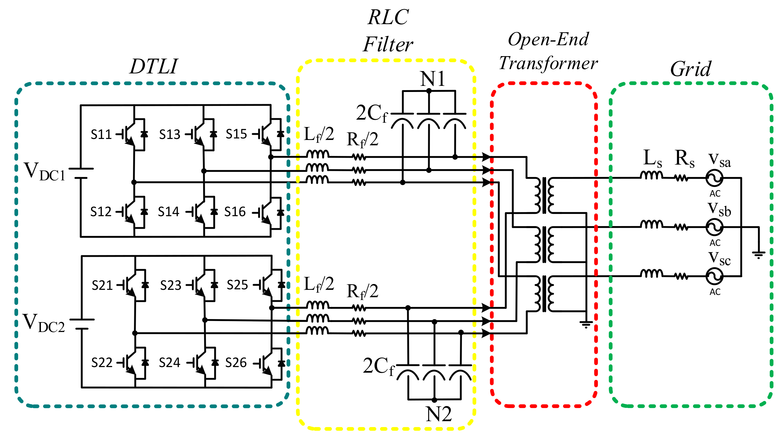
2.1. DTL VSI Configuration

The DTL VSI topology with the common capacitor type (CCT) filter is illustrated in Figure 1. Another conventional DTL VSI arrangement with the individual capacitor type (ICT) filter is depicted in Figure 2. The most important disadvantage of the CCT filter is the inability in fault tolerance. In the ICT filter, when a fault occurs on the DC voltage sources side, another DC voltage source can supply a number of AC loads through its dedicated inverter. Nevertheless, in the CCT filter configuration, the capacitor filters cannot be decoupled from the other side. Therefore, the fault tolerance feature could not be achieved by this type of filter. Compared to the DTL VSI with the ICT filter, the grid current THD, and the cost will be lower in the DTL VSI with the CCT filter. In this paper, since the grid current THD is also studied, the DTL VSI with the CCT filter is implemented.
It is necessary to use an open-end winding transformer in the DTL VSI configuration, which is easily reachable by changing the multi-parallel inverter configuration. Since in the DTL VSI configuration, two TL VSIs are implemented, the voltage level is the same as a three-level NPC inverter from the load point of view. Additionally, the number of switches would be twice that of a TL VSI. Therefore, lower voltage harmonics, decreased rate of change of voltage, alleviated power loss, and also reduced switching frequency are the most important benefits of the DTL VSI, compared with the TL VSI. Consequently, lower harmonics results in a lower rate of device breakdown and a decrease in the size of required filters. Hence, the total expenditures of the power system would be reduced. By employing two DC voltage sources, which are separated, the cancelation of zero sequence current (ZSC) can be achieved. This configuration of DC voltage sources could be simply implemented in photovoltaic systems. In Figure 3, the equivalent circuit of the grid-connected DTL VSI topology with the CCT filter is depicted. According to Figure 3, the state space equations in Section 3 are derived.

2.2. VSG Method

The VSG method, which is used in this paper, is based on the topology that is employed in the VSYNC project. Due to the inherent features of the SGs, the output power of the SG changes during the contingencies’ like load transitions. For example, when a massive increase in the demanded power occurs, the SG slows down and generates extra power in a short time using its stored kinetic energy in its rotating mass. Hence, the frequency drop will be lower. This behavior is according to the swing equation.
P VSG = K DV Δ ω + K IV d Δ ω dt
where PVSG is the output power of the VSG. KDV and KIV are the frequency deviation coefficient and the derivative of the frequency deviation coefficient, respectively. According to equation (1), the extra power, i.e., PVSG, is controllable by two coefficients KDV and KIV. By applying a frequency detection device, i.e., phase-locked loop (PLL), the frequency deviation could be calculated. The coefficient KDV assists in the decrement of frequency deviations during the perturbations, and the coefficient KIV affects the recovery of the rate of change of frequency (ROCOF). It is worth noting that during the disturbances, the larger values of KDV, the more virtual inertia provided by the inverter. Nevertheless, the main problem of large values of KDV is that it can result in oscillated output power of DG and hence, oscillation in system frequency, which may take a few seconds to be completely damped.

3. State-Space Modeling of the System

In this Section, in order to obtain the small-signal analysis of the TL VSI and the DTL VSI, state-space equations of both topologies are written, and all parts of the system, including the current controller, equivalent circuit, PLL, and VSG are considered. Since these equations are nonlinear, the linearization around an operating point is derived in Section 4, and the system’s eigenvalues are evaluated. The model dynamics are considered in the d-q frame.

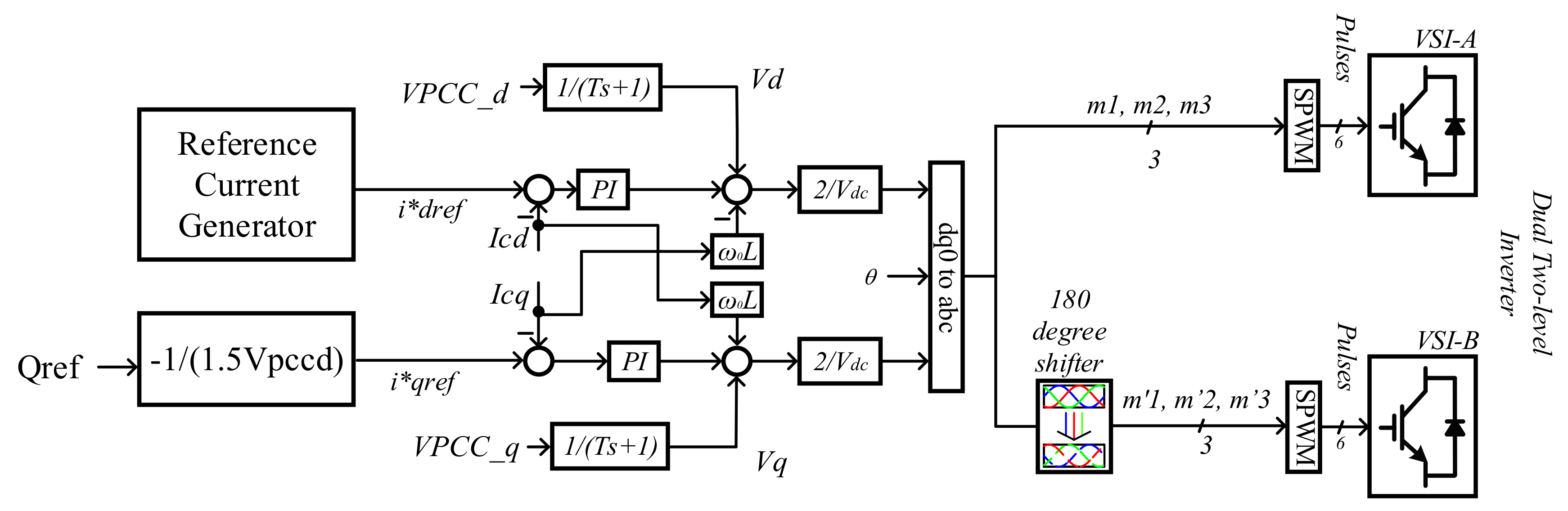
3.1. Current Controller Model

The current controller of the DTL VSI block diagram is shown in Figure 4. The reference current generator block is thoroughly investigated in Section 3.4. By means of the proposed controller, both inverters, which are dedicated to two DC voltage sources of the DTL VSI topology, could be adequately controlled. The DTL VSI controller is the same as the conventional current controller of the TL VSI. The only difference is in the 180-degree phase shifter block, which is shown in Figure 4. The conditions in (2) must be satisfied to obtain the maximum output voltage:
m i = m i                                         i = 1 , 2 , 3 m i = m i + 180 °           i = 1 , 2 , 3
where mi is a reference voltage space vector. The reference current in d frame, i.e., i*dref, which is generated through the reference current generator block, is compared with the inverter’s output current, i.e., icd, and passes through the PI controller to obtain zero steady-state error. Because of using two PI controllers in the d and q frame, two state-space equations are obtained:
d α d dt = i dref * - i cd
d α q dt = i qref - i cq
where α d and α q are the states associated with two PI controllers in d and q frame, respectively. Furthermore, i * qref and i cq are the q frame reference current and the output current of the inverter, respectively. The feed-forward filter is used in this current controller to eliminate the initial transient effect. Due to the appliance of a low pass filter for this aim, two state-space equations in d and q frames are defined as:
dV d dt = V pccd T - V d T
dV q dt = V pccq T - V q T
where Vpccd and Vpccq are the voltages measured at the point of common coupling (PCC) and are passed through the feed-forward filter to obtain the output voltages, which are Vd and Vq.
Vcd and Vcq are the command signals of the output voltages of the inverters. According to Figure 4, the command signals are defined as two equations below where Kp, ω(t), Ki, Lf, and Rf are proportional gain of PI controller, angular frequency of the system which is realized by the PLL, the integral gain of PI controller, and the LC filter’s inductance and its resistance, respectively.
V cd = K pi i dref * - K pi i cd + K ii α d - L f ω t i cq + V d + R f i cd
V cq = K pi i qref - K pi i cq + K ii α q + L f ω t i cd + V q + R f i cq

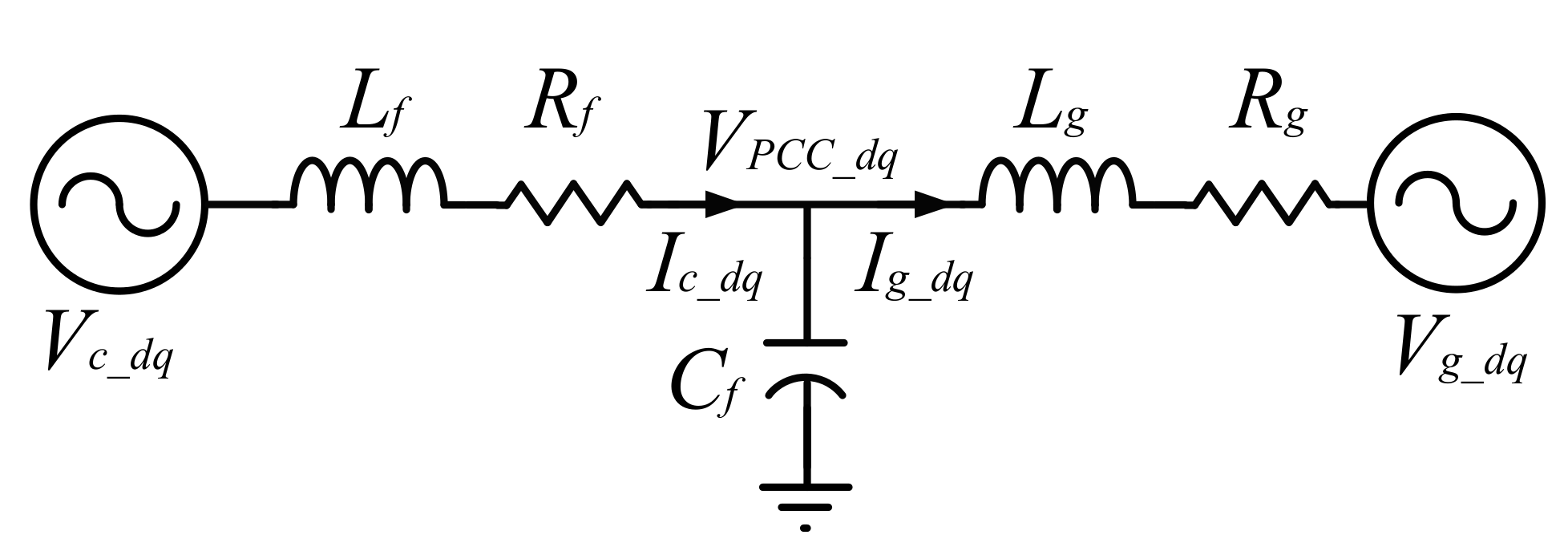
3.2. Equations of the Equivalent Circuit of the TL VSI

The equivalent circuit of the TL VSI is depicted in Figure 5. By neglecting the switches’ losses, the Vcd and Vcq, described in the latter Section, could be considered as the output voltage of the inverter. Therefore, the following equations are derived.
L f di cd dt = - V pccd + V cd - R f i cd + L f ω t i cq
L f di cq dt = - V pccq + V cq - R f i cq - L f ω t i cd
L g di gd dt = V pccd - V gd - R g i gd + L g ω t i gq
L g di gq dt = V pccq - V gq - R g i gq - L g ω t i gd
C f dV pccd dt = i cd - i gd + C f ω t V pccq
C f dV pccq dt = i cq - i gq - C f ω t V pccd
where igdq, Vgdq, Lg, Rg, and Cf are the grid current and the grid voltage in the d-q frame, the grid inductance, the grid resistance, and the filter capacitor, respectively. By substituting (7) and (8) in (10) and (11), the equations are rewritten as:
L f di cd dt = - V pccd + K ii α d + K pi i dref * - K p i cd + V d .
L f di cq dt = - V pccq + K ii α q + K pi i qref - K p i cq + V q

3.3. Equations of the Equivalent Circuit of the DTL VSI

The equivalent circuit of the DTL VSI is illustrated in Figure 3. Equations (11) (14) are the same for the DTL VSI topology. Another two different equations are established as below:
L f di cd dt = - V pccd + 2 V cd - R f i cd + L f ω t i cq
L f di cq dt = - V pccq + 2 V cq - R f i cq - L f ω t i cd
By replacing (7) and (8) in (17) and (18), these two state-space equations are realized as:
L f di cd dt = - V pccd + 2 K ii α d + 2 K pi i dref * - 2 K pi i cd + 2 V d - L f ω t i cq + R f i cd - V pccd
L f di cq dt = - V pccq + 2 K ii α q + 2 K pi i qref - 2 K pi i cq + 2 V q + L f ω t i cd + R f i cq - V pccq

3.4. Phase-Locked Loop
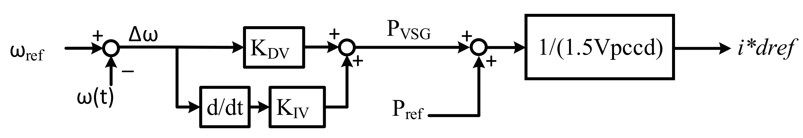
The conventional block diagram of the PLL is depicted in Figure 6. The main task of the PLL is to make sure that φ equals ω 0 t + θ 0 . Therefore, Vpccq will be zero in steady-state. To do so, a controller, i.e., H(s), must contain at least one integrator to be developed in the control loop to obtain zero steady-state error, as mentioned in [30]. In this paper, a Proportional Integral Derivative (PID) controller is applied. Therefore, the transfer function of the H(s) is as (21).
H s = K I + K P s + K D s 2 s
where KP, KI, and KD are the proportional, integral, and derivative coefficients of the PID controller, respectively. Therefore, as mentioned in [30], by implementing the diagonal canonical form of the PID controller, two state-space equations are defined as follows.
d α 1 PID dt = - C 1 α 1 PID + V pccq
d α 2 PID dt = - C 2 α 2 PID + V pccq
where α 1 PID and α 2 PID are two states related to the PID controllers in the d-q frame. Furthermore, C1 and C2 are constants, which cause the numerator and denominator degree of the H(s) to become identical in order to have a proper transfer function. Additionally, the value of C1 and C2 is mentioned in the Appendix (Table A1). The state-space model of the system with an integrator shown in Figure 6 can be written as follows.
d φ dt = ω t = m 1 α 1 PID + m 2 α 2 PID + K D C 2 V pccq
where m1 and m2 are obtained from the equations below [30].
m 1 = K I + K P s + K D s 2 C 2 s + 1             s = - C 1 m 2 = 1 C 2 K I + K P s + K D s 2 s + C 1             s = - 1 / C 2

3.5. VSG Controller

In this Section, the reference current generator block in Figure 4 is described. The detailed block diagram of the reference current generator block is illustrated in Figure 7. As can be seen, the inverter’s reference current command signal, i.e., i*dref, is composed of iVSG and idref.
i dref * = P VSG + P ref 1 . 5 V pccd = i dref + K DV 2 π f 0 - ω t + K IV ( d 2 π f 0 - ω t dt ) 1.5 V pccd = i dref - K DV * ω t - K IV * d ω t dt + 2 π f 0 K DV *
By substituting (22) (24) and (14) in (26), i*dref could be rewritten as (27).
i dref * = i dref + 2 π f 0 K DV * + α 1 PID - m 1 K DV * + m 1 C 1 K IV * + m 1 K D K IV * C 2 V pccd + α 2 PID - m 2 K DV * + m 2 C 2 K IV * + m 2 K D K IV * C 2 V pccd + V pccq - m 1 K DV * - m 2 K IV * + K D 2 K IV * C 2 2 V pccd - K DV * K D C 2 - i cq K D K IV * C 2 C f + i gq K D K IV * C 2 C f

4. Small-Signal Modelling and Simulation Verifications

In this Section, according to (28) and (29), in order to realize the whole eigenvalues and analyze them, the state-spaces of the TL VSI and the DTL VSI are linearized around the operating points, which are denoted by subscript 0. By increasing the coefficient KDV, the eigenvalues migration of the TL VSI and the DTL VSI are compared to each other, and the stability enhancement in the DTL VSI is investigated. Additionally, the ability of the DTL VSI in damping the oscillations is evaluated.
Δ DTL   VSI = A DTL   VSI Δ x DTL   VSI + B DTL   VSI Δ u
Δ TL   VSI = A TL   VSI Δ x TL   VSI + B TL   VSI Δ u
where x DTL   VSI and x TL   VSI , representing vectors of the state variables, are the same and could be described as (30). All of the matrices in (28) and (29) are entirely given in the Appendix.
Δ x DTL   VSI ,   TL   VSI = Δ i cd   Δ i cq   Δ α d   Δ α q   Δ V pccd   Δ V pccq   Δ i gd   Δ i gq   Δ V d   Δ V q   Δ α 1 PID   Δ α 2 PID   Δ φ T

4.1. Dominant Eigenvalues Analysis of the TL VSI and the DTL VSI

In this Section, in order to compare the effect of the virtual inertia on the stability of the TL VSI and the DTL VSI, the dominant eigenvalues of the TL VSI and the DTL VSI are demonstrated in Figure 8. It is assumed that the values of the coefficient KDV and the coefficient KIV in the swing equation are the same for both topologies. The eigenvalues of the TL VSI are shown by blue multiplication signs, and the eigenvalues of the DTL VSI are illustrated by red plus signs. As it is depicted in Figure 8b,c, two eigenvalues of the DTL VSI are the same as the TL VSI. Another two eigenvalues of the DTL VSI are farther from the jω-axis compared with the TL VSI eigenvalues. Therefore, compared with the TL VSI, the system’s stability is enhanced in the DTL VSI.

4.2. Oscillation Damping Ability of the DTL VSI and the TL VSI

As mentioned in the latter Section, larger values of the virtual inertia coefficient, i.e., KDV, could lead to fluctuations in the system, which may take a few seconds to be thoroughly damped. In order to illustrate these fluctuations, the simulation results are obtained in the next Section. All eigenvalues of the grid-connected TL VSI and the grid-connected DTL VSI are shown in Figure 9 and Figure 10, respectively. In both figures, the migration of the eigenvalues is started with a green sign and ended with a red sign, and the coefficient KDV is increased from 0 to 5000. The eigenvalues of the TL VSI are depicted by multiplication signs, and the eigenvalues of the DTL VSI are shown by plus signs.
As expected, in Figure 9, two eigenvalues move on the real axis, and by increasing the coefficient KDV, they take distance from the real axis and become a complex number. By increasing the coefficient KDV, only these two eigenvalues move away from the real axis. Therefore, the oscillations, which happen in the system by large values of the coefficient KDV, are only because of these two eigenvalues in the grid-connected TL VSI. It is noteworthy that these two eigenvalues are not dominant, but regarding the amount of their imaginary term, they can have an influence on the operation of the whole system. In Figure 10, as it is depicted, the DTL VSI eigenvalues migrate on the real axis, and by increasing the coefficient KDV, they remain a real number. Thus, it can be deduced that by higher values of the virtual inertia coefficient, the fluctuations are eliminated in the grid-connected DTL VSI. It must be noted that the dominant eigenvalues, which are illustrated in Figure 8, are not shown in Figure 9 and Figure 10 for more clarity.

4.3. Simulation Results

In this Section, in order to confirm the small-signal analysis presented in the previous Section, the simulation results are presented. Note that all parameters of the small-signal analysis and the simulations are given in the Appendix (Table A1). All of the parameters of the grid-connected TL VSI and grid-connected DTL VSI are the same, and the virtual inertia coefficient, i.e., KDV in both systems, is 3000. As it is depicted in Figure 11, by a change in the demanded active power of the load, the grid-connected TL VSI frequency oscillates, but the grid-connected DTL VSI frequency eliminates these oscillations.

5. Grid Current THD Reduction in the DTL VSI Topology

As explained before, one of the most important benefits of the DTL VSI is lower voltage and current harmonics. In this Section, in order to study the abilities of the TL VSI and the DTL VSI to supply a nonlinear load, the controller that is presented in the reference [29] is introduced, and the grid current THD of the TL VSI and the DTL VSI is compared in the simulations part.
The difference between the conventional controller and the controller proposed in reference [29] is in the reference current generator block. By means of the reference current generator block, which is proposed in reference [29], the DG could be able to compensate harmonic load current components while it is integrated into the utility grid. In Figure 12, the reference current generator is illustrated. As can be seen, by means of a low pass filter, the harmonic component of the load current is added to the reference current, i.e., iref in the d frame. Therefore, the grid current’s harmonic components could be lower, and the DG compensates these components.

Simulation Results and the Grid Current Analysis

Similar to the reference [29], in order to simulate a nonlinear load, diodes are applied at the load point where a resistive-inductive load exists. The simulation results of the TL VSI and the DTL VSI are demonstrated in Figure 13 and Figure 14, respectively. In both figures, the utility grid supplies nonlinear load until t = 0.1 s. At this moment, the DG is connected to the grid, and due to the controller method introduced in the prior Section, the DG supplies the nonlinear load. Therefore, the grid current will be equal to zero. At t = 0.2 s, another similar nonlinear load is connected to the load point.
Since the maximum active and reactive power of the DG is less than the demanded active and reactive power of loads, the DG provides its maximum active and reactive power and supplies harmonic components of loads, and the remaining active and reactive requested power of loads is generated by the utility grid. This process is carried on until t = 0.35 s. In this period, as it is depicted in Figure 13 and Figure 14, compared with the grid-connected TL VSI, the grid current THD is reduced in the grid-connected DTL VSI simulation. Using the MATLAB software’s FFT analysis tool, the grid current THD of the grid-connected TL VSI and the grid-connected DTL VSI is 7.83% and 0.97%, respectively. Therefore, the grid current THD reduction in the DTL VSI could be concluded. At t = 0.35 s, the added nonlinear load is disconnected from the demand side, and the grid current becomes zero again.

6. Performance Comparison Between the TL VSI and the DTL VSI

In order to benefit the advantages of the DTL VSI, which is investigated in the prior Sections, a proper reference current command signal is designed. The proposed reference current generator block diagram is shown in Figure 15. Through the illustrated block diagram, stability enhancement, oscillation damping during the contingencies, and the ability to alleviate the grid current THD could be investigated in both topologies, i.e., the TL VSI and the DTL VSI, simultaneously.

6.1. Simulation Results of the Proposed Controller

In this Section, in order to demonstrate decreased frequency deviations adequately and evaluate the VSG controller operation, a 20kVA synchronous generator is utilized instead of a utility grid. In two cases, the simulation results are derived. In both cases, the virtual inertia coefficient, i.e., KDV, is 4000.

6.1.1. Case A: Grid-Connected TL VSI

In this case, the proposed reference current generator block is applied to control the grid-connected TL VSI. Until t = 0.5 s, the SG supplies the nonlinear load. At this moment, the DG is connected to SG, and as discussed in Section 5, the SG current will be equal to zero. This process continues until t = 1.6 s. At t = 1.6 s, another similar load is connected. At this moment, since the frequency deviates from its nominal value, the VSG controller attempts to provide extra power to prevent large frequency variations. Due to the analysis presented in Section 4, owing to the fact that the inertia coefficient is large, fluctuations happen in the system frequency and the output power of the DG. In Figure 16 and Figure 17, the load, SG, and DG current are depicted. As it is demonstrated in Figure 17 when the nonlinear load is connected, the VSG induces oscillations in the system, and therefore, after t = 1.6 s, the SG current is not sinusoidal, and the DG operation is not proper. The system frequency in two situations without inertia and with inertia is illustrated in Figure 18. The output active power of the DG is shown in Figure 19. Fluctuations are observed in Figure 18 and Figure 19. As mentioned before, these fluctuations could take a few seconds to be completely damped.

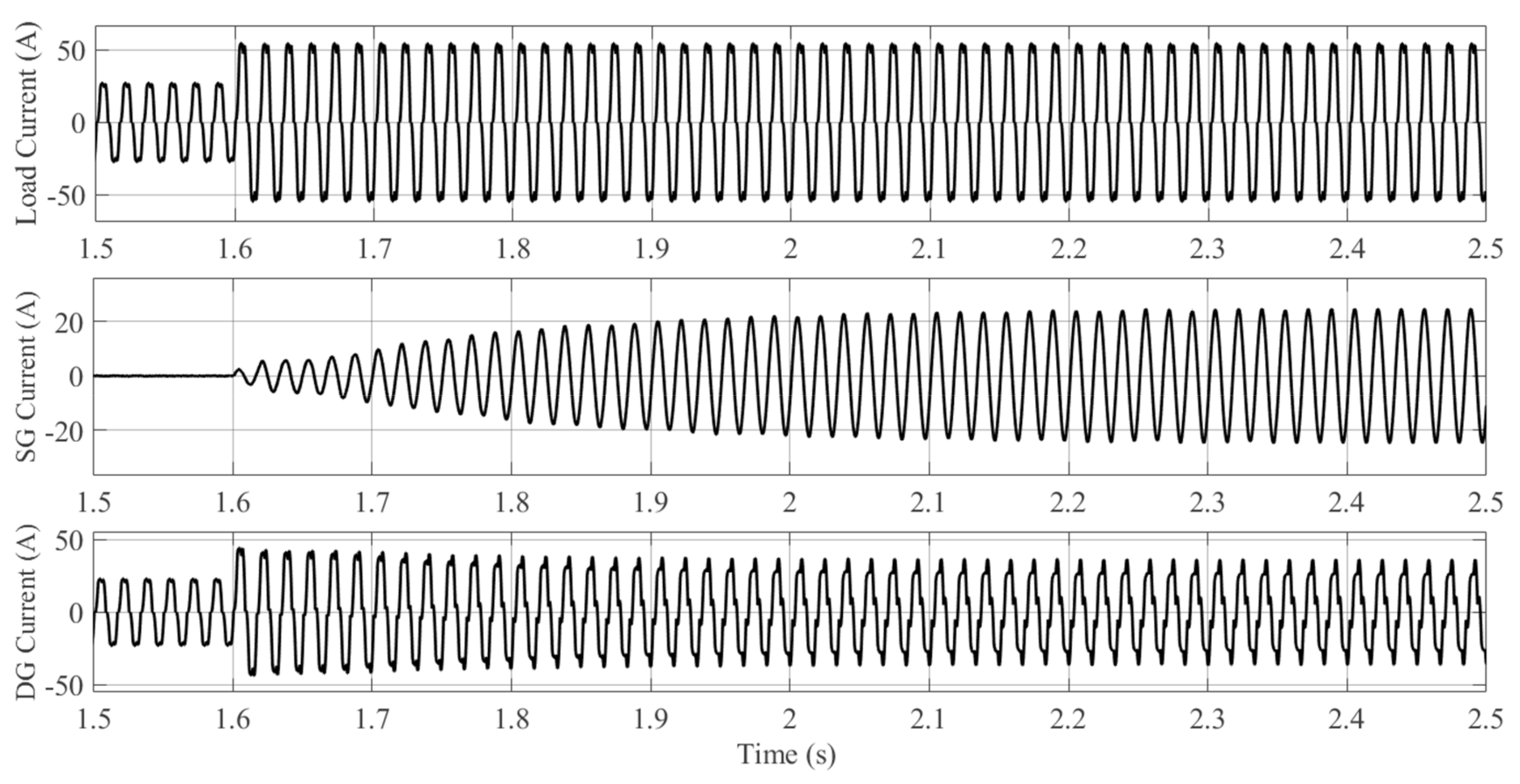
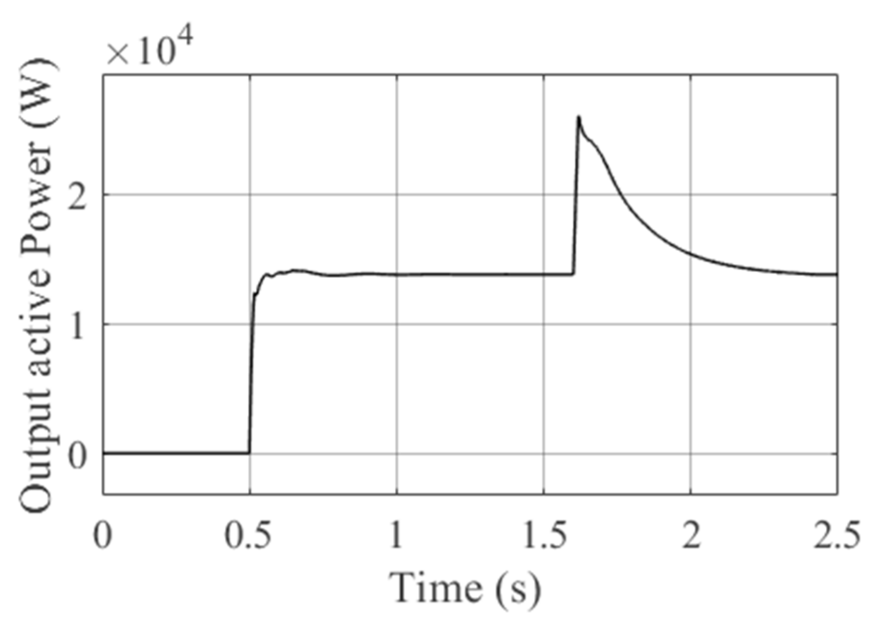
6.1.2. Case B: Grid-Connected DTL VSI

The process arranged in this case is the same as Case A. The DG is connected to the SG at t = 0.5 s, as it is shown in Figure 20. After the connection of another nonlinear load, which is similar to the prior nonlinear load, as it is demonstrated in Figure 21, it can be seen that unlike the simulations of the grid-connected TL VSI, the grid-connected DTL VSI can damp the system oscillations completely, and the SG current will be in a sinusoidal form. Therefore, as investigated in Section 4, in the presence of the VSG controller, the grid-connected DTL VSI operates appropriately. After t = 1.6 s, the DG compensates the load current’s harmonic components and injects its maximum active and reactive power. The remaining demanded power is supplied by the SG. The transient response in the SG current, which is demonstrated in Figure 21, is because of the VSG controller, and from the utility grid (or SG in this case) point of view, the inverter looks like a synchronous generator.
In Figure 22, the system frequency with and without virtual inertia is depicted. As can be seen, the frequency deviation during the contingency is alleviated compared to the system without virtual inertia. The output active power of the DTL VSI is illustrated in Figure 23. In this case, no fluctuations are observed, and the simulation results prove the analysis of the eigenvalues derived in Section 4.

7. Conclusions

Due to DG’s increasing penetration rate, the VSG controller is one of the most important parts of the upcoming controller design. In this paper, the grid-connected DTL VSI advantages in improving the power system stability and damping the system fluctuations while utilizing the VSG controller were proven through the small-signal analysis and simulation results. The state-space equations of the grid-connected DTL VSI and the grid-connected TL VSI, considering the presence of the PLL and the VSG controller, were obtained. The small-signal analysis showed how poles are moved by increasing the inertia coefficient and which poles will be the cause of fluctuations in the system. Moreover, the small-signal analysis of the DTL VSI was derived, and it was proven that larger values of the virtual inertia coefficient in conventional topology, i.e., TL VSI, could result in fluctuations in the power system. However, by using the DTL VSI, the fluctuations could be eliminated. Furthermore, in the DTL VSI configuration, the power system is more stable than the TL VSI configuration. Furthermore, the DTL VSI benefits in reducing grid current THD were demonstrated. A reference current command signal was designed to simultaneously supply nonlinear loads and emulate the transient behavior of SGs during the contingencies. The simulation results proved that compared to the grid-connected TL VSI, the grid-connected DTL VSI enhanced the performance and the stability of the system and dampened the oscillations that occur in the conventional grid-connected TL VSI.

Author Contributions

Conceptualization, M.A.D., H.N. and E.P.; Methodology, M.A.D.; Validation, H.N., E.P. and A.K.; Formal analysis, M.A.D.; Investigation, M.A.D.; Writing—original draft preparation, M.A.D.; Writing—review and editing, H.N., E.P., A.K. and M.H.; Supervision, H.N., E.P., A.K. and M.H. All authors have read and agreed to the published version of the manuscript.

Funding

This research received no external funding.

Institutional Review Board Statement

Not applicable.

Informed Consent Statement

Not applicable.

Data Availability Statement

The data presented in this study are available on request from the corresponding author.

Conflicts of Interest

The authors declare no conflict of interest.

Appendix A

Table A1. System parameters.
ParameterValue
PID controller of the PLL coefficients (KP/KI/KD)180/3200/1
DC link voltage (VDC)500 V
RLC filter resistance, inductance and capacitance (Rf/Lf/Cf)0.01 Ω/0.0024 H/10−6 F
Line to line rms voltage (VLLrms) 25,000 V
Nominal frequency (f0)60 HZ
C1/C20.001/0.001
Switching frequency8000 HZ
Transformer ratio1:96.15
Nonlinear loads inductance and resistance0.01 H/20 Ω
PI Current controller (Kpi/Kii)1000/30
The low-pass filter time constant (T)0.05
The grid inductance and resistance (Lg/Rg) 2083.3 377 2 H/ 2083.3 2   Ω
SCCR10
Nominal rated power of the inverter30 kVA
A DTL   VSI = M - 1 A 11 DTL A 12 DTL A 21 DTL A 22 DTL
A TL   VSI = N - 1 A 11 TL A 12 TL A 21 TL A 22 TL
where matrixes M , A 21 DTL , A 22 DTL , and A 21 TL , A 22 TL , N are the same, respectively.
A 11 DTL = R 2 K pi a 1 , 2 2 K ii 0 a 1 , 5 a 1 , 6 0 L f ω 0 R 2 K pi 0 2 K ii 0 i cd 0 L f K D C 2 1 0 1 K IV * K D C 2 C f 0 0 1 + a 1 , 5 2 K pi ( i cq 0 L f K D C 2 + a 1 , 6 ) 2 K pi 0 0 1 0 0 0 0 0 1 0 0 0 0 C f ( m 1 α 1 PID 0 + m 2 α 2 PID 0 + 2 K D C 2 V pccq 0 ) 1 0 1 0 0 C f ω 0 C f K D C 2 V pccq 0 0 0 0 0 0 1 L g K D C 2 i gq 0 R g
A 12 DTL = 2 K IV * K D K pi C 2 C f 2 0 a 1 , 11 a 1 , 12 0 0 0 2 i cd 0 L f m 1 i cq 0 L f m 2 K IV * K D C 2 C f 0 0 ( i cd 0 L f m 1 + a 1 , 11 ) 2 K pi ( i cq 0 L f m 2 + a 1 , 12 ) 2 K pi 0 0 0 0 0 0 0 0 0 C f m 1 V pccq 0 C f m 2 V pccq 0 0 1 0 0 C f m 1 V pccd 0 C f m 2 V pccd 0 0 L g ω 0 0 0 L g m 1 i gq 0 L g m 2 i gq 0 2 3 V llrms sin α 0
A 21 DTL = 0 0 0 0 0 1 L g K D C 2 i gd 0 L g ω 0 0 0 0 0 1 T 0 0 0 0 0 0 0 1 T 0 0 0 0 0 0 1 0 0 0 0 0 0 1 0 0 0 0 0 0 K D C 2 0
A 22 DTL = L g 0 0 L g m 1 i dg 0 L g m 1 i gq 0 2 3 V llrms sin α 0 0 1 T 0 0 0 0 0 0 1 T 0 0 0 0 0 0 C 1 0 0 0 0 0 0 C 2 0 0 0 0 m 1 m 2 0
A 11 TL = K pi K IV * K D C 2 C f K pi K ii 0 ( a 1 , 5 1 ) 2 ( a 1 , 6 + i cq 0 L f K D C 2 ) 2 0 0 K pi 0 K ii 0 1 0 1 K IV * K D C 2 C f 0 0 ( 1 + a 1 , 5 ) 2 K pi ( i cq 0 L f K D C 2 + a 1 , 6 ) 2 K pi 0 0 1 0 0 0 0 0 1 0 0 0 0 C f ( m 1 α 1 PID 0 + m 2 α 2 PID 0 + 2 K D C 2 V pccq 0 ) 1 0 1 0 0 C f ω 0 C f K D C 2 V pccq 0 0 0 0 0 0 1 L g K D C 2 i gq 0 R g
A 12 TL = K IV * K D K pi C 2 C f 1 0 ( a 1 , 11 + i cq 0 L f m 1 ) 2 ( a 1 , 12 + i cq 0 L f m 2 ) 2 0 0 0 1 0 0 0 K IV * K D C 2 C f 0 0 ( i cq 0 L f m 1 + a 1 , 11 ) 2 K pi ( i cq 0 L f m 2 + a 1 , 12 ) 2 K pi 0 0 0 0 0 0 0 0 0 0 C f m 1 V pccq 0 C f m 2 V pccq 0 0 1 0 0 C f m 1 V pccd 0 C f m 2 V pccd 0 0 L g ω 0 0 0 L g m 1 i gq 0 L g m 2 i gq 0 2 3 V llrms sin α 0
M = L f 0 0 0 0 0 0 0 0 0 0 0 0 0 L f 0 0 0 0 0 0 0 0 0 0 0 0 0 1 0 0 0 0 0 0 0 0 0 0 0 0 0 1 0 0 0 0 0 0 0 0 0 0 0 0 0 C f 0 0 0 0 0 0 0 0 0 0 0 0 0 C f 0 0 0 0 0 0 0 0 0 0 0 0 0 L g 0 0 0 0 0 0 0 0 0 0 0 0 0 L g 0 0 0 0 0 0 0 0 0 0 0 0 0 1 0 0 0 0 0 0 0 0 0 0 0 0 0 1 0 0 0 0 0 0 0 0 0 0 0 0 0 1 0 0 0 0 0 0 0 0 0 0 0 0 0 1 0 0 0 0 0 0 0 0 0 0 0 0 0 1
a 1 , 2 = L f ( m 1 α 1 PID 0 + m 2 α 2 PID 0 + K D C 2 V pccq 0 + 2 K IV * K D K pi L f C 2 C f ) a 1 , 5 = 1 + 2 α 1 PID 0 m 1 K D K IV * K pi C 2 + 2 α 2 PID 0 m 2 K D K IV * K pi C 2 + 2 V pccq 0 K D 2 K IV K pi C 2 2 a 1 , 6 = i cq 0 L f 2 K D C 2 + 2 V pccd 0 K D 2 K IV * K pi C 2 2 2 K D K DV * K pi C 2 2 m 1 K IV * K P 2 m 2 K IV * K p a 1 , 11 = i cq 0 L f m 1 2 V pccd 0 m 1 K D K IV * K pi C 2 2 m 1 K DV * K pi + 2 m 1 C 1 K DV * K pi a 1 , 12 = i cq 0 L f m 2 2 V pccd 0 m 2 K D K IV * K pi C 2 2 m 2 K DV * K pi + 2 m 2 C 2 K DV * K pi ω 0 = m 1 α 1 PID 0 + m 2 α 2 PID 0 K D C 2 V pccq 0
B DTL   VSI = 2 π K DV * 2 K pi 0 0 0 2 K pi 2 π K DV * 1 0 0 0 1 0 0 0 0 0 0 0 0 0 0 0 0 0 0 0 0 0 0 0 0 0 0 0 0 0 0 0 f 0 I dref I qref
B TL   VSI = 2 π K DV * K pi 0 0 0 K pi 2 π K DV * 1 0 0 0 1 0 0 0 0 0 0 0 0 0 0 0 0 0 0 0 0 0 0 0 0 0 0 0 0 0 0 0 f 0 I dref I qref

References

  1. Tamrakar, U.; Shrestha, D.; Maharjan, M.; Bhattarai, B.P.; Hansen, T.M.; Tonkoski, R. Virtual Inertia: Current Trends and Future Directions. Appl. Sci. 2017, 7, 654. Available online: https://www.mdpi.com/2076-3417/7/7/654#cite (accessed on 19 February 2021). [CrossRef]
  2. Driesen, J.; Visscher, K. Virtual synchronous generators. In Proceedings of the IEEE Power and Energy Society 2008 General Meeting: Conversion and Delivery of Electrical Energy in the 21st Century, Pittsburgh, PA, USA, 20–24 July 2008. [Google Scholar]
  3. Loix, T.; De Breucker, S.; Vanassche, P.; Van Den Keybus, J.; Driesen, J.; Visscher, K. Layout and performance of the power electronic converter platform for the VSYNC project. In Proceedings of the 2009 IEEE Bucharest PowerTech: Innovative Ideas Toward the Electrical Grid of the Future, Bucharest, Romania, 28 June–2 July 2009. [Google Scholar]
  4. Zhong, Q.C.; Weiss, G. Synchronverters: Inverters that mimic synchronous generators. IEEE Trans. Ind. Electron. 2011. [Google Scholar] [CrossRef]
  5. Zhong, Q.C.; Nguyen, P.L.; Ma, Z.; Sheng, W. Self-synchronized synchronverters: Inverters without a dedicated synchronization unit. IEEE Trans. Power Electron. 2014. [Google Scholar] [CrossRef]
  6. Ashabani, M.; Mohamed, Y.A.R.I. Integrating VSCs to weak grids by nonlinear power damping controller with self-synchronization capability. IEEE Trans. Power Syst. 2014. [Google Scholar] [CrossRef]
  7. Huang, L.; Xin, H.; Wang, Z.; Wu, K.; Wang, H.; Hu, J.; Lu, C. A Virtual Synchronous Control for Voltage-Source Converters Utilizing Dynamics of DC-Link Capacitor to Realize Self-Synchronization. IEEE J. Emerg. Sel. Top. Power Electron. 2017. [Google Scholar] [CrossRef]
  8. Mishra, S.; Pullaguram, D.; Buragappu, S.A.; Ramasubramanian, D. Single-phase synchronverter for a gridconnected roof top photovoltaic system. IET Renew. Power Gener. 2016. [Google Scholar] [CrossRef]
  9. Yap, K.Y.; Sarimuthu, C.R.; Lim, J.M.Y. Grid Integration of Solar Photovoltaic System Using Machine Learning-Based Virtual Inertia Synthetization in Synchronverter. IEEE Access. 2020. [Google Scholar] [CrossRef]
  10. Shuai, Z.; Huang, W.; Shen, Z.J.; Luo, A.; Tian, Z. Active Power Oscillation and Suppression Techniques between Two Parallel Synchronverters during Load Fluctuations. IEEE Trans. Power Electron. 2020. [Google Scholar] [CrossRef]
  11. Rosso, R.; Engelken, S.; Liserre, M. Robust stability analysis of synchronverters operating in parallel. IEEE Trans. Power Electron. 2019. [Google Scholar] [CrossRef]
  12. Sakimoto, K.; Miura, Y.; Ise, T. Stabilization of a power system with a distributed generator by a Virtual Synchronous Generator function. In Proceedings of the 8th International Conference on Power Electronics—ECCE Asia, Jeju, Korea, 29 May–2 June 2011; pp. 1498–1505. Available online: https://ieeexplore.ieee.org/document/5944492 (accessed on 19 February 2021).
  13. Soni, N.; Doolla, S.; Chandorkar, M.C. Improvement of transient response in microgrids using virtual inertia. IEEE Trans. Power Deliv. 2013. [Google Scholar] [CrossRef]
  14. Liu, J.; Miura, Y.; Ise, T. Comparison of Dynamic Characteristics Between Virtual Synchronous Generator and Droop Control in Inverter-Based Distributed Generators. IEEE Trans. Power Electron. 2016, 31, 3600–3611. Available online: https://ieeexplore.ieee.org/document/7182342 (accessed on 19 February 2021). [CrossRef]
  15. Torres, L.M.A.A.; Lopes, L.A.C.; Morán, T.L.A.A.; Espinoza, C.J.R. Self-tuning virtual synchronous machine: A control strategy for energy storage systems to support dynamic frequency control. IEEE Trans. Energy Convers. 2014. [Google Scholar] [CrossRef]
  16. Alipoor, J.; Miura, Y.; Ise, T. Power system stabilization using virtual synchronous generator with alternating moment of inertia. IEEE J. Emerg. Sel. Top. Power Electron. 2015. [Google Scholar] [CrossRef]
  17. Li, D.; Zhu, Q.; Lin, S.; Bian, X.Y. A Self-Adaptive Inertia and Damping Combination Control of VSG to Support Frequency Stability. IEEE Trans. Energy Convers. 2017. [Google Scholar] [CrossRef]
  18. Fang, J.; Li, H.; Tang, Y.; Blaabjerg, F. Distributed Power System Virtual Inertia Implemented by Grid-Connected Power Converters. IEEE Trans. Power Electron. 2018. [Google Scholar] [CrossRef] [Green Version]
  19. Fang, J.; Lin, P.; Li, H.; Yang, Y.; Tang, Y. An improved virtual inertia control for three-phase voltage source converters connected to a weak grid. IEEE Trans. Power Electron. 2019. [Google Scholar] [CrossRef] [Green Version]
  20. Saeedian, M.; Eskandari, B.; Taheri, S.; Hinkkanen, M.; Pouresmaeil, E. A Control Technique Based on Distributed Virtual Inertia for High Penetration of Renewable Energies Under Weak Grid Conditions. IEEE Syst. J. 2020. [Google Scholar] [CrossRef]
  21. Ashabani, M.; Freijedo, F.D.; Golestan, S.; Guerrero, J.M. Inducverters: PLL-Less Converters With Auto-Synchronization and Emulated Inertia Capability. IEEE Trans. Smart Grid 2016. [Google Scholar] [CrossRef]
  22. Yan, X.; Mohamed, S.Y.A.; Li, D.; Gadalla, A.S. Parallel operation of virtual synchronous generators and synchronous generators in a microgrid. J. Eng. 2019. [Google Scholar] [CrossRef]
  23. Zhao, H.; Yang, Q.; Zeng, H. Multi-loop virtual synchronous generator control of inverter-based DGs under microgrid dynamics. IET Gener. Transm. Distrib. 2017. [Google Scholar] [CrossRef]
  24. Dashtaki, M.A.; Nafisi, H.; Pouresmaeil, E.; Khorsandi, A. Virtual Inertia Implementation in Dual Two-Level Voltage Source Inverters. In Proceedings of the 2020 11th Power Electronics, Drive Systems, and Technologies Conference (PEDSTC), Tehran, Iran, 4–6 February 2020; pp. 1–6. Available online: https://ieeexplore.ieee.org/document/9088389 (accessed on 19 February 2021). [CrossRef]
  25. Aghazadeh, A.; Jafari, M.; Khodabakhshi-Javinani, N.; Nafisi, H.; Jabbari Namvar, H. Introduction and advantage of space opposite vectors modulation utilized in dual two-level inverters with isolated DC sources. IEEE Trans. Ind. Electron. 2019. [Google Scholar] [CrossRef]
  26. Manoj Kumar, M.V.; Mishra, M.K.; Kumar, C. A Grid-Connected Dual Voltage Source Inverter with Power Quality Improvement Features. IEEE Trans. Sustain. Energy 2015. [Google Scholar] [CrossRef]
  27. Wang, B.; Zhang, X.; Song, C.; Cao, R. Research on the filters for dual-inverter fed open-end winding transformer topology in photovoltaic grid-tied applications. Energies 2019, 2338. [Google Scholar] [CrossRef] [Green Version]
  28. Gohil, G.; Bede, L.; Teodorescu, R.; Kerekes, T.; Blaabjerg, F. Dual-Converter-Fed Open-End Transformer Topology with Parallel Converters and Integrated Magnetics. IEEE Trans. Ind. Electron. 2016. [Google Scholar] [CrossRef] [Green Version]
  29. Pouresmaeil, E.; Miguel-Espinar, C.; Massot-Campos, M.; Montesinos-Miracle, D.; Gomis-Bellmunt, O. A control technique for integration of DG units to the electrical networks. IEEE Trans. Ind. Electron. 2013. [Google Scholar] [CrossRef]
  30. Aghazadeh, A.; Davari, M.; Nafisi, H.; Blaabjerg, F. Grid Integration of a Dual Two-Level Voltage-Source Inverter considering Grid Impedance and Phase-Locked Loop. IEEE J. Emerg. Sel. Top. Power Electron. 2019. [Google Scholar] [CrossRef]
Figure 1. Dual two-level voltage source inverter (DTL VSI) topology with the common capacitor type (CCT) filter.
Energies 14 01160 g001
Figure 2. DTL VSI topology with the individual capacitor type (ICT) filter.
Energies 14 01160 g002
Figure 3. DTL VSI equivalent circuit.
Energies 14 01160 g003
Figure 4. The current controller block diagram.
Energies 14 01160 g004
Figure 5. Two-level voltage source inverter (TL VSI) equivalent circuit.
Energies 14 01160 g005
Figure 6. Phase-locked loop (PLL) block diagram.
Energies 14 01160 g006
Figure 7. The detailed reference current generator block.
Energies 14 01160 g007
Figure 8. (a) Dominant Eigenvalues of the TL VSI and the DTL VSI; (b,c) zoomed photos of (a).
Energies 14 01160 g008
Figure 9. The TL VSI eigenvalues.
Energies 14 01160 g009
Figure 10. The DTL VSI eigenvalues.
Energies 14 01160 g010
Figure 11. System frequency of the grid-connected TL VSI and grid-connected DTL VSI.
Energies 14 01160 g011
Figure 12. Reference current generator block diagram in [29].
Energies 14 01160 g012
Figure 13. TL VSI simulation results.
Energies 14 01160 g013
Figure 14. DTL VSI simulation results.
Energies 14 01160 g014
Figure 15. The proposed reference current generator block diagram.
Energies 14 01160 g015
Figure 16. Load, synchronous generators (SG), and distributed generations (DG) currents before and after connecting the DG.
Energies 14 01160 g016
Figure 17. Load, SG, and DG currents before and after connecting the additional nonlinear load.
Energies 14 01160 g017
Figure 18. System frequency with and without virtual inertia.
Energies 14 01160 g018
Figure 19. Output active power of the DG.
Energies 14 01160 g019
Figure 20. Load, SG and DG currents before and after connection of the DG to the SG at t = 0.5 s.
Energies 14 01160 g020
Figure 21. Load, SG and DG currents before and after connection of the additional nonlinear load at t = 1.6 s.
Energies 14 01160 g021
Figure 22. System frequency with and without virtual inertia.
Energies 14 01160 g022
Figure 23. Output active power of the DG.
Energies 14 01160 g023
Publisher’s Note: MDPI stays neutral with regard to jurisdictional claims in published maps and institutional affiliations.

