Power Forecasting of a Photovoltaic Plant Located in ENEA Casaccia Research Center

Abstract

This work proposes an Artificial Neural Network (ANN) able to provide an accurate forecasting of power produced by photovoltaic (PV) plants. The ANN is customized on the basis of the particular season of the year. An accurate analysis of input variables, i.e., solar irradiance, temperature and air humidity, carried out by means of Pearson Correlation, has allowed to select, day by day, the most suitable set of inputs and ANN architecture also to reduce the necessity of large computational resource. Thus, features are added to the ANN as needed, avoiding waste of computational resources. The method has been validated through data collected from a PV plant installed in ENEA (National agency for new technologies, energy and sustainable economic development) Research Center, located in Casaccia, Rome (Italy). The developed strategy is able to furnish accurate predictions even in the case of strong irregularities of solar irradiance, providing accurate results in rapidly changing scenarios.

1. Introduction

The last decade saw a widespread diffusion of alternative energy sources in order to promote environmental protection against global warming and to reduce the emission of carbon dioxide in Earth’s atmosphere. Nowadays, a significant quantity of electric energy is derived from renewable energies and PV technologies are experiencing a widespread diffusion. This approach follows the requirements proposed by the Paris Agreement signed in 2016; it involves 195 countries among the members of the United Nations Framework Convention on Climate Change that are committed to reduce greenhouse gas emissions to zero by the mid of the 21st century.

Variable renewable energy (VRE), such as solar PV and wind, constitute emerging energy sources due to their flexibility and low environmental impact and countries all over the world are experiencing their penetration in the market. Figure 1 shows the annual level of penetration of VRE registered in 2018: some countries, such as South Australia, Denmark and Ireland, have reached the fourth phase of this process, that corresponds to almost the totality of consumption being supplied by VRE. The trend is clear: the diffusion of VRE in many countries is going to increase significantly in the following years; in particular, shares of VRE are going to rise from 5–10% to 10–20% over the next years in some areas, as depicted in Figure 2. On another hand, the adoption of renewable energies is able to face the problem of the exhaustion of fuel reserves fossil. Among non-polluting energy sources, wind and solar are the most promising but, since the amount of energy that can be drawn from the sun is even higher than the world energy demand, solar energy has attracted a greater interest. Hence, several efforts are being made in order to optimize solar energy production, transmission and storage. This latest aspect is of main importance since it is not only performed through a dedicated accumulator (e.g., batteries), but it includes novel solutions such as using electrical vehicles as mobile storage devices [1]. Indeed, in this case it is important to optimize power transfer efficiency [2].

In this scenario, the topic of PV produced power forecasting plays a relevant role. The development of methods able to provide an accurate prevision of produced PV power would lead to a more efficient management of energy and increased reliability of the system itself. Indeed, PV energy is largely affected by weather conditions and, hence, is subject to sudden variations. The factor that mostly impacts on PV generated power is solar irradiance, but also temperature and air humidity can be relevant; the influence of these latter variables on PV power can differ from one location to another and, hence, an analysis is needed when considering plants located in different geographic locations. The fluctuant nature of such parameters makes the setup of a prediction model quite complex. This variability impacts on the reliability and accuracy of the forecast, hence, has to be well understood and managed. Several approaches have been addressed to provide an accurate forecasting of PV energy and carefully analysed according to the particular application.

The goal of this work is to achieve an accurate forecasting of the power generated by the PV system in order to optimize the management of energy flows concerning the electrical storage system. The ANN-based model presented is utilized for day-ahead PV power forecasting with fifteen-minute intervals. The performance of the proposed method is demonstrated with a case study using an actual dataset collected from ENEA RC situated in Casaccia, Rome (Italy). The nominal power of the PV plant is 4.2 kW.

As a first step the most recent approaches existing in literature for PV power prediction are presented in order to provide researchers with a complete overview of available solutions. Then, new solutions are suggested and presented in detail showing the necessity of an adequate wide set of input data and the relevance of weather information to the energy management. An accurate analysis of data has allowed to select the most influential inputs to be provided to the network and to identify a suitable size of the training set. Finally, the main concepts behind ANNs are reported and the cases of study are shown: mainly, three cases have been identified to choose the better network architecture. After the description of the developed neural system, the validation phase is discussed and the experimental results are shown emphasizing the advantages obtained in the optimization of power management.

2. Literature Review

Recent studies in the field of PV energy generation have focalized on analyzing PV power forecasting methods. Several approaches exist in literature that allow to achieve acceptable solutions. Hence, a systematic literature review is needed in order to take stock of the most promising and effective forecasting techniques. While a standard is not established to categorize PV power forecasting approaches, some criteria can be useful to clearly visualize the various aspects that characterize this research field.

A first distinction can be made in terms of parametric and non-parametric models. The former rely on white-box approaches where each subsystem can be modelled through a set of mathematical equations that are functions of some parameters and that describe the phenomenon and its dynamics; in general, these methods suffer from uncertainties in the output, as a consequence of approximations introduced with the aim of simplifying the model. Physical models belong to this group [4]. In the specific case of PV power forecasting, the principal weakness is that there is a strong dependence of the result on atmospheric variations and this approach better fits when dealing with quite regular atmospheric conditions. Moreover, the computational costs associated to the simulation of power converters connected to PV sources can be prohibitive for large systems and optimization is often required [5].

The second approach, instead, assumes that the PV system is a black box whose characteristics are unknown: in this case historical data are needed to reconstruct the behavior of the system; the reliability of the model is strictly linked to the quality and accuracy of past information. One of the cons of this approach is that the plant must be operating for a period in order to provide the input data; on the other side, non-parametric models are fault tolerant with respect to eventual input errors [6].

Each of the methods that will be described hereafter, are non-parametric models.

Statistical methods use as inputs past information and are useful for short-term forecasting. It is possible to enhance the accuracy of these methods making use of historical data belonging to recent times with respect to the moment of prevision. Autoregressive moving average (ARMA) and AR Integrated MA (ARIMA) models are part of this class. They are able to establish correlations between time-series and ARIMA is particularly suited for irregular data patterns [7,8,9].

Regression methods, instead, require a mathematical model and several independent variables to provide the predicted value of a dependent quantity, i.e., PV power in our case; this requirement is the main drawback of the method [10,11]. Moreover, these models have to be designed for the specific case of study.

Conversely, machine learning approaches make use of larger datasets exploiting the ability of such methods of learning from examples and of managing non-linear problems. The best-known approach belonging to this group is constituted by ANNs. ANNs draw their strength from plasticity, adaptability and generalization capabilities. Actually, they are considered among the most effective tools to provide satisfactory forecasting results [12,13,14,15,16,17,18]. Generally, ANNs with a single hidden layer are suitable to solve even complex tasks; however, when the relationship among inputs and outputs is more elaborate, this simple architecture can be not sufficient. Therefore, different architectures and types of ANNs have been studied such as Multilayer Perceptron (MLP), Multilayer Feed Forward (MLFF), Radial Basis Function (RBF) and Recurrent ANNs (RNN). The afore mentioned architectures add complexity to the model: this is a drawback of ANNs; in addition, ANNs are particularly sensitive to starting guesses and, as a consequence, their random initialization may reduce results reliability and accuracy. Machine learning also includes fuzzy logic (FL), a method preferred in the case of medium-term forecasting since it requires long processing times [19].

Similarly, Support Vector Machine (SVM) is a machine learning method that is based on supervised learning but, unlike ANNs, is not strongly dependent on past data. However, SVM is strongly linked to the value assigned to some characterizing parameters and this initialization is the weakness of SVM-based approaches [20].

In some cases, hybrid models [21,22,23] are built mixing the characteristics of multiple methodologies and trying to conjugate the advantages of each method. The main drawback of a multiple model is its complexity with respect to single model approaches; it has been demonstrated that in most cases results achieved through single models are quite satisfactory [24,25].

It can be noticed that a distinction is often made in literature between univariate and multivariate prediction methods, the former using only previous PV power data and the latter including also weather information. In [26] a comparison is shown between two RBFNNs with different input vectors; the ANN with a unique input vector allows to achieve a higher prediction accuracy. As highlighted in [27], univariate models are often satisfactory for short-term forecasting. From another point of view, prediction models can be classified on the basis of the nature of input data; some methods use exogenous data [25,28] that are coming from prediction models, while others are based on the knowledge of past weather information or no-exogenous data [29].

Regardless of the nature of data, a pre-processing step must be considered to improve the forecasting accuracy. This step consists in a correlation analysis between the temporal variables, that strongly influence the PV power generation, and the PV power output. The most used correlation analysis method is the Pearson one, that allows to identify the relationship between two variables through the calculation of Pearson’s coefficient. These variables concern all metereological data that can be measured on the plant, such as the solar irradiance, ambient temperature, air humidity, wind speed. A deep correlation analysis is conducted in [13,30] to identify the order of significance of meteoreological variables. The effect of environmental factors, especially of ambient temperature and relative humidity, on PV panel performance, is carried out by means of a correlation analysis in [31]. The strong impact of temperature on PV power generation is demonstrated in [32]. On the other hand, a preliminary correlation analysis underlines the strong correlation between solar irradiance and PV power while a moderate correlation is that with air temperature and wind speed [33].

Moreover, the accuracy of the prevision depends on the forecast horizon. The forecast horizon can be defined as the time interval into the future in which the forecast has to be accomplished. Therefore, the same model with its optimized parameters provides different results when varying the forecast horizon. The literature generally classifies PV power forecasting methods into three groups according to time horizon. The forecasting of PV power generation done for one hour, several hours, one day, or up to seven days is known as short-term forecasting. Short-term forecasting of PV power refers to approaches able to provide previsions up to seven days and it is important in smart management energy systems where the need for an intelligent distribution of generated power is essential [34,35,36]. When the prevision is done for more than one week up to one month, we are dealing with a medium-term forecasting; in this case, methods are useful for providing an estimate of future power production. Lastly, long-term forecasting methods predict PV power generation from one month to one year and they are suitable for planning accurate strategies of energy distribution. Sometimes, a further group is added to consider very short-term forecasting methods, generally applied when a sudden prevision is needed within a time period smaller than an hour [27]. In the present work we try to build a method able to conjugate the benefits of each presented approach, trying to exploit the advantages of Artificial Intelligence and to reduce the drawbacks related to it. This method is, then, inserted in a wider project that involves the optimal distribution of PV generated power among storage system, load and electrical grid.

3. Data Analysis

The training of a suitable neural network requires an essential previous step. The selection of an appropriate dataset is the most critical point in the process of designing an ANN [37] since the choice of the database strongly affects the performance and the convergence of the network.

Before the development of the neural network, the literature suggests an analysis of potential input data across an extended time period in order to identify the variables that are more relevant to the learning process [25,37,38]. A study of the variables that contribute to the network output allows to establish which of them would constitute the inputs of the network [39].

3.1. Data Collection

Data used for the development of the neural system belong to a PV plant located in Research Center ENEA Casaccia (Rome, Italy), shown in Figure 3.

The PV system is equipped with a SMART metering system, shown in Figure 4, able to acquire the electrical and physical quantities during system operation. The smart metering system is structured on two levels: the first level consists of the registers made available by the manufacturers of the inverters and the various electrical storage systems, while the second level is constituted by a series of power transducers installed directly on the terminals of the machines. Moreover, the power produced by the plant and that exchanged with the network is acquired by means of suited sensors. The smart metering system is periodically queried by an Energy Management System (EMS), through ModBus-TCP protocol, in order to communicate with the various devices. The acquired quantities are processed by the management and control software and stored with a 15 s sample time on a daily file, providing 5760 samples. The plant has been functioning since November 2018. Therefore, the available data are recorded within the date range from 1 November 2018 to 10 January 2021. In the present application, a time step of 15 min has been chosen for gathering data: hence, each daily input is composed by 96 samples. The samples, collected to perform a preliminary data analysis, are the PV produced power measured, as already mentioned, by means of sensors, and weather data gathered from a weather station mounted close to the plant, i.e., solar irradiance, temperature and air humidity.

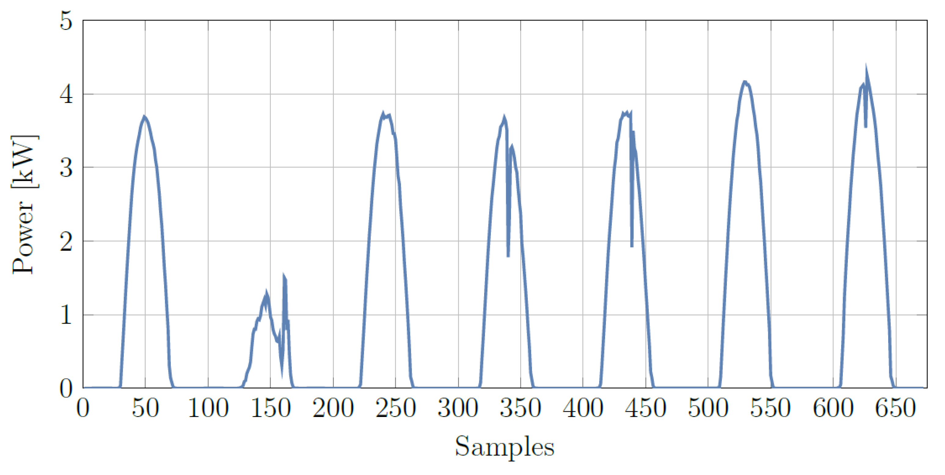
A seasonal analysis is useful to identify any possible meteorological scenario. As will be explained in the following sections, there is a strong association between solar irradiation and PV produced power; as a consequence, the shape of daily generated power can be considered an indicator of the variability of solar irradiance during the day. Figure 5, Figure 6, Figure 7 and Figure 8 show the trends of produced power referred to a single week of each season. It can be noticed that summer and winter are mainly characterized by quite regular days that reproduce a well recognizable shape. In spring and autumn, instead, a significant irregularity occurs that does not allow to identify a typical trend. In

Table 1. PV plant data referred to seasonal periods shown from Figure 5, Figure 6, Figure 7 and Figure 8.

Season	${\mathit{P}}_{\mathit{max}}$ (W)	${\mathit{P}}_{\mathit{mean}}$ (W)	${\mathit{G}}_{\mathit{max}}$ (W/m${}^2$)	${\mathit{T}}_{\mathit{max}}$ (${}^{\circ }$C)
Spring	4912.4	872.4	1237.0	21.7
Summer	3401.8	1101.7	992.5	35.1
Autumn	3538.4	259.5	578.6	18.6
Winter	4256.2	956.9	715.6	16.0

, $P_{max}$, $P_{mean},$$G_{max}$ and $T_{max}$ refer to the maximum and mean PV output power, global horizontal irradiance and maximum air ambient temperature, respectively. It is evident that the higher value of power, and, hence, of irradiance, is encountered in spring; nonetheless, the mean value of power is higher in summer than in spring: this is due to irradiance inconstancy during spring. The lower value of maximum power encountered in summer instead of in spring is due to the increase in temperature that increases the thermal losses and reduces the PV systems output. These facts suggest that a seasonal distinction of data can be useful for the learning process of the network.

In this way, as will be shown, the presented network will be able to forecast power even when dealing with weather irregularities, as a result of an accurate tuning of network parameters based on the analysis of input data.

3.2. Data Pre-Processing

Meteorological parameters have a deep impact on PV power generation. These parameters can differ from one geographical location to another.

Weather parameters and PV power output may experience different correlations, i.e., degree of association with each other, at different locations. The accuracy of a model in the prediction of a certain quantity is linked to the correlation of input and output values of the model itself.

Two methods are presented in literature for estimating the correlation between two variables. The Pearson correlation coefficient is typically used to evaluate the linear relationship between these variables, while the Spearman correlation analysis evaluates the relationship between two variables that change together not necessarily in a proportional manner.

For our purpose, Pearson’s correlation coefficients have been chosen since they are preferred in the case of raw data and for a better reproducibility of the work (most works are based on Pearson analysis); Pearson’s coefficients allow to measure the level of association between two continuous variables and they are based on the method of covariance. The Pearson coefficient, $r_{x,y}$, between two variables x and y is expressed as:

$$\begin{array}{c}\hfill r_{x,y}={\displaystyle \frac{{\sum }_{i=1}^n(x_i-\overline{x})(y_i-\overline{y})}{\sqrt{{\sum }_{i=1}^n{(x_i-\overline{x})}^2}\sqrt{{\sum }_{i=1}^n{(x_i-\overline{x})}^2}}}\end{array}$$

(1)

where, n is sample size, $x_i$ and $y_i$ are the individual sample points indexed with i and $\overline{x}={\displaystyle \frac{1}{n}}{\sum }_{i=1}^n{x}_i$ is the sample mean, similarly for $\overline{y}$.

Pearson’s analysis gives information not only on the magnitude of association, but also on its direction. The Pearson’s coefficient, $r_{x,y}$, can range from −1 to +1 where an absolute value below 0.5 indicates poor association and a value close to 1 corresponds to strong correlation.

Time series data of PV power output and its corresponding weather variables are needed to set up the prediction model. The target of the presented ANN is the DC photovoltaic power forecasted for the next day. Literature reviews [40] report a strong correlation between solar irradiance and PV power output, especially in the case of sunny days, but also when dealing with cloudy or rainy days. These facts are confirmed by our statistical analyses, reported in Figure 9. The relationships existing among available weather parameters, i.e., irradiance, temperature and air humidity, and the predicted quantity are reported in Figure 10 where the analysis has been performed in a time frame of 33 days.

In addition, a time variable is included as input. It is necessary to anticipate some characteristics of the developed ANN that will be better analysed in the following paragraphs. The proposed ANN is supposed to provide a daily prevision of the DC power requirement but, since its training set is constituted by information concerning a set of days before the forecast, a time indication is needed. Data reporting the indication of the month are unnecessary for the network since a constant quantity shows no correlation with a vector, the DC power in our specific case. Moreover, vectors of day, hour, minutes and, eventually, seconds are discontinuous and should not be used when training networks since such discontinuities may lead the learning process to diverge. Hence, a time vector has been considered providing a sinusoidal mapping of the day with time step of 1 min; this allowed to include a continuous representation of the daytime.

While other variables could be considered as input vectors, the increased size of the input matrix will enhance complexity and computational cost of the ANN; as a matter of facts, a central point is the design of a neural model characterized by an optimal size of the input data. This aspect will be discussed in Section 4 where some comparisons are shown between our network and other ANNs making use of a training set comprising multiple variables.

4. Methodology

The literature review of Section 2 stresses the wide use of ANNs in prediction applications thanks to their adaptability and generalization capabilities, including the forecasting of PV produced power.

The well-known Feed Forward Neural Network approximates a mapping function from input variables to output variables and readily learns linear and nonlinear relationships. Owing to its simple architecture, it is capable to achieve good performances with low computational costs. These features also make it widely used in time series forecasting. While feed forward neural networks show great capabilities, the forecasting performances could be improved by using recurrence or reusing past inputs and outputs. A network which remembers previous inputs or feedbacks previous outputs may have greater success in determining time dependent patterns. So, the modified version of the Feed Forward architecture characterized by a dynamic feedback is analysed. Thus, every hidden layer neuron has the ability to process previous values together with new input signals. In this way, the neural network can also learn the temporal dependence that varies with circumstances, in our case with meteorological conditions.

The proposed method is implemented in MATLAB environment that allowed to program our network through a powerful and performing tool; thanks to the Neural Network Toolbox the designing phase is simplyfied allowing the programmer to focus on the most relevant aspects of the ANN implementation, i.e., the choice of the most suitable characteristics (architecture of the network, number of layers and neurons and selection of the most suitable training algorithm) and the analysis and refinement of the data to be used in the training phase.

4.1. Artificial Neural Network Model

A generic ANN architecture consists of input, hidden and output layers that are composed by a set of artificial neurons connected to each other through adjustable connection weights.

The neural unit, shown in Figure 11, can be mathematically expressed as:

$$u_k=\sum _{j=1}^m{w}_{kj}{x}_j$$

(2)

$$y_k=\phi (u_k+b_k)$$

(3)

where $x_j$ are the inputs of a generic neuron k that are multiplied by their respective connection weights, $w_{kj}$ and then summed. The sum is applied to the activation function $\phi$ along with the bias $b_k$ that can be positive or negative, so it can increase or decrease the net input of the activation function.

The ANN ability to provide a reasonable solution can be achieved by means of a training process that consists in iteratively tuning the values of synaptic weights in order to minimize an error defined as the difference between model predictions and real observations. During the training process, the derivatives of the error are back propagated to each layer in order to modify parameters.

One of the most used learning algorithms is the Levenberg-Marquardt that updates weights as follows:

$$w_{k+1}=w_k-{(J_k^T{J}_k+\mu I)}^{-1}{J}_k{e}_k$$

(4)

the error $e_k$ is the difference between the desired and the actual output and J is the Jacobian matrix of the error vector, $e_k$. The parameter $\mu$ is increased or decreased at each step. This cycle continues until the desired output or a stopping criteria, that can be a threshold error or maximum number of epochs, is reached.

A good training is performed if generalization occurs, meaning that the ANN is able to provide a sufficiently accurate result also in response to inputs that are not faced during the training process. If the aforementioned features are achieved, the ANN will be robust also against noisy data.

Usually, the main problem to be addressed is how to choose the number of delays and neurons in each layer. Since there is no exact procedure to solve this problem, the architecture of the ANN is selected on the basis of a trial and error process. As far as the time delay is concerned, it is often necessary, especially when data show a strong time dependence. The setup of a delay needs a detailed stability analysis, because it could cause fluctuation and uncertainties of the ANN; therefore, it is fundamental for the network to reach the global stability at an equilibrium condition. Another important parameter influencing the ANN capabilities is the number of neurons. The optimal number of neurons is chosen by means of a minimum error criteria-based analysis.

As the design of ANN follows a trial and error process in order to select its optimal parameters, several proves need to be made before the final architecture is achieved.

The accuracy measurement of any PV power forecasting model is performed by means of standardized performance errors, such as Mean Square Error (MSE), Root Mean Square Error (RMSE), Mean Absolute Error (MAE), Mean Absolute Percentage Error (MAPE), Weighted Mean Absolute Percentage Error mean (WMAPE), Relative Error (MRE), and Mean Bias Error (MBE) [41].

In our analysis the RMSE and WMAPE are evaluated in order to make an easy comparison with other neural models present in literature:

$$RMSE=\sqrt{{\displaystyle \frac{1}{N}}\sum _{i=1}^N{(y_{forecasted}-y_{target})}^2}$$

(5)

$$WMAPE={\displaystyle \frac{1}{N}}{\displaystyle \frac{{\sum }_{i=1}^N|y_{forecasted}-y_{target}|}{{\sum }_{i=1}^N\left|y_{target}\right|}}\times 100$$

(6)

where n is the sample size, $y_{forecasted}$ are the expected values and $y_{target}$ are the known values.

4.2. ANN Model Development

In our study, to design the best ANN architecture three different conditions are surveyed: these are the variation of the number of neurons, the size of the training set and the difference among a static and a dynamic architecture. The investigation of the most suitable inputs for the ANN training is deeply explained in Section 3. By referring to the correlation analysis, further studies are conducted to select the best combination of available data and the correct size of training set. Hence, to develop an accurate model the following cases of study are analysed:

• Case #1. Selection of appropriate network inputs based on the previous correlation analysis and assessment of the right size of the training set.
• Case #2. After assembling the training set, the ANN capabilities are evaluated by varying the number of neurons.
• Case #3. The performances of an ANN static model are compared with the ones of a dynamic model. We introduce a “memory effect” to the Feed-Forward (static) architecture, providing the network with a dynamic behaviour. As will be shown in Section 4.2.3, the idea is that of supplying the ANN with the last PV power prediction value in order to compose a sort of power time-sequence. In this way, it is possible to exploit the pros of dynamic ANN without implementing a real one, hence avoiding the cons related to them, e.g., need of large computational resources and more complex training processes.

Performances of the ANN are evaluated on the power profiles of Figure 12, each belonging to the last day of the respective season shown from Figure 5, Figure 6, Figure 7 and Figure 8.

4.2.1. Case #1

By referring to the correlation analysis of Section 3, different combinations of inputs are tested and the RMSE and WMAPE of each combination are evaluated. For this analysis, an FF architecture is chosen, the number of hidden neurons is fixed to 10 and the number of days composing the training set is fixed to 20, considered a good trade-off between the size of training set and the complexity of the ANN. Four input combinations are analysed: in each of them time and irradiance vectors are included since the first is fundamental to distinguish days, the second is the most correlated input with the ANN output. Therefore, a first inputs combination, composed by only time and irradiance vectors is considered. The WMAPE obtained is about 37.5%. In the second and third combinations further inputs are added, temperature and air humidity, respectively. Experimental results confirm the levels of association determined by Pearson correlation analyses, reported in Figure 9. The last combination includes all variables. The last three datasets improve the performances but, the second set is the only bringing WMAPE below 15%. The errors obtained for each combination are reported in

Table 2. Weighted Mean Absolute Percentage Error mean (WMAPE) and Root Mean Square Error (RMSE) for different inputs combinations.

ANN INPUTS	RMSE (W)	WMAPE (%)
Time + Irradiance	390.12	37.50
Time + Irradiance + Temperature	120.50	14.97
Time + Irradiance + Humidity	240.78	21.02
Time + Irradiance + Temperature + Humidity	230.66	19.46

. In particular, WMAPE and RMSE are evaluated for each day in Figure 12 and an average of the errors is computed and reported in Table 2.

This analysis allows to select time, irradiance and temperature vectors as the most appropriate ANN inputs.

The second step consists in finding the correct training set size or rather choosing what is the right number of days that need to be included in the training set. In particular, the number of days is supposed to vary in a range from 5 to 30.

Figure 13 shows the WMAPE for each season. It is worth to note that the WMAPE reaches its minimum at 5 days training for summer and winter; as far as spring and autumn is concerned, a set composed by 30 days is necessary because of the variability of weather conditions. Therefore, the size of the training set can be reduced in summer and winter. Definitively the size of the training set in summer and winter consists of 3 inputs vectors, each of 480 samples, while in spring and autumn each input vector is composed by 2880 samples.

4.2.2. Case #2

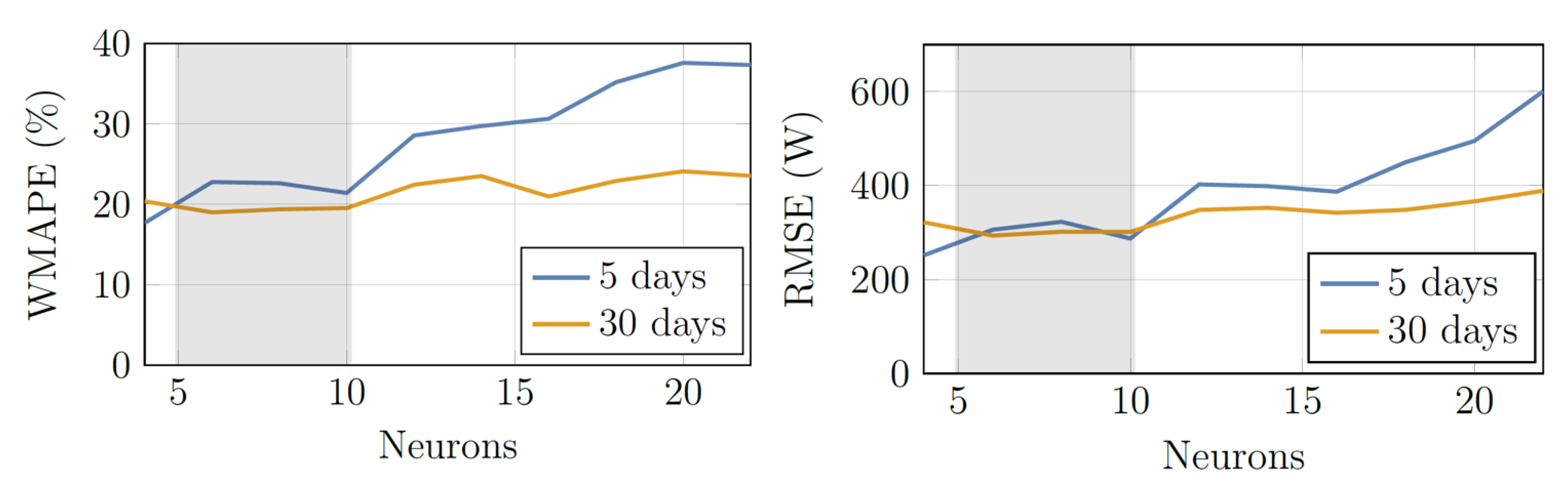
After selecting the most appropriate training set, a further step is necessary, that is to choose the number of neurons in the hidden layer. Several trials have been conducted by varying the neurons from 4 to 22. The results are obtained by considering a training set composed by both 5 and 30 days. Average WMAPE and RMSE errors obtained for each season are evaluated and reported in Figure 14.

It is evident that a training set constituted by 30 days allows to reach a lower error for almost all cases. Furthermore, the errors are similar in a range from 5 to 10 neurons, as shown in Figure 14. Therefore, this work proposes an automatic strategy able to evaluate the best ANN performance, where the ANN inputs are fixed while the size of training set is chosen according to the season between 5 or 30 days and finally the number of neurons varies from 5 to 10. This reconfigurable procedure allows to obtain the best architecture according to the season.

4.2.3. Case #3

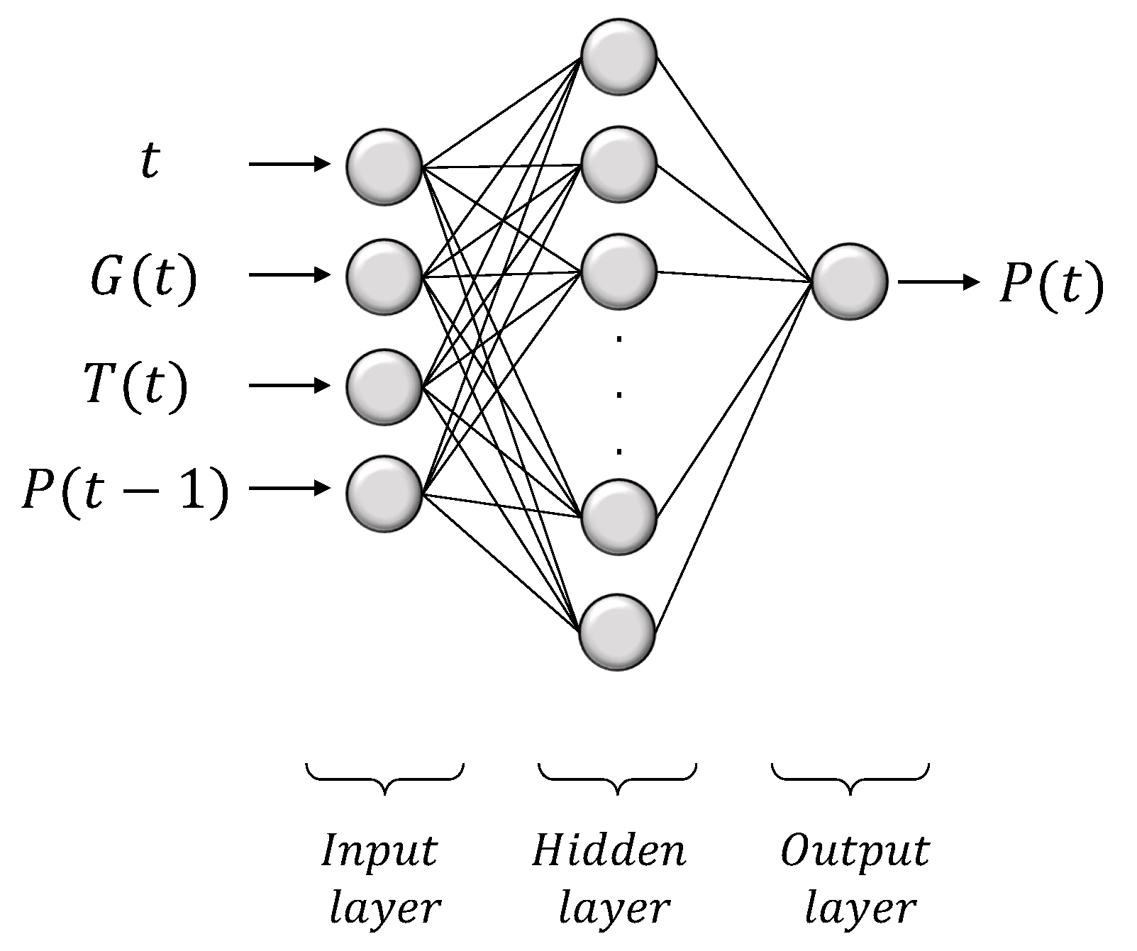
Despite the degree of freedom introduced by the arbitrary choice of the number of neurons, the ANN architecture obtained so far shows good results for sunny days but, in the case of partly cloudy ones the ANN is not always able to achieve generalization. Therefore, a time delay, $\Delta t$, equal to 15 min in the FF architecture is introduced, providing the network with a dynamic behaviour, Figure 15: the DC produced power at time step $(t-\Delta t)$, P(t−$\Delta t$), is included as fourth input.

Table 3. WMAPE and RMSE achieved by static and dynamic neural networkNN.

	WMAPE (%) FFNN	WMAPE (%) D-FFNN
Spring	20.07	14.78
Summer	4.04	3.12
Autumn	21.85	15.63
Winter	6.89	4.21

shows that WMAPE is greatly reduced if a further input is considered. In particular, for summer and winter, it slightly decreases when a D-FFNN architecture is considered. As regards autumn and spring, a significant gain occurs: the error is reduced below the 20%.

An evaluation of the errors concerning the training and validation phases leads to choose a static or a dynamic ANN having a number of neurons varying from 5 to 10 according to the particular day. A summary of the optimal dynamic ANN architecture is given in

Table 4. Summary of dynamic Artificial Neural Network (ANN) parameters.

ANN Parameters
Inputs	3-Time, Irradiance,
	Temperature
Outputs	1-PV power
Number of layers	3-Input, Hidden, Output
Number of hidden neurons	5:10
Number of delay	1-PV power
Functions	Log-sigmoid, Linear
Learning algorithm	Levemberg-Marquardt

.

5. Validation and Results

After the training process, the ANN performances are evaluated by checking if the ANN is able to forecast the power produced in days outside the training dataset; the test is performed over a single day (96 samples for 4 inputs). In particular, three different classes of days have been identified: completely sunny or completely cloudy days, characterized by a regular irradiance shape, quite irregular days that show some spikes coming from few passing clouds and, finally, heavily irregular days in which the original “bell shape” of the PV power production is poorly recognizable. Three different days are chosen, one for each class, that are not part of the training database. This choice allows to test the generalization capabilities of the neural system by considering different scenarios. Figure 16, Figure 17 and Figure 18 demonstrate that the ANN is able to predict PV power with high accuracy for days with different levels of cloudiness. 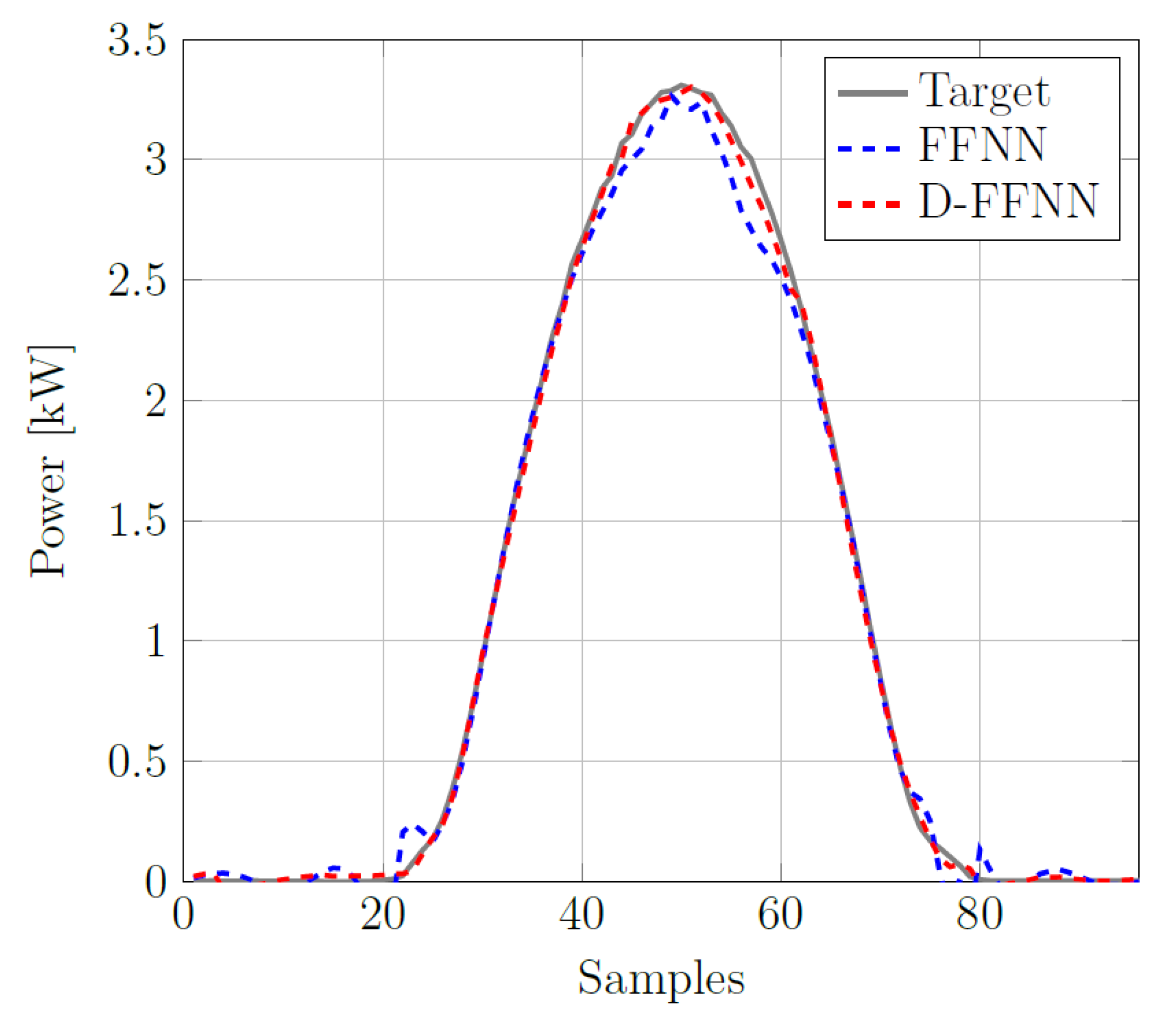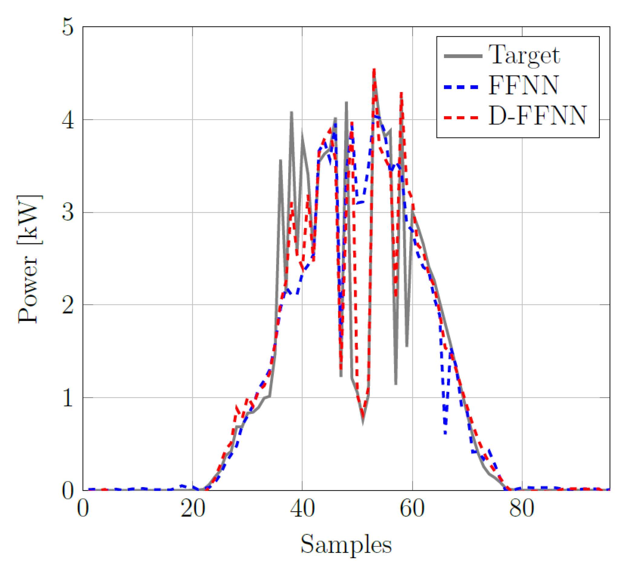In Figure 16, Figure 17 and Figure 18 the continuous line represents real measurements while the discontinuous blue and red lines refer to the FFNN and D-FFNN predictions, respectively.

Figure 16 illustrates the prediction of both ANN types for the 7 July 2019, an example of sunny day with few weather variations. The FFNN architecture including 6 neurons allows to get a WMAPE around 3.7% and a RMSE of 39.8; on the other hand the D-FFNN architecture with 5 hidden neurons reaches a WMAPE equal to 2.64% and an RMSE of 34.98.

Figure 17 is referred to the 10 January 2019, classifiable as a quite regular day with a small amount of cloudiness. The FFNN architecture including 8 neurons achieves a WMAPE around 17.62% and a RMSE of 289.8; on the other hand the D-FFNN architecture only takes 5 hidden neurons to obtain a WMAPE equal to 11.41% and RMSE of 206.03.

Finally, Figure 18 shows the prediction obtained for the 4 April 2019, a strongly irregular day characterized by a high level of cloudiness: the WMAPE is 28.41% and 21.11% for FFNN and D-FFNN, respectively, while their respective RMSE are about 701.02 and 540.75. In this case, the FFNN and D-FFNN architectures includes 10 and 7 neurons, respectively.

The analysis conducted on these three different days demonstrates that the proposed neural system properly works. Moreover, it is worth noting that a higher degree of cloudiness corresponds to irregular shapes of output PV power, that are responsible for higher errors in the prediction. In order to guarantee an acceptable error, the number of neurons belonging to the hidden layer in the FFNN architecture has to be increased. If this is not enough, our strategy involves the inclusion of a quarter of hour delay that provides a dynamic behaviour to the network and allows to improve the accuracy of the forecast. Indeed, when providing the ANN with a delay, the network turns into a memory-based method, D-FFNN. In this way, its output at any given time is depending on both the present inputs and the history of past outputs. In our case, the introduction of a delay allows to catch any power fluctuation caused by uneven shading conditions in order to take these variations into account in the training phase of the neural network and to improve its performances. Hence, a more complex architecture, D-FFNN, is exploited only for days showing an irregular shape. This adaptability represents the key of our neural system, that is able to daily forecast the power output with great accuracy, also in variable weather conditions. This feature makes the system suitable to be incorporated in smart grids, both for forecasting the generated PV power in a short term and for improving smart energy management.

Lastly, a comparison is reported between the proposed method and other forecasting methods recently presented in the literature. In [42] an RNN-based PV power prediction method is presented. It is possible to compare this approach with our strategy as far as the seasons winter and summer is concerned; as a matter of facts, for such seasons two days are chosen in the cited article whose irradiance profiles can be compared to ours in the case of quite regular irradiance shapes. The reported WMAPE for winter and summer is respectively 6.36% and 1.94%, while our results are 3.12% for summer and 4.21 % for winter; hence the average WMAPEs of the two cases are comparable, but we avoided the use of complex ANN architectures. Another work in which an ANN is used is [43]; in this work an LSTM neural network is used. WMAPE is reported to be among 20% and 48% according to the season in exam, while in our case it is always below 20%. Moreover, in [44] another ANN-based PV power prediction method is shown. In particular, the ANN is trained with satellite images. The paper reports an improved WMAPE of 22.5%, slightly above the values reached by our method. [45] presents an SVM-model for one day-ahead forecasting of PV power for different weather conditions, such as clear-sky, cloudy and rainy days. The forecast ability is expressed by means of MAE that is around 28 and 35 W for regular and irregular weather conditions, respectively; our strategy allowed to reach a MAE of 2.9 and 17.1 W, respectively. Additionally [46] obtains high performances for sunny and partially cloudy days by implementing an MLP-based forecaster. The MAE achieved is below 15 W for all investigated cases, quite similar to the results we reported in

Table 5. Mean Absolute Error (MAE) achieved by the reconfigurable ANN.

	MAE (W) FFNN	MAE (W) D-FFNN
Sunny day	5.3	2.9
Partly cloudy day	31.3	12.0
Variable day	21.65	17.1

.

Hereafter, the results achieved by our neural approach are illustrated. It is evident the increasing complexity in providing an accurate prediction when dealing with shape irregularities of power profile. The MAE achieved by the reconfigurable ANN for three days with increasing levels of irradiance irregularity are reported in Figure 16, Figure 17 and Figure 18, respectively.

Table 5 shows that for regular days both networks achieve a high level of accuracy: the MAE is below 6 W. As already demonstrated by MAPE evaluation for partly cloudy and variable days, the D-FFNN shows better results than FFNN architecture with a MAE below the 20 W. Among the recent methods in literature, the hybrid models allow to reach a lower error, but as mentioned in the literature review, their disadvantage depends on their complexity. Therefore, our reconfigurable model could represent a valid alternative to existing methods thanks to its simplicity and its high performing ability to forecast PV power.

6. Strategy for Energy Flows Management

Apart from the need of simply forecasting the amount of PV power production, the knowledge in advance of such a quantity is of paramount relevance in the protection of the battery bank constituting the storage system of a PV system. The forecasting strategy presented so far is just a piece of a broader method aimed at extending the lifetime of batteries by avoiding stress conditions on the energy storage system. Since it is possible to exchange power between the PV generator, the grid and the storage system, it is necessary to implement a technique for managing such power flows within the EMS (Energy Management System) controller of which the ENEA smart PV system is equipped, Figure 19. The EMS includes the embedded controller of National Instruments CRIO 9068 suitable for controlling and monitoring applications that includes an FPGA and a real-time processor running the NI Linux Real-Time operating system.

The system consists of a computer that allows communication with the instruments and sensors placed on the PV system. As afore mentioned, the implemented strategy constitutes an important tool in the power management of smart grid. With the availability of both PV power production prediction and electrical load consumption estimation, a computation of power surplus or deficit will be done, in order to establish which one will be applied between the energy storage system and the grid. In literature, it is possible to identify two main flux management strategies:

• Standard management for self-consumption. In the time intervals in which the power generated by the photovoltaic panel is greater than that required by the user load, the excess part is supplied to the battery pack, until it reaches full charge. When the storage system can no longer absorb power, this is fed into the grid. Otherwise, when the power supplied by the generator is lower than that required by the load, this is fed by the storage system until it is completely discharged and then by the mains. With this management technique, the storage system is subject to continuous charge and discharge cycles, thus limiting its average life. Furthermore, there is a risk of feeding high power peaks into the network which would worsen the desired quality.
• Peak-shaving. With this technique we try to eliminate the drawbacks of the standard self-consumption technique; as a matter of facts, in this case the excess power is fed into the network and only if this excess is very high is it supplied to the storage system. This ensures a longer average life of the accumulator and limits the power peaks fed into the network, safeguarding the quality of energy. However, not knowing how the trends of the power requested by the user and that supplied by the PV will go, there is a risk of creating a condition in which the accumulator never supplies the load, thus leading to an underuse of the storage equipment and significantly reducing self-consumption, a primary advantage in the installation of photovoltaic systems (or in general of renewable energy systems).

The forecasting method shown in this paper, instead, is a basic block that, combined with an accurate electrical load prediction, has suggested the idea of developing a strategy for an optimal management of batteries charge/discharge. In this context, the idea was born of introducing the potential of forecasting techniques into energy management systems and in particular of energy flows between production plants and storage systems, Figure 20. In particular, if a higher power profile and therefore a large excess of power is expected, the charge of the cells is slowed down, preferring the input into the grid; otherwise, if the excess power is lower, the storage charge is accelerated and then the load can be powered. With this management, an average battery life should be obtained that is considerably longer than in the previous cases, guaranteeing the quality of the network and consumer savings, through a smart management of power flows. To implement this management model it is therefore necessary to dispose of a predictive model for the maximum power profile of the PVs and of the load.

7. Conclusions

An accurate PV power forecasting method has been developped based on a reconfigurable Feed Forward neural network. Definitely:

• A detailed analysis has been carried out, showing the importance of weather conditions and their influence on PV power; as a result of this, the atmospheric variables that have the greatest impact on PV power production have been identified and used as inputs to train the ANN.
• An accurate study of the irregularity of daily irradiance has led to the development of a neural model with great plasticity and capable of reducing the complexity of its architecture when it is not needed. The resulting ANN can be defined tunable since it adapts itself according to the particular irradiance profile.
• After the simulation performed in MATLAB environment, validations have been done for a practical PV plant located in ENEA Casaccia RC (Rome, Italy), using the proposed forecasting neural model.

The ability to reduce the uncertainty of generated power makes the model particularly suitable for integration into smart grids, where the key point is the energy management. The results demonstrate that the achieved accuracy is very high, also under variable weather conditions. This strategy is inserted in a broader scenario where we wish to achieve good results in the optimization of the processes of charge/discharge of the storage system, in order to extend the life-time of the battery pack. A further step will be the developent of an effective method for forecasting the electrical load consumption.